Tests on composite slabs and evaluation of relevant Eurocode 4 provisions

City, University of London Institutional Repository

Citation

:

This is the accepted version of the paper.

This version of the publication may differ from the final published

version.

Permanent repository link: http://openaccess.city.ac.uk/13900/

Link to published version

:

Copyright and reuse:

City Research Online aims to make research

outputs of City, University of London available to a wider audience.

Copyright and Moral Rights remain with the author(s) and/or copyright

holders. URLs from City Research Online may be freely distributed and

linked to.

City Research Online: http://openaccess.city.ac.uk/ [email protected]

1

Tests on composite slabs and evaluation of relevant

Eurocode 4 provisions

Thomas N. Salonikios1, Anastasios G. Sextos2, and Andreas J. Kappos2

1 _{Institute of Engineering Seismology and Earthquake Engineering - EPPO,}

Thessaloniki, Greece

2 _{Civil Engineering Department, Aristotle University of Thessaloniki, Greece}

Abstract. The paper addresses some key issues related to the design of composite slabs with

cold-formed profiled steel sheets. An experimental programme is first presented, involving

six composite slab specimens tested with a view to evaluating Eurocode 4 (EC4) provisions

on testing of composite slabs. In four specimens, the EC4-prescribed 5000 load cycles were

applied using different load ranges resulting from alternative interpretations of the reference

load Wt. Although the rationale of the application of cyclic loading is to induce loss of

chemical bond between the concrete plate and the steel sheet, no such loss was noted in the

tests for either interpretation of the range of load cycles. Using the recorded response of the

specimens the values of factors m and k (related to interface shear transfer in the composite

slab) were determined for the specific steel sheet used in the tests, on the basis of three

alternative interpretations of the related EC4 provisions. The test results confirmed the need

for a more unambiguous description of the m-k test and its interpretation in a future edition of

the Code, as well as for an increase in the load amplitude range to be used in the cyclic

loading tests, to make sure that the intended loss of bond between the concrete slab and the

steel sheet is actually reached. The study also included the development of a special-purpose

software that facilitates design of composite slabs; a parametric investigation of the

2

Keywords: composite slabs, profiled steel sheets, m–k factors, longitudinal shear, load

cycles, Eurocode 4, chemical bond loss, design software.

1. Introduction

The use of cold-formed profiled steel sheets for the construction of composite slabs is an

increasingly popular technique in the construction sector in Europe. A key aspect of the

design of composite slabs according to the pertinent European code, Eurocode 4 (CEN, 2004)

is the determination of factors “m” and “k” used to estimate the longitudinal shear strength of

the composite slab. These factors are unique for each cold-formed profiled steel sheet and

have to be determined experimentally according to the procedure described in Annex B of

EC4. The work reported herein includes the determination of these factors for a specific type

of steel sheet and focuses on the evaluation of EC4 provisions in the light of the measured

response of the test specimens.

Due to its relevance to design, this longitudinal shear test has been carried out in the past

by several researchers. Marimuthu et al. (2007) tested 18 composite slab specimens, the main

test parameter being the shear span. It was found that if the shear ratio is high enough, but not

higher than about 12, the behaviour of the slab is governed by flexure, while for shear ratios

lower than about 4, strength of the slab is governed by shear bond failure. They also found

that by applying the loading cycles prescribed by EC4 the strength of the slab is not reduced

with respect to the strength of the monotonically loaded specimens. The longitudinal shear

resistance of a steel-concrete composite bridge deck was examined by Jeong et al. (2007),

who found that to define the longitudinal shear resistance of such composite decks subjected

to surface loads, it is desirable to use test data with sufficient shear span length, so that the

effect of the normal force at the interface becomes negligible. A simplified method for

estimating the shear strength of composite slabs was proposed by Lopes and Simoes (2008)

3

yields more reliable results than the EC4 method, but note that further experimental

verification is necessary. Calixto et al. (2009) compared the m-k method and the Partial

Connection method (allowed as an alternative by EC4) in the light of experimental results.

Good correlation between the two methods was found, which is not in line with the finding of

Marimuthu et al. (2007) that the two methods provide results differing (on the average) by

26%. Tzaros et al. (2010) tested four composite slab specimens and determined the m and k

factors from the line resulting from linear interpolation between the points defined by the

measured specimen strength, taken as the one corresponding to longitudinal shear failure

(brittle loss of chemical bond between concrete and the steel sheet); they found that the m

-factor is governed by the tensile stress of the steel sheet along the length between the load

point and the middle point of the specimen. The experimental results were well reproduced by

the rather sophisticated analytical model developed by these authors, which is not intended for

design purposes. A similar test programme involving 9 composite slab specimens was carried

out by Tsalkatidis & Avdelas (2010), who used a 3D numerical model set up in a commercial

program (ANSYS), to predict the test results, and found good agreement in terms of load vs.

deflection diagrams.

In the framework of the study presented herein six composite slab specimens were tested.

The main parameters studied were the span (hence the shear ratio), the upper and lower load

level applied during the cyclic loading, and the estimation of m and k factors using alternative

interpretations of the pertinent EC4 provisions. The need for a more rational definition of

some of the parameters prescribed by the Code was made clear by the findings of this study,

and is discussed in Section 5. The paper concludes with a brief presentation of a

special-purpose software developed to facilitate design of composite slabs, which is used for a

4

2. Research Significance

The tests required for the determination of design values for m and k factors are described in

detail in Annex B of EC4. However, some of the code provisions are open to different

interpretations. In paragraph B.3.4(3) the load Wt is defined as the measured failure load of

the preliminary static test. In paragraph B.3.4(5) the same term Wt is defined as the “failure

load”, to be calculated as the maximum load imposed on the slab at failure plus the weight of

the composite slab and spreader beams. Intuitively, the second definition is more rational

since self-weight of the specimen and the load of the spreader beams result in additional

longitudinal shear. For the specimens tested herein, the weight of the spreader beams when

added to the self-weight of the slab gives a force higher than 0.2Wt which is the lower level

applied during the 5000 loading cycles. For this reason two different amplitude levels 0.2Wt

and 0.6Wt were used in the tests, as described in Section 3.

Another point of interest is whether the upper level of cyclic loading (0.6Wt) is sufficient

for inducing loss of bond between concrete and the steel sheet. Since the Eurocodes do not

include a commentary and no relevant background documents were found by the authors, it is

not known whether the intention of the EC4 provisions is to verify that concrete and the steel

sheet can sustain 5000 load cycles without loss of bond, or, on the contrary, the applied cyclic

loading is meant to induce loss of bond and the purpose of the subsequent monotonic loading

test is to estimate the capacity of the composite slab after loss of chemical bond.

A third point open to interpretation is the definition of 'failure load' from the load –

deflection diagram determined from the tests (discussed in Section 5 of the paper). Hence,

three alternative interpretations of the loading to be applied were made in the present

experimental study:

5

 Use of 80% of the aforementioned value whenever the failure load does not exceed by at least 10% the load that corresponds to slip equal to 0.1mm between the steel sheet

and concrete; in this case the response is not considered by EC4 as ductile. In the light

of the relevant literature and the present tests, the authors believe that this case

deserves further consideration.

 Use of the ultimate (post-peak) strength, related to friction mechanisms developing after loss of chemical bond, and manifested by local buckling of the steel sheet.

For comparison purposes, for the tested specimens all three cases were considered, and m and

k values were calculated separately for each case.

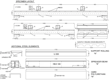
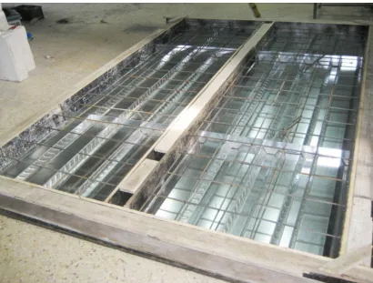
3. Test description

The specimens (Fig. 1) were designed and manufactured (Fig. 2-3) mainly with a view to

determining the m and k factors, which have to be defined through testing for every newly

produced steel sheet, meant to be used in composite slabs, for the design against longitudinal

shear. This check is typically the most critical for the design of composite slabs; hence EC4

describes in detail the entire procedure (in section 9.7.3 and in Annex B, paragraph B.3). The

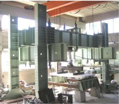
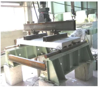
experimental setup with the specimen ready for testing is shown in Figures 4, 5.

The concrete used had a mean compressive (28-day cylinder) strength of 24.7MPa, with a

standard deviation of 1.8MPa, resulting in a characteristic (5% fractile) value of 21.7MPa,

which for all practical purposes can be assigned to EC2 class C20/25. The reinforcement

placed on the upper side of the slab (mainly for shrinkage cracking control) was a single grid

of 8mm bars spaced at 200mm. The nominal yield stress of this reinforcement was 500MPa

and the maximum available strain (εsu) was greater than 7.5%. The proprietary steel sheet

used in the composite slab was 0.75mm thick; its cross section is shown in figure 1

6

strain Fig. 6. Six specimens, in two groups of three, were manufactured; each group was

characterised by the length (hence the shear span) of the specimen. The span was 3.20m for

group CPLL (Fig. 4) and 2.00m for group CPLS (Fig. 5); the corresponding shear spans are

10.6 and 4.2. Crack inducers were placed at the loading point of all specimens, as prescribed

in section B3.3 of EN1994-1-1 (CEN, 2004). One specimen in each group was loaded (with

displacement control) monotonically to failure. The other two specimens were subjected to

5000 load-controlled cycles within predefined limits 0.2Wt and 0.6Wt, where Wt is the failure

load measured during the test of the first specimen. These specimens were then subjected to

displacement-controlled loading to failure. It is pointed out that if Wt is defined as the total

ultimate load of the slab (i.e. including the weight of the composite slab and spreader beams,

see B.3.4 of EC4), then the 0.6Wt limit is clearly defined. However, in this case there is a

issue with the definition of the lower limit 0.2Wt, since this load was found to be less than the

weight of the slab and the spreader beams used, hence a tensile force would be needed to

materialise this lower limit, which is unrealistic and most probably is not the actual intention

of the Code. Since the authors did not find any justification notes regarding this particular

clause of EC4, the following loading programme was finally implemented: One specimen was

subjected to 5000 load cycles with an upper limit of 0.6Wt as defined previously (total

strength of the specimen plus the self weight of the spreader beams and the slab), and a lower

limit of 1/3 the net load (i.e. the load applied through the hydraulic jack) of the upper limit,

hence maintaining the max/min ratio envisaged by the Code for the net forces only. Using this

interpretation the 5000 cycles applied to specimen CPLL2 corresponded to an upper limit of

9kN and a lower limit of 3kN; taking into account the self-weight and the weight of spreader

beams (14.95kN) the corresponding total loads Wt were 23.95kN and 17.95kN, respectively.

During this test no loss of chemical bond between the steel sheet and the concrete slab was

7

conservative, interpretation, increasing the load limits for specimens CPLL3, CPLS2 and

CPLS3. The applied load cycles now had limits 0.2Pult and 0.6Pult where Pult was the

measured ('net') failure load recorded during the test of specimens CPLL1 and CPLS1. This

way, the applied loads varied between 4kN and 12kN for specimen CPLL3, with

corresponding total loads 18.95kN to 26.95kN when self-weights are taken into account. The

value 20kN is the failure load that was recorded during the test of specimen CPLL1. During

the test of specimen CPLS1 the recorded failure load was 42.33kN, with self weight 10.63kN.

The applied loads varied from 8.46kN to 25.40kN for specimens CPLS2 and CPLS3 (total

values from 19.09kN to 36.03kN). It was found that although the applied loads (5000 cycles)

were increased, no loss of chemical bond at the interface between the steel sheets and the

concrete topping was detected in the specimens. Chemical bond was lost when the specimens

were loaded monotonically, subsequent to the cyclic loading sequence.

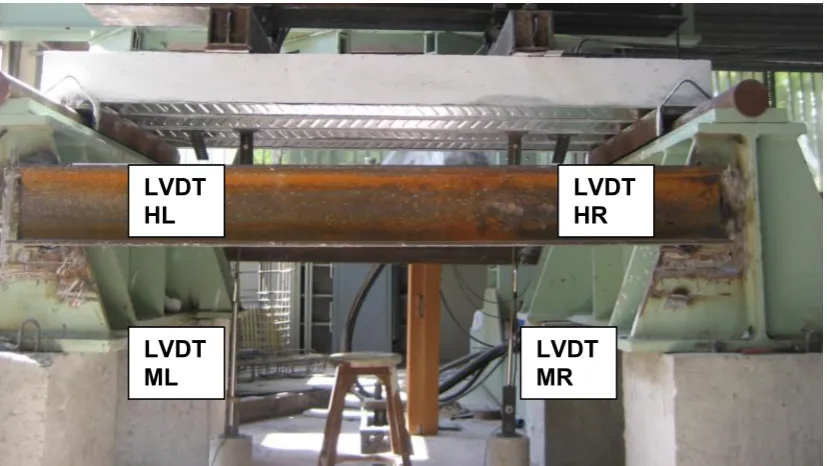
The composite slabs were instrumented with four displacement transducers (LVDTs),

whose layout is shown in Fig. 7. These were used to measure the deflection in the span of the

specimen at the loading points, Middle Left (ML) - Middle Right (MR), and another two

transducers, Horizontal Left (HL), Horizontal Right (HR), were used to measure the sliding of

the steel sheet relative to the concrete topping at the lower face of the specimen. The diagrams

given in the next section plot the displacement measured by these LVDTs and are named as

δML, δMR, δHL, δRL respectively. The data “Ptot” plotted on the vertical axis is the total load

recorded during the tests, that includes the load of spreader beams and the self weight of the

specimens.

4. Specimen Response and Test Results

Figure 8 illustrates the specimen CPLL1 during the test. The crack at the left loading point is

also shown enlarged in the same figure. Figure 9 depicts the slip between the steel sheet and

8

“HL” is shown. This specimen was loaded by monotonically increasing imposed

displacements. It is noted that while there is significant capacity of the concrete topping in

compression and of the steel sheet in tension, the parameter defining the resistance of the

composite slab is the transfer mechanism between these two materials. Prior to debonding the

interface shear stresses are resisted primarily by chemical bond. During the test of specimen

CPLL1, for a deflection between 2 and 3mm, the chemical bond between the steel sheet and

the concrete topping was lost and a flexural crack formed under the left loading point (Fig. 8).

At this point the strength of the specimen was reduced by about 50% and the deflection at the

left loading point was increased to 5mm. As the imposed displacement was increased the

strength of the specimen started to pick up again but with significantly lower stiffness. While

prior to debonding the steel sheet acted as tension reinforcement, the load resisting

mechanism activated after loss of bond included the flexural strength of the (bare) steel sheet

and friction between concrete and the steel sheet, more specifically mechanical interlock at

the embossments and friction at the remaining surface of the sheet. It must be noted that the

flexural strength of the steel sheet is increased, due to the presence of concrete at its top,

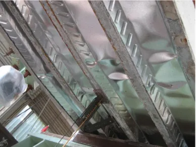
which offers restraint against local buckling phenomena in the steel sheet; such buckling

appeared (Fig. 10) for a higher imposed displacement than that which would appear if the

sheet was loaded as an (unrestraint) simply-supported beam. The post-debonding mechanism

proved to be quite effective and the strength of the specimen picked up, reaching maximum

values at imposed displacements between 20 and 25mm (Fig. 11), which are about 10 times

those at debonding.

Despite the nominal symmetry of the test set-up, only in two specimens the main flexural

cracks formed at both loading points; in all others only one major crack formed, either on the

left or on the right side, and most of the inelastic deformation concentrated therein. For some

9

crack formed. For high inelastic deformations local buckling occurred at the compression side

of the steel sheet, under the points of flexural cracks in concrete (Fig. 10).

In Figures 11 and 12, load – deflection curves are shown for the high (10.6) and low (4.2)

shear ratio specimens, respectively; each diagram is plotted for the side of the specimen where

failure occurred. It is clear from the diagrams that the resistance due to friction mechanisms

(reached at deflections of 20 – 25mm) is only about 10% lower than that prior to debonding in

the CPLL group, and almost the same in the CPLS group. It is noted again that the maximum

resistance is reached at only 2 to 3mm of deflection, which clearly shows the importance of

the post-debonding mechanism to the deformability of the composite slab. The post-peak

branch of the load-deflection curve is favourably affected by the ductile stress–strain diagram

of the steel sheets (Fig. 6).

Slip between the steel sheet and concrete was measured at both ends of the specimens and,

as expected was higher at the end where the main crack formed. The measured slip

displacements are about 15mm at the end of the test, as shown in the load vs. longitudinal slip

diagrams of Figures 13 and 14. It is pointed out that debonding occurred in both the low and

high shear ratio specimens, the only difference being the deflection at which debonding took

place, which was higher in the CPLL group (high shear ratio).

5. Estimation of m and k factors using alternative approaches

The shear forces measured in the tests were used for the determination of m and k factors,

needed for the verification of the composite slab against longitudinal shear; these shear forces

(Vt) are equal to half the values of the developed strengths and are shown in Figures 11 to 14.

From the tests of two groupsof composite slabs, each of which included three specimens, the

variation in measured strength did not exceed 10% in each group. Therefore, according to

10

10%. The line plotting the normalised Vt vs. Ap values was then drawn, from which m=82.23,

k=0.028 was found.

A critical point mentioned in paragraph B.3.5(1) of EC4 is discussed in the following. This

paragraph states that if the behaviour is ductile, the representative experimental shear force Vt

should be taken as 0.5 times the value of the failure load Wt as defined in B.3.4. If the

behaviour is brittle this value shall be reduced by a factor 0.8. According to paragraph

9.7.3(3) the longitudinal shear behaviour may be consider as ductile if the failure load exceeds

the load causing a recorded end slip of 0.1mm by more than 10%. As can be seen in the load

vs. horizontal slip diagrams, given in Figures 13 and 14, the measured slip is 0.1mm at the

beginning of the first descending branch of the diagram. It has to be stressed that this rule is

defined on the basis of values that are very sensitive to estimate from the test results and have

no clear physical meaning. In contrast, there is physical meaning in the comparison between

the minimum strength (strength reduction after loss of chemical bond between the steel sheet

and concrete topping) and the strength that is developed between steel and concrete through

the friction mechanism. This indicates that subsequent to loss of chemical bond, a stable

system results with significant strength, very close to the strength at the loss of chemical

bond, as noted in the previous section. According to this, the response that is shown in

diagrams 11 and 12 is considered ductile and the values that were calculated above, m=82.2

and k=0.028 are valid. If the factors m and k are calculated according to the 'unfavourable'

interpretation of EC4 (reduction of 0.9Wt by 20%), the resulting values are m=66.08, k=0.022.

Finally, another approach for estimating m, k was applied. According to this, the factors m

and k are calculated on the basis of the shear force resisted by the friction mechanism (i.e. not

by the shear force at the point of loss of chemical bond, prior to the first strength drop). As

mentioned previously, the strength due to chemical bond and the strength due to friction

11

the resulting line has a steeper slope than in the other two methods, m=91.04, but smaller

initial ordinate, k=0.0117. The diagrams that show the lines that define the m and k values for

each case are given in Fig. 15, both separately and in a comparative diagram.

6. Software for the Design of Composite Slabs

As part of the present study, special-purpose software for the design of composite slabs with

profiled steel sheets was developed, based on Eurocode provisions and engineering judgement

where appropriate. VB.NET programming language was used in a windows-based,

user-friendly, stand alone application.

This section focuses on the software’s capability to perform parametric evaluation of shear

strength for a set of structural configurations (i.e., number of spans, span lengths, loading, and

boundary conditions). The key requirements were to: (a) facilitate the investigation of the

impact of different approaches for the estimation of m-k factors on the overall design of

composite slabs, (b) fully comply with the current code framework (i.e., Eurocodes 2, 3 and

4), (c) assist the designer to use typical sheet profiles in practical applications, while acquiring

a deeper understanding regarding the mechanics of the behaviour of the profiled sheet through

a transparent computational scheme where all assumptions and calculations are made

available at every step, and (d) evaluate the effectives of design separately, for the

construction stage and the operation stage.

The program flow is straightforward and no prerequisites are needed. At start-up, the

designer can first input the general information related to the project under study and decide

the basic parameters of the problem. This is actually the only action initially available, in the

sense that other options are not yet accessible but “unlock” gradually to establish a clear,

“one-way flow”. Next, the (geometrical and material) section properties of the profiled sheet

are given by the user, followed by the definition of the desired composite slab section and the

12

moments, negative bending moments, vertical shear and longitudinal shear forces (Figure 16).

At the same time, all calculations made are recorded on a separate logfile to provide a

transparent overview of the analysis steps and facilitate an in-depth understanding of the

design process. Having defined the desirable profiled sheet and composite slab section, the

designer can specify the structural system of the slab. A continuous beam of up to 10 spans

can be described (Figure 17). The beam is solved with the use of the three moments

(Clapeyron) method. There is no limit as to the length (L) of each span or to the live load (Q)

set, while the self weight (G) of the steel sheets (required for the construction phase) and of

the composite slab (for the operation phase) are calculated automatically. The structure is

solved for the load combination G + Q for the construction phase and for 1.35G +1.50 Q for

the operation phase; however, the user can choose independently the critical distribution of

the live load among the various spans. The software also permits consideration of different

support conditions, as well as the existence of cantilevers at either end of the beam. In this

way, the vast majority of the structural systems used in practice can be tackled. Note that, as

before, all input data and analysis results are monitored and recorded in the logfile which

appears on the right hand column of the program, while the user can visualize the calculated

bending moments and shear forces to be developed during the construction and operation

phases (Figure 17). The deformed shape of the slab can also be determined. Finally, it is the

designer’s decision to modify the length of the spans or the value and distribution of the live

loads to investigate the critical cases where the resulting action effects (bending moments,

shear forces, and deflections) exceed the computed allowable resistance or deformation limits.

Design verifications for the ultimate and serviceability limit states are performed by the

software (Figure 18) right after completing structural analysis. The checks are conducted for

all spans of the structural system, given the fact that both the resistance to longitudinal shear

13

By visualizing the developed capacity-to-demand ratio, in the form of safety factors,

referring to flexural resistance, shear resistance, and deformations of the system, the user can

re-design the system using his/her engineering judgment, either by providing a stronger sheet

or thicker slab sections or by changing the structural system by introducing intermediate

(temporary) supports. Moreover, the impact of different m-k values on the overall design

process can be parametrically studied, as described in the following section.

7. Impact of m, k factors on the shear strength of the composite slab and the

corresponding failure mode

Using the developed software and the experimentally defined values of the m, k factors, sets

of design tables can be prepared, such as Tables 1 and 2, for different combinations of slab

thickness, span length and structural system (different number of spans). The critical live load

q in each case is determined based on the specific prevailing mode of failure (i.e. flexure

under positive and negative bending, longitudinal shear, and vertical shear); note that the

tables do not include values q<1kN/m2_{, as these are not relevant for design. Such tables are}

useful for a quick selection of the composite slab configuration in practical applications.

Moreover, an effort was made to investigate the effect of determining the m-k values on

the basis of alternative assumptions, as discussed in Section 5. Some selected results are

shown in Tables 3 and 4, which refer to the most critical case of a thick (200mm) slab. Also

shown (to the right of the main tables) are the calculated values of shear resistance, both

transverse (VvRd) and longitudinal (VLRd). For the first two sets of m-k, it is seen that in most

cases (typically for span length L<3.0m) the effect of different m-k determination is generally

low as differences in the allowable live load do not exceed 10%. On the contrary, it becomes

significant (at least in terms of percentage change) in case of long spans (L>3.0m). It has to

14

kN/m2) and such a solution would not be acceptable in most practical applications. It was also

observed that when the span is short (i.e., L=1.0), the prevailing mode of failure is ‘vertical’

shear, hence the alternative definition of the m-k values does not affect the design. However,

in all other cases (L>1.25m, or shear ratio αs≥7.8) longitudinal shear governs the final design.

For all these cases, the assumption regarding strength after loss of chemical bond leads to

only a marginal increase in the maximum permissible live load. This can be attributed to the

fact that, in contrast to other modes of failure, the longitudinal shear strength is a function of

the span length. The use of the conservative estimate of m-k (66.08, 0.02) leads to

significantly lower levels of maximum permissible live load due to its inferior (by

approximately 20%) resistance to longitudinal shear. It is also noted that this effect becomes

more significant for longer span lengths, independently of the number of spans.

8. Conclusions

In the light of the present experimental work, EC4 provisions related to longitudinal shear in

composite slabs were critically assessed, focussing on the definition of: (a) the upper and

lower limit of the applied 5000 load cycles, and (b) the failure load that should be considered

in the determination of m and k factors. It was concluded that the limits 0.2Wt and 0.6Wt

should be defined in a more pragmatic and unambiguous way, making sure that the load to be

applied through the hydraulic jack is always realistic. Although the second interpretation of

the cyclic load limits proposed herein (based on the measured 'net' failure load recorded

during the monotonic test of the specimen) is more conservative, no loss of chemical bond

during the application of 5000 cycles was observed. It is concluded, therefore, that factors 0.2

15

For the estimation of m and k factors the strength that should be taken into account should

also be defined appropriately. In the framework of the present study three interpretations of

the EC4 provisions were explored:

 Use of the load corresponding to maximum strength, developed just prior to loss of chemical bond.

 Use of 80% of the aforementioned value whenever the failure load does not exceed by at least 10% the load that corresponds to longitudinal slip equal to 0.1mm.

 Use of the ultimate (post-peak) strength, related to friction mechanisms developing after loss of chemical bond, and manifested by local buckling of the steel sheet.

The second interpretation is the more conservative one, and the resulting m-k factors are

lower. The third interpretation results in lower k factor and higher m factors than in the first

interpretation.

To further demonstrate the implications of the above issues on the design process, an

analytical approach implemented into a computer software was developed, based on Eurocode

provisions and engineering judgment. It was found that the method of predicting the m-k

factors has a visible influence on the design of composite slabs, since for medium and high

values of the shear ratio, longitudinal shear governs the final design. It is therefore clear that

this important point of EC4, related to the reliable estimate of longitudinal shear resistance,

should be clarified in a future edition or amendment of the Code.

Acknowledgement

The research project, results of which are present in this paper, was funded by Panelco S.A.,

Greece (http://www.panelco.gr/ ). The support of Dr K. Antoniades (from Panelco) during all

16 References

Calixto, J.M., Brendolan, G. and Pimenta, R. (2009), “Comparative study of longitudinal shear design

criteria for composite slabs”, Ibracon Structures and Materials Journal, 2(2), 124 – 141.

CEN [Comité Européen de Normalisation] (2004), Eurocode 4: Design of composite steel and

concrete structures. Part 1-1: General rules and rules for buildings, EN 1994–1–1, Brussels.

Jeong, Y.J., Kim, H.Y., Koo, H.B. and Park, S.K. (2007), “Longitudinal shear resistance of

steel-concrete composite bridge deck”, Proceedings of 8th Pacific Structural Steel Conference – Steel

Structures in Natural Hazards, PSSC, New Zealand, March.

Kim H.Y. and Jeong YJ. (2006), “Experimental investigation on behaviour of steel_concrete

composite bridge decks with perfobond ribs”, Journal of Construction Steel Research,62(5),

463-471.

Lopes, E. and Simoes, R. (2008), “Experimental and analytical behaviour of composite slabs”, Steel

and Composite Structures, 8(5), 361 – 388.

Marimuthu, V., Seetharaman, S., Jayachandran, A.S., Chellappan, A., Bandyopadhyay, T. and Dutta,

D. (2007), “Experimental studies on composite deck slabs to determine the shear-bond

characteristic (m-k) values of the embossed profiled sheet”, Journal of Construction Steel

Research, 63(6), 791 – 803.

Tsalkatidis, T. and Avdelas, A. (2010), “The unilateral contact problem in composite slabs:

Experimental study and numerical treatment”, J. of Constr. Steel Research, 66 (3), 480-486.

Tzaros K.A., Mistakidis, E.S., and Perdikaris C. (2010), “A numerical model based on nonconvex

nonsmooth optimization for the simulation of bending tests on composite slabs with profiled steel

17

Figure Captions

Figure 1.Geometry and reinforcement of the specimens.

Figure 2. Specimens CPLL ready for concreting.

Figure 3. Concreting and curing of the specimens.

Figure 4. Experimental set-up with specimen CPLL in place.

Figure 5. Specimen CPLS ready for testing.

Figure 6. Stress –Strain diagram of steel sheets.

Figure 7. Layout of LVDTs.

Figure 8. Specimen CPLL1 during testing.

Figure 9. End slip of specimen CPLL1.

Figure 10. Buckling at the compression side of the steel sheet for tested specimen.

Figure 11. Comparative load – deflection diagrams for specimens CPLL at the side of the

specimens were failure occurred.

Figure 12. Comparative load – deflection diagrams for specimens CPLS at the side of the

specimens were failure occurred.

Figure 13. Load vs. horizontal sliding of the steel sheet relative to concrete for specimens

CPLL.

Figure 14. Load vs. horizontal sliding of the steel sheet relative to concrete for specimens

CPLS.

Figure 15. Lines defined by m and k factors, and comparative diagram.

Figure 16. Visualization of the composite slab resistance against longitudinal shear forces.

Figure 17. Description and modification of the structural system by introducing an

intermediate support to split the critical span.

18

19

20

21

22

23

0 50 100 150 200 250 300 350 400 450

0 2 4 6 8 10 12 14 16 18 20

f(MPa)

ε(%) (0.67, 325)

(4.11, 325)

(6.67, 348) (10.0, 364)

(13.3, 371) (16.7, 376) fy=325MPa, fu=379MPa, εu=20.0%

(20.0, 379)

24

Figure 7. Layout of LVDTs LVDT

ML

LVDT MR

LVDT HR LVDT

25

26

27

28 0

10 20 30 40

0 5 10 15 20 25 30 35 40 45 50 55 60 Ptot(kN)

SPECIMENS CPLL,

V

=P

/2=18.11kN

δM(mm)

CPLL1

CPLL3

CPLL2

29 0

10 20 30 40 50 60

0 5 10 15 20 25 30 35 40 45 50

δM(mm)

Ptot(kN)

SPECIMENS CPLS,

V

=P

/2=26.48kN

CPLS1

CPLS2 CPLS3

30

0

10

20

30

40

0

5

10

15

20

P

(kN)

SPECIMENS CPLL,

V

=P

/2=18.11kN

δ

(mm)

CPLL1

CPLL3

CPLL2

31

0 10 20 30 40 50 60

0 5 10 15 20

δH(mm)

Ptot(kN)

SPECIMENS CPLS,

V

=P

/2=26.48kN

CPLS1

CPLS2 _CPLS3

32 y = 82.225x + 0.0277

0 0.05 0.1 0.15 0.2 0.25 0.3

0 0.0005 0.001 0.0015 0.002 0.0025 0.003

V/(b×dp)

(N/mm2₎

Ap/(b×Ls)

y = 66.079x + 0.022

0 0.05 0.1 0.15 0.2 0.25 0.3

0 0.0005 0.001 0.0015 0.002 0.0025 0.003

V/(b×dp)

(N/mm2₎

Ap/(b×Ls)

y = 91.043x + 0.0117

0 0.05 0.1 0.15 0.2 0.25 0.3

0 0.0005 0.001 0.0015 0.002 0.0025 0.003

V/(b×dp)

(N/mm2₎

Ap/(b×Ls)

0 0.05 0.1 0.15 0.2 0.25 0.3

0 0.0005 0.001 0.0015 0.002 0.0025 0.003

V/(b×dp) (N/mm2₎

Ap/(b×Ls)

33

34

35

36

Table 1. Design table of the composite slab for different values of live load q (kN/m2). Case

of single-span slab.

Table 2. Design table of the composite slab for different values of live load q (kN/m2). Case

37

Table 3. Comparison of the effect of determination of the ‘m-k’ values on the critical live

load q (kN/m2) of a single-span composite slab.

Table 4. Comparison of the effect of determination of the ‘m-k’ values on the critical live