Model-Based Sparse Recovery Method for
Automatic Classification of Helicopters
Domenico Gaglione
∗, Carmine Clemente
∗, Fraser Coutts
∗, Gang Li
†, John J. Soraghan
∗∗University of Strathclyde, CeSIP, EEE, 204 George Street, G1 1XW, Glasgow, UK
E-mails: [email protected], [email protected], [email protected], [email protected] †
Department of Electronic Engineering, Tsinghua University, Beijing, China Email: [email protected]
Abstract—The rotation of rotor blades of a helicopter induces a Doppler modulation around the main Doppler shift. Such a non-stationary modulation, commonly called micro-Doppler signature, can be used to perform classification of the target. In this paper a model-based automatic helicopter classification algorithm is presented. A sparse signal model for radar return from a helicopter is developed and by means of the theory of sparse signal recovery, the characteristic parameters of the target are extracted and used for the classification. This approach does not require any learning process of a training set or adaptive processing of the received signal. Moreover, it is robust with respect to the initial position of the blades and the angle that the LOS forms with the perpendicular to the plane on which the blades lie. The proposed approach is tested on simulated and real data.
I. INTRODUCTION
The micro-Doppler (mD) effect refers to the variations of the Doppler frequency induced by micro motions of some components of a target, such as oscillations of arms and legs of a walking human or rotations of rotor blades of a helicopter. Such a variation represents an unique signature of the target which can be exploited for civil and military purposes as classification, identification and radar imaging [1], or even medical applications as rehabilitation. In the last decade several mD-based radar techniques have been presented [2].
Based on the mD features of a target, the latter can be classified. The mD features extraction is generally performed by using time-frequency analysis tools. In [3] the authors developed an mD features extraction approach which derives from the combination of the Short Time Fourier Transform (STFT) and the Wigner Distribution; in [4] the STFT was used in conjunction with the pseudo-Zernike moments in order to classify different human targets. However, these methods present a relative high computational cost due to the computa-tion of a time-frequency distribucomputa-tion and depend on the choice of the parameters of the distribution itself (i.e. window length), which, in turn, depend on the dynamic of the target.
The capability to classify a helicopter by analysing its mD properties was first investigated in [5], after that in [6] was demonstrated that the theoretical return signal from propeller blades depend on the number, the length and the rotation speed of the blades themselves. Misiurewicz et al. showed that the detection/identification is possible in the time domain, even if only with a moderate probability of detection. In [7] was demonstrated that even a passive bistatic radar (PBR) is able to record the mD signature of a helicopter. An mD features extraction algorithm from helicopter return signal was
presented in [8], which is still based on the computation of the STFT.
In this paper an automatic helicopter classification algo-rithm is presented, which does not need the computation of any time-frequency representation; thus, it is independent of the received signal, since no parameters have to be adapted to the input signal, such as the window length. Moreover, it is robust with respect to the initial position of the blades and the angle that the LOS forms with the perpendicular to the plane on which the blades lie. The proposed algorithm exploits a sparse signal recovery technique in order to estimate the mD features and automatically carry out the classification.
The remainder of the paper is organized as follows. Section II introduces the developed sparse signal model for helicopter return signals. In Section III the algorithm is described in details, while in Section IV and Section V experimental results on simulated and real data, respectively, are presented. Section VI concludes the paper.
II. SPARSESIGNALMODEL
Let the state vector ζ = (κ, ρ, ω) represent the number, the length and the rotation speed, respectively, of the blades of the helicopter present in a range cell, which has already been detected; according to [9], the received radar signal y(t)
can be expressed as a superposition of the returns from each blade of the helicopter:
y(t) =e−j4λπR0×
ρ
κ−1 X
n=0 sinc
4
λ ρ
2cosβcos
2πωt+ 2πn κ+φ
×
e−j4λπ ρ
2cosβcos(2πωt+2πnκ+φ),
(1)
witht=t0, . . . , tT−1, whereTis the number of time samples, λ is the wavelength,sinc (α) = sin(παπα) andj =√−1.R0 is the range of the target and β is the aspect angle, defined as the complementary of the angle formed by the line of sight and the perpendicular to the plane on which the blades of the helicopter lie. Finally,φis a random phase which accounts for the initial position of the blades.
The idea is to express the vectory∈CT, which contains the slow time samples of the received signal, as:
y=Ψx+e, (2)
wherex∈CM is sparse,Ψ∈CT×M is called dictionary and
by recovering the sparse vectorx. The sparse signal recovery problem, which is stated as follows:
ˆ
x= arg min
x
kxk0 s.t. ky−Ψxk22≤, (3) is generally solved by means of two approaches. The first one is based on the resolution of a convex optimisation problem, obtained after replacing the `0-norm with the `1-norm, since the former makes (3) a highly non-convex problem; in [10] the author demonstrated that the `0- and the `1-minimization lead to the same solution if the result is sufficiently sparse. The second class of approaches refers to greedy algorithms, such as the Orthogonal Matching Pursuit (OMP) [11], which finds the sparse support ofxiteratively, and then computes its values by means of a least square projection.
The sparse representation shown in (2) is obtained by discretising the state space in M =K×R×O grid points, indicated asζ(k, r, o) = (κ(k), ρ(r), ω(o)). Thus, the equation (1) can be rewritten as:
y(t) =e−j4λπR0 X
κ(k)∈K
X
ρ(r)∈R
X
ω(o)∈O
xk,r,oψk,r,o(t), (4)
where K, R and O are sets, or alphabets, with cardinality
K,R andO, respectively. The functionψk,r,o(t)is a generic column, or atom, of the dictionary Ψ, defined as:
ψk,r,o(t) =ρ(r)× κ(k)−1
X
n=0 sinc
4
λ ρ(r)
2 cosβcos
2πω(o)t+ 2π n κ(k)+φ
×
e−j4λπ ρ(r)
2 cosβcos(2πω(o)t+2πκn(k)+φ).
(5)
The dictionary is a block matrix organised as follows:
Ψ= [ΨK(0,0), . . . ,ΨK(R−1,0),ΨK(0,1), . . . ,ΨK(R−1,1), . . . ,ΨK(R−1, O−1)],
(6)
where:
ΨK(r, o) = [ψ0,r,o(t), . . . , ψK−1,r,o(t)]. (7)
Accordingly to the structure of Ψ, the vector x is organised as follows:
x= [xK(0,0), . . . ,xK(R−1,0),xK(0,1), . . . ,xK(R−1,1), . . . ,xK(R−1, O−1)],
(8)
where:
xK(r, o) = [x0,r,o, . . . , xK−1,r,o]. (9)
Thus, if ζ(k, r, o) is the state vector which characterises the target, xk,r,o= 1;xk,r,o= 0 otherwise.
In order to make the algorithm independent of the RCS of the target, the received signal in (4) is normalized as follows:
˜
y(t) = y(t)
max |y(t)|, (10)
as well as the atoms in (5):
˜
ψk,r,o(t) =
ψk,r,o(t)
max |ψk,r,o(t)|
, (11)
where| · | indicates the absolute value. Moreover, in order to eliminate any strong return from the stationary components of the helicopter, such as the fuselage, the received signal is pre-processed by subtracting its mean.
III. ALGORITHM
The algorithm described in this section for the recovery of x, hence for the estimation of ζ = (κ, ρ, ω) and the classification of the target, is a modified version of the Pruned Orthogonal Matching Pursuit (POMP) presented in [12]; the authors combined the iterative OMP algorithm with a pruning process in order to solve a parametric sparse representation problem. The proposed algorithm can be divided in three stages:
A) Synchronisation of the received signal; B) Estimation of the state vector ζ; C) Classification,
They are presented in the following three subsections.
A. Synchronisation
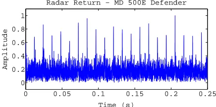
In order to make the algorithm independent of the initial position of the blades, the instantt0= 0is synchronised with the first flash,that is spike, of the received signal|y(t)˜ |. Figure
0 0.05 0.1 0.15 0.2 0.25 0
0.2 0.4 0.6 0.8 1
Radar Return − MD 500E Defender
Time (s)
[image:2.612.336.554.274.382.2]Amplitude
Figure 1. Example of the magnitude of a simulated radar signal received from an MD 500E Defender helicopter withSN R=−5dB.
1 shows an example of simulated signal received from an MD 500E Defender; it is clear that the flashes are still visible even at low SNR. The instant t? where the first flash is located, is obtained by evaluating a threshold η and identifying the first instant where the signal reaches such a threshold. Thus:
t?= arg min
t
|y(t)˜ | s.t. |y(t)˜ |> η. (12) The threshold η depends on the statistical characteristics of the received signal. Assuming an additive white Gaussian noise (AWGN) scenario,|y(t)˜ | has a Rice probability density function (PDF). Since the tail of the PDF is due to the higher amplitude of the flashes compared to the noise, ηis computed as the 99.5%quartile of the distribution. Thus:
F|˜y|(η) = 0.995 (13)
whereF|y˜|(α)is the Cumulative Distribution Function (CDF)
of |y(t)˜ |. Accordingly, the atoms in (11) are synchronised by choosing φ=π/2.
B. Estimation ofζ
The estimation of ζ is the core of the algorithm and it is explained in this section. The letter l indicates the counter;
r(l)(r, o) and xˆ(l)
K(r, o) are the recovery residual and the
estimate of the vector x(Kl)(r, o), respectively, at iteration l;
Λ(l)(r, o)is the set of selected atoms;Φ(l)
Λ(r, o)is the matrix
0) Initialization: l = 1, xˆ(0)K (r, o) = 0, r(0)(r, o) = ˜y,
Λ(0)(r, o) =∅,Φ(0)
Λ(r, o) =0.
1) For each couple (r, o)
1.1) The inner product between the residual at the previous step,r(l−1)(r, o), and the blockΨK(r, o)
of the dictionary is carried out and stored in p:
p= D
ΨK(r, o),r(l−1)(r, o)
E
. (14)
1.2) ˆi indicates the location of the maximum value of
p:
ˆi= arg max
i
p(i), (15)
which is then added to the setΛ(l)(r, o):
Λ(l)(r, o) =Λ(l−1)(r, o)∪ˆi. (16) 1.3) Φ(l)
Λ(r, o)is updated accordingly to the new set of
selected atoms Λ(l)(r, o).
1.4) The estimate of the vector x(Kl)(r, o)is performed as solution of a least square problem:
ˆ
xK(l)(r, o) =hΦΛ(l)(r, o)HΦ(Λl)(r, o)i −1
Φ(Λl)(r, o)Hy˜.
(17) 1.5) The residual is updated as:
r(l)(r, o) = ˜y−Φ(l) Λ(r, o)ˆx
(l)
K(r, o). (18)
2) Remove O
2
candidate values from O, which corre-spond to the largest residual errorr(l)(r, o)
, wherek·k indicates the`2-normof the vector. At thel-th cycle, the number of couples (r, o)is thenR×O
2l
. 3) If O2l
> 1, increment l and return to the step 1, otherwise go to step 4.
4) Since O has only one value left, whose index is ˆo, this represents the estimated angular velocity of the target,
ˆ
ω=ω(ˆo). Moreover, let˜lbe the last value of the counter at this stage;ρˆis equal to:
ˆ
ρ=ρ(ˆr), (19)
where:
ˆ
r= arg min
r r
(˜l) (r,o)ˆ
. (20)
5) Repeat the step from 1.1) through 1.5) K times, withrˆ
andoˆin place ofrando, respectively, and the following initial values: l = 1, xˆ(0)K (ˆr,o) =ˆ 0, r(0)(ˆr,o) = ˜ˆ y,
Λ(0)(ˆr,o) =ˆ ∅,Φ(0)Λ(ˆr,o) =ˆ 0.
6) Let˜l be the last value of the counter at this stage, then:
ˆ
κ=κ(ˆk), (21)
where:
ˆ
k= arg max
k xˆ
(˜l) K(ˆr,ˆo)
=
arg max
k
[|xˆ0,r,ˆoˆ|, . . . ,|xˆk,r,ˆoˆ|, . . . ,|xˆK−1,r,ˆˆo|], (22)
completes the estimation process.
C. Classification
At the end of the first two stages the state vector ˆζ = (ˆκ,ρ,ˆ ω)ˆ is estimated. Let h0, . . . ,hV−1 be the triples which represent V known helicopters, the classification is obtained by computing a weighted Euclidian distance:
ˆ
v= arg min
v
ˆ
ζ−hv T
s
, (23)
wheresis the vector of the weights.
IV. EXPERIMENTALRESULTS ONSIMULATEDDATA
The algorithm is tested by means of simulated data. For different values of the SNR,90trial radar signals with a carrier frequency of 5 GHz are generated by using the equation (1),
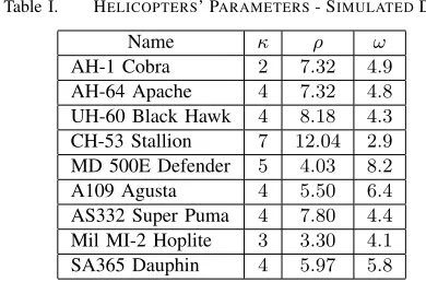
[image:3.612.339.534.254.383.2]10 for each target listed in Table I. The initial phase φ and
Table I. HELICOPTERS’ PARAMETERS- SIMULATEDDATA
Name κ ρ ω
AH-1 Cobra 2 7.32 4.9 AH-64 Apache 4 7.32 4.8 UH-60 Black Hawk 4 8.18 4.3 CH-53 Stallion 7 12.04 2.9 MD 500E Defender 5 4.03 8.2 A109 Agusta 4 5.50 6.4 AS332 Super Puma 4 7.80 4.4 Mil MI-2 Hoplite 3 3.30 4.1 SA365 Dauphin 4 5.97 5.8
the aspect angle β are considered unknowns and are chosen randomly, in particular the latter ranges in [0◦,70◦]. The duration of the signals is chosen such that at least a complete rotation period is contained; considering the minimum product between the first and the third column, it is assumed equal to
0.25 seconds. Furthermone, it is supposed to have a system with a pulse repetition frequency (PRF) able to cope with the
maximum expected Doppler shift; in this case, since:
fmD,max= 2
2πmax(ωρ)
λ , (24)
it is chosen equal to8 kHz.
The dictionaryΨis built by choosing the following alpha-bets:
K={2,3,4,5,6,7}, (25)
R={3.5,4,4.5, . . . ,12.5}, (26)
O={2.5,2.6,2.7, . . . ,8.5}. (27) withβandR0equal to70◦andλ/16, respectively.The choice of such a smallR0 must not surprise, since it only appears in the factorexp−j4λπR0 in (1), which is periodic; moreover, it is easy to verify that the real and the imaginary part of that
complex term is zero when R0 = λ8 ±m4λ andR0=±mλ4,
respectively, where m is any non-negative integer. For this
reason, regarding the design of the dictionary, it is chosen equal toλ/16.
The classification is performed by computing a weighted Euclidian distance with the following weights:
This choice is made in order to penalise the estimates of ρ
andκ, which are the most affected by the noise. In particular
ˆ
ρ is weighted by 0 because, as shown in (1),ρ appears both as a real multiplicative factor and multiplied by cosβ. In the first case, the information is lost since the algorithm is made independent of the RCS through (10) and (11), besides it is affected by the additive noise. In the second case, since β
is unknown, even the product ρcosβ is unknown, hence its estimate is not reliable. However, it has to be kept in the model in order to evaluate both κˆ andωˆ.
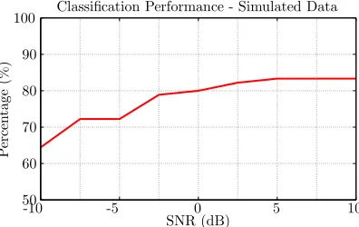
The performance in terms of percentage of correct classi-fication is shown in Figure 2. Even at SN R=−7.5 dB, the helicopters are correctly classified in the 72.22%of the cases. For values of the SNR above 0 dB, the percentage of correct classification is above80%.
Classification Performance - Simulated Data
SNR (dB)
P
er
ce
n
ta
ge
(%
)
-10 -5 0 5 10
[image:4.612.354.535.65.113.2]50 60 70 80 90 100
Figure 2. Performace on simulated data in terms of percentage of correct classification.
Table II shows the confusion matrix atSN R= 0dB. AH-64, MI-2 and CH-53 present the highest mismatch rates. The first two are mostly confused with AH-1 and UH-60, respectively, and this is likely due to their similar rotation speeds, while the last one is confused with SA365. However, 6 out of 9
[image:4.612.74.272.229.354.2]helicopters present a percentage of correct classification higher than95%.
Table II. CONFUSIONMATRIX: RESULTS ONSIMULATEDDATA AT
SN R= 0dB.
AH-1 AH-64 UH-60 CH-53 MD
500E
A109 AS332 MI-2 SA365
AH-1 9 0 0 1 0 0 0 0 0
AH-64 3 5 0 1 0 1 0 0 0
UH-60 0 0 10 0 0 0 0 0 0
CH-53 0 0 0 4 0 0 0 1 5
MD-500E 0 0 1 0 9 0 0 0 0
A109 0 0 0 0 0 10 0 0 0
AS332 0 0 0 0 0 0 10 0 0
MI-2 0 0 5 0 0 0 0 5 0
SA-365 0 0 0 0 0 0 0 0 10
V. EXPERIMENTALRESULTS ONREALDATA
The validity of the approach is proved with real data. Signals from the two-bladed helicopter scale model GAUI X3 are acquired with a 24 GHz Continuous Wave (CW) radar, whose sampling frequency is22kHz. Three rotation speeds are chosen,in order to simulate as many targets A, B and C; their
actual values are not available, hence they are evaluated by
inspection of the time domain signals and the obtained values are shown in Table III, along with the standard deviations of
Table III. SCALEMODEL’SROTATIONSPEED
Target Actual Speed Standard Deviation
A 6.72rps 0.07
B 9.12rps 0.05
C 12.42rps 0.15
the estimates. The database which contains the parameters of
the helicopters to classify is shown in Table IV; targets from D to L present either equal rotation speeds but different number of blades or the same number of blades with similar rotation speeds of the true targets A, B and C, in order to test the reliability of the algorithm. Accordingly to this choice, the dictionaryΨ is designed with the following alphabets:
K={2,3,4}, (29)
R={0.30,0.31, . . . ,0.40}, (30)
O={6.50,6.51,6.52, . . . ,13}. (31) Without loss of generality, a non-uniform sampling strategy is used for the alphabet O, denser in the neighbourhood of the expected values. As before, β is70◦,R0 isλ/16 and the weight vectorsis chosen equal to (28). With these values, the signal length and the sampling frequency are chosen equal to
0.4 seconds and5.5kHz, respectively.
Table IV. HELICOPTERS’ PARAMETERS- REALDATA
Target κ ω
A 2 6.72rps B 2 9.12rps C 2 12.42rps D 3 6.72rps E 3 9.12rps F 3 12.42rps G 4 6.72rps H 4 9.12rps I 4 12.42rps J 2 7.92rps L 2 10.77rps
Three acquisitions are made for each speed, at three different aspect anglesβ˜. From each signal, whose total length is 20 seconds, 50 segments of0.4 seconds are extracted and downsampled with a factor of4in order to match the sampling frequency of 5.5kHz.
[image:4.612.392.500.345.495.2]The performance is shown in Table V in terms of percent-age of correct classification. For β˜ = 0◦ the performance is
Table V. PERFORMANCE- REALDATA
Target β˜= 0◦ β˜= 30◦ β˜= 60◦
A 50% 100% 100%
B 68% 100% 100%
C 52% 82% 96%
lower than the other two cases because of the small RCS of the blades; however, this is an unlikely scenario since it means that the helicopter is flying at the same altitude of the radar. For values ofβ˜equal to30◦ and60◦, the correct classification
[image:4.612.63.278.470.619.2] [image:4.612.363.527.588.650.2]VI. CONCLUSION
In this paper a novel model-based automatic classification algorithm for helicopters was presented. A sparse signal model for radar return from a helicopter was designed and used in conjunction with a greedy sparse signal recovery algorithm to extract the micro-Doppler parameters of the target. The latter were then used to perform the classification by simply comparing them with micro-Doppler parameters of known helicopters. Unlike other approaches, the proposed algorithm does not need the computation of any time-frequency distri-bution, which makes it independent of the dynamic of the received signal, and presents a low computational cost since the dictionary can be pre-computed based on the database of expected targets. Moreover, this method is independent of both the initial position of the blades and the inclination of the helicopter with respect to the LOS. The algorithm was tested by using both simulated and real data. The experimental results on simulated data show the capability of the algorithm of classifying the targets independently of both the initial phase of the signal and the aspect angle. The results obtained on real data confirm the validity of the approach, leading to an average
96% of correct classification in the cases of most interest.
ACKNOWLEDGMENT
This work was supported by the Engineering and Phys-ical Sciences Research Council (EPSRC) Grant number EP/K014307/1 and the MOD University Defence Research Collaboration in Signal Processing.
Gang Li’s work was supported in part by the National Natural Science Foundation of China under Grants 61422110 and 41271011, and in part by the Tsinghua University Initiative Scientific Research Program.
The authors would like to thank Mr. Jianlin Cao for making available the scale model helicopter used for the acquisitions of real data.
REFERENCES
[1] H.-T. Tran, R. Melino, P. Berry, and D. Yau, “Microwave radar imaging of rotating blades,” inRadar (Radar), 2013 International Conference on, Sept 2013, pp. 202–207.
[2] C. Clemente, A. Balleri, K. Woodbridge, and J. Soraghan, “Devel-opments in target micro-Doppler signatures analysis: radar imaging, ultrasound and through-the-wall radar,”EURASIP Journal on Advances in Signal Processing, vol. 2013, no. 1, 2013.
[3] T. Thayaparan, L. Stankovi, and I. Djurovi, “Micro-Doppler-based target detection and feature extraction in indoor and outdoor environments,”
Journal of the Franklin Institute, vol. 345, no. 6, pp. 700–722, 2008. [4] L. Pallotta, C. Clemente, A. De Maio, J. Soraghan, and A. Farina,
“Pseudo-Zernike moments based radar micro-Doppler classification,” inRadar Conference, 2014 IEEE, May 2014, pp. 0850–0854. [5] J. Misiurewicz, K. Kulpa, and Z. Czekala, “Analysis of recorded
helicopter echo,” in Radar 97 (Conf. Publ. No. 449), Oct 1997, pp. 449–453.
[6] J. Martin and B. Mulgrew, “Analysis of the theoretical radar return signal form aircraft propeller blades,” in Radar Conference, 1990., Record of the IEEE 1990 International, May 1990, pp. 569–572. [7] C. Clemente and J. Soraghan, “GNSS-Based Passive Bistatic Radar for
Micro-Doppler Analysis of Helicopter Rotor Blades,” Aerospace and Electronic Systems, IEEE Transactions on, vol. 50, no. 1, pp. 491–500, January 2014.
[8] T. Thayaparan, S. Abrol, E. Riseborough, L. Stankovic, D. Lamothe, and G. Duff, “Analysis of radar micro-Doppler signatures from ex-perimental helicopter and human data,”Radar, Sonar Navigation, IET, vol. 1, no. 4, pp. 289–299, Aug 2007.
[9] V. Chen,The micro-Doppler Effect in Radar, 1st ed. Artech House, 2011.
[10] D. Donoho, “Compressed Sensing,”Information Theory, IEEE Trans-actions on, vol. 52, no. 4, pp. 1289–1306, April 2006.
[11] J. Tropp and A. Gilbert, “Signal Recovery From Random Measurements Via Orthogonal Matching Pursuit,”Information Theory, IEEE Transac-tions on, vol. 53, no. 12, pp. 4655–4666, Dec 2007.