Radial basis function (RBF)-based interpolation and spreading for the immersed boundary method

City, University of London Institutional Repository

Citation

:

This is the accepted version of the paper.

This version of the publication may differ from the final published

version.

Permanent repository link:

Link to published version

:

Copyright and reuse:

City Research Online aims to make research

outputs of City, University of London available to a wider audience.

Copyright and Moral Rights remain with the author(s) and/or copyright

holders. URLs from City Research Online may be freely distributed and

linked to.

Radial Basis Function (RBF)-based Interpolation and

Spreading for the Immersed Boundary Method

Francisco Toja-Silvaa,b,∗_{, Julien Favier}c_{, Alfredo Pinelli}d

a

Centro de Investigaciones Energ´eticas, Medioambientales y Tecnol´ogicas (CIEMAT), Av. Complutense 40, 28040 Madrid, Spain.

b

Escuela T´ecnica Superior de Ingenieros Aeron´auticos, Universidad Polit´ecnica de Madrid (UPM), Madrid, Spain.

c

Aix Marseille Universit´e, CNRS, Centrale Marseille, M2P2 UMR 7340, France.

d

School of Engineering and Mathematical Sciences (SEMS), City University London, EC1V 0HB London, United Kingdom.

Abstract

Immersed boundary methods are efficient tools of growing interest as they allow to use generic CFD codes to deal with complex, moving and deformable geometries, for a reasonable computational cost compared to classical body-conformal or unstructured mesh approaches. In this work, we propose a new immersed boundary method based on a radial basis functions frame-work for the spreading-interpolation procedure. The radial basis function approach allows for dealing with a cloud of scattered nodes around the im-mersed boundary, thus enabling the application of the devised algorithm to any underlying mesh system. The proposed method can also keep into ac-count both Dirichlet and Neumann type conditions. To demonstrate the capabilities of our novel approach, the imposition of Dirichlet boundary con-ditions on a 2D cylinder geometry in a Navier-Stokes CFD solver, and the imposition of Neumann boundary conditions on an adiabatic wall in an un-steady heat conduction problem are considered. One of the most significant advantage of the proposed method lies in its simplicity given by the algo-rithmic possibility of carrying out the interpolation and spreading steps all together, in a single step.

Keywords: Immersed-Boundary Method, Interpolation-Spreading, Radial Basis Functions.

1. Introduction

When considering complex geometries, immersed boundary (IB) methods constitute an efficient alternative to avoid either difficult or even impossible grid generation procedures when dealing with body-fitted formulations or extra computational costs associated with unstructured grid solvers. Those difficulties associated to classical body fitted or unstructured solvers, be-come even more severe for moving or deformable boundary, as is the case in fluid-structure interaction problems. Moreover, in those cases, the immersed boundary methods are not restricted to small boundary displacements such as other techniques based on smooth mesh deformation [1]. An alternative to immersed boundary methods is the immersed finite element method (IFEM) proposed by Zhang et al. [2]. This work extends the idea of the discrete Delta functions to unstructured meshes using the idea of Reproducing Ker-nel Particle Methods (RKPM). Both fluid and solid domains are modeled with finite element methods and the continuity between the fluid and solid sub-domains are enforced via the interpolation of the velocities, and the dis-tribution of the forces with the reproducing kernel particle method (RKPM) Delta function. The immersed boundary method was historically introduced by Peskin [3], in a pioneering work focussed on heart dynamics. Since then it has continuously evolved to tackle numerical simulations of new scien-tific domains, from biomedical to chemical engineering and aeronautics. The classical approach is to solve the problem equations on a uniform cartesian grid (Eulerian) for both solid and fluid phases. The boundary of the solid is described through a set of markers (Lagrangian) which do not coincide with the fluid mesh points. The communications between fluid and solid is done through volume forces that enforce the no-slip boundary condition and ensure the conservation at the wall of linear momentum, force and torque by means of interpolation-spreading operators (discrete Delta functions in the case of the classical method). Using the same discrete Delta functions for both interpolation and spreading guarantees conservation of energy, along with conservation of force and torque [4].

sharp boundaries and rigid objects [5]. The second group termed as “discrete forcing” methods [8, 12, 13, 14, 15, 16] is based on a set of singular body forces, defined on the Eulerian fluid nodes, to enforce the desired boundary values. This second group of techniques allows to use larger time-steps and, certain formulations, can handle sharp boundaries too [14]. The immersed boundary method that is proposed in the present work, which makes use of radial basis functions (RBFs), can be classified within the second group.

[17] present a direct forcing method based on compact integrated radial basis functions, using a smoothed version of the discrete delta functions to trans-fer the physical quantities between Eulerian and Lagrangian nodes. Shankar et al. [18] use RBF-based symmetric Hermite interpolation to extend the Augmented Direct Forcing method [16] to handle objects with concavities or objects in close proximity. This modified version of the Augmented Di-rect Forcing method was used in conjunction with an RBF-FD method for solving reaction-diffusion equations on object surfaces. Their method only requires the coordinates of the scattered nodes representing the surface and its normal-to-the-surface vectors at those locations.

In the present work we propose an original immersed boundary method based on radial basis functions interpolation. To the best of our knowledge, the method differs from previous literature implementations, proving to be easier to implement and more versatile than existing ones. The most signifi-cant advantages of the present method are: i)it is aplicable to any underlying grid system because based on an interpolation-spreading process defined on a scattered cloud of nodes; ii) the weights of the RBF are calculated in-dependently from the velocity of the nodes (i.e., for static geometries they only depend on the geometry); and, iii)both interpolation and spreading (or convolution) are carried out simultaneously in a single stage.

The paper is organised as follows: firstly, the formulation of the RBFs used within the IB algorithm is presented; next, the numerical algorithm that we envisaged to impose Dirichlet boundary conditions is presented and validated in the context of a 2D Navier-Stokes solver. Afterwards, the im-position of Neumann boundary conditions is discussed and applied in the case of a 2D unsteady heat conduction problem. Finally, conclusions and recommendations for further future works are given.

2. RBF interpolation from an arbitrarily scattered set of nodes

Following the basic idea behind immersed boundary methods, we define a set ofLagrangiannodesXi, i= 1· · ·mon the immersed surface Γ surrounded

by a cloud of neighbouring nodes (Euleriannodes) xk, k = 1· · ·n, belonging

to the underlying fluid grid. The key idea of the IB method is to compute the fluid velocity at nodes Xi viainterpolationfrom thexk, and thus find the set

of localised forces (per unit mass, and unit time) on the interface that restore the desired velocity condition on Γ. Typically, this set of singular forces Fi,

(spreading) operation, obtaining a set of Eulerian forcesfk, k= 1· · ·n. More

details on how this procedure has been adapted to the present algorithm will be illustrated later on. Here, we just highlight that one of the key ingredients of any IB method is the transfer of a force field from the Lagrangian to the Eulerian nodes and viceversa [4, 35]. We will write the relationship between the force defined on the immersed surface and the one acting on the fluid as:

F =W f, withF = (F1, F2,· · · , Fn)T and f = (f1, f2,· · · , fm)T (1)

whereW is a transformation matrix with mrows and ncolumns (in general,

n 6=m) which entries depend on the basis functions used for the interpolation. The W matrix must obey the constraint of having all its column-sum equal to unity to conserve the total force, Pm_i=1Fi = Pn_k=1fk, and to guarantee

energy conservation (i.e., the work done by the forces in the two grid systems, see [20, 21]). Indeed if P_iWi,k = 1, we have:

X

i

Fi =

X

i

X

k

Wi,kfk=

X

k

fk

X

i

Wi,k=

X

k

fk (2)

Thus, the column-sum of W must be equal to unity independently of the interpolatory technique that is used. Next, we assemble matrix W making use of RBFs also introducing theinverseoperator that transfer the force data from the immersed interface to the fluid grid. We start by writing one of the equations of (1), that provides the interpolated value on a point Xl of the

immersed surface as a function of the n values on the fluid grid:

Fl = n

X

j=1

ωjfj, withFl =F(Xl) andfj =f(xj) (3)

where ωi, i = 1,· · ·n are unknown interpolation weights. To determine the

values of the weights, we rewrite (3) as:

Fl = n X j=1 " _n X k=1

λj,kφ(kXl−xkk) +γj

#

| {z }

ωj

fj, (4)

Where φj,k = φ(kxj −xkk) is a radial basis function: a symmetric function

To determine the value of the unknown parameters λj,k and γj (and thus of

ωj), for each node xj, j = 1,· · · , n we impose the cardinality conditions: n

X

k=1

λj,kφj,k+γj =δj,k (5)

(whereδj,k is the usual Kroeneker symbol) together with the constraint that

the interpolant should exacly represent a constant function Pn_k=1λj,k = 0.

Thus, for each node of the support x_j, we need to solve a linear system of equations to determine the λj,k, k = 1· · ·n:

       

φ1,1 · · · φ1,n 1

· · · · φj,1 · · · φj,n 1

· · · · φn,1 · · · φn,n 1

1 · · · 1 0

               

λj,1

· · · λj,j · · · λj,n γj         =         0 · · · 1 · · · 0 0         (6)

For the present work we have used the inverse multiquadric radial basis functions (IMQ-RBF):

φj,k ≡φ(rj,k) := {

1

p

1 + (ǫrj,i)2

:j, k ∈ ℑl}, rj,k =kxj −xkk (7)

where ℑl denotes the interpolation support of node Xl (that is discussed in

detail later),ǫ >0 is the shape parameter andrj,k the radial distance between

the nodes j and k. Note that φi,i = 1. The optimum value of the shape

parameterǫdepends on the noise in the data set, and it has to be determined according to each application. In summary, by solving the linear systems formed by Eqs. (6) we determine the weights λj,k that are independent on

the location of Xl. Next, we compute the ωj by evaluating the expression

ωj = Pnk=1λj,kφ(kXl −xkk) +γj to be used in the interpolatory formula

(3). By considering all the Lagrangian pointsX_l, and thus all the respective Eulerian support ℑl, we can compute all the weights ωj that correspond to

the entries of matrix W appearing in (1).

An important feature of this interpolant is that the weightsλj,kcan be also

used to approximate the value of the derivative (or of any linear differential operator L(f)) at the Lagrangian nodel. Indeed, we have:

L(f)(Xl) = n X j=1 n X k=1

WhereL(φ)(kX_l−x_kk) is the linear differential operator applied to the IMQ-RBF evaluated in Xl.

In the particular case of the normal derivative to the immersed boundary Γ at point X_l where the unit normal vector is ~n and the tangent vector is given by ~τ = [τx, τy]T, one can define the linear differential operator via

the projection P = I−τ τT _{(where I is the identity matrix). Using P, the}

approximation to the normal derivative of a functionf atXl= (xl, yl) reads:

L(f)(X_l) =∇f~ ·~n=

n

X

j=1 n

X

k=1

P ~∇φ(kX_l−x_kk)fj (9)

with ∇φ~ (kXl−xkk) = (∂xφ(kXl−xkk), ∂yφ(kXl−xkk))T and:

∂xφ(kXl−xkk)≡ −

ǫ2_(x

l−xk)

(1 + (ǫrl,k)2)3/2

, (10)

∂yφ(kXl−xkk)≡ −

ǫ2_(y l−yk)

(1 + (ǫrl,k)2)3/2

, (11)

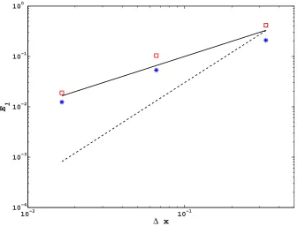
i.e., the partial x and partial y derivatives of (7). The convergence order of the IMQ-RBF depends on both the smoothness of the target function and the node density of the data sites. For smooth target functions that lie in its native space, the IMQ-RBF can exhibit spectral convergence. For a full discussion, see [26]. In the present case, described in §3.1, the interpolation functions have a first order convergence rate. The order that can be achieved is mainly related with the support used for the interpolation. Figure 1 shows the norm of the interpolation errorERBF at the immersed surface defined by

ERBF = max

l {URBF}, (12)

where URBF refers to the interpolation error of an arbitrary known field at

each Lagrangian point l (difference between the interpolated value and the known function at the point). The given results correspond to the method and the support choice described in the next section.

3. Imposition of Dirichlet boundary conditions

10−2 10−1 10−3

10−2 10−1 100

∆ x E RBF

Figure 1: Norm of the interpolation error at the Lagrangian points for the case described in §3.1. Red squares: interpolation error; solid line: ∆x (1st order); dashed line: ∆x2 _{(2nd order).}

example). In this framework, a popular time advancement procedure (as it is done in [8] for instance) reads as:

u∗_−un

∆t =−Nl(u

n_{, u}n−1_)−Gφn−1₊ 1

ReL(u

∗_{, u}n_{), (13)}

for the predicted momentum equation, and

Lφ= 1

∆tDu

∗_{, (14)}

for the value of the projector (i.e., the pseudo pressure) that enforces the divergence free condition via:

In the given, time discretised equations, u∗ _{is the predicted velocity field, u}n is the velocity field obtained at the time-stepn, ∆tis the time step,Nl,Gand

D are, respectively, the finite-difference discrete approximation of the non-linear, the gradient and the divergence operators,Lis the discrete Laplacian and φ is a projection variable (related to the pressure field). Normally, all those operators are defined on a staggered grid system [11].

To impose assigned Dirichlet boundary values on the immersed boundary Γ, the above time sequence is modified by carrying out the time advancement of the predicted momentum equations in two stages: Firstly, a fully explicit prediction step is performed without body force (without keeping into ac-count the Dirichlet values on Γ) by advancing Eq. (13). The predicted velocity field u∗ _{leads to a predicted force field u}∗_{/∆t (per unit mass), that} is interpolated on the immersed boundary using the procedure described in the previous section. Next, we determine the necessary force per unit mass required to enforce the desired boundary conditions on Γ.

F = U

o

∆t − I(u∗₎

∆t , (16)

In (16),Uo_{is the desired velocity distribution on the immersed boundary, and}

I is the interpolator operator (Eulerian mesh to immersed surface). Once the value of the restoring forceF on Γ has been determined, we seek corrections to the momentum equation, discretised on the Eulerian mesh, by introducing a set of singular body forces. In other words, we should determine the values of f to be assigned to the interpolating Eulerian nodes to recover the values of F on Γ given by (16):

f =R(u∗_{/∆t), (17)}

where R refers to the interpolation-spreading using a radial basis function. The regularized forcef is then added to the right hand side of the momentum equations, and the time advancement of Eq. (13) is repeated:

u∗_−un

∆t =−Nl(u

n_{, u}n−1_)−Gφn−1₊ 1

ReL(u

∗_{, u}n_{) +f. (18)}

3.1. Methodology

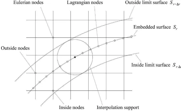
For sake of clarity, we consider Γ to be a circle of radius r, centred at (xc,yc). The Eulerian nodes neighbouring the immersed surface belong to a

an anulus of width 2∆r defined along the immersed boundary. The nodes enclosed in this region will be the ones involved with the interpolation and spreading operations (see figure 2). We start by tagging the inner nodes,

Figure 2: Diagram of the interpolation support.

adjacent to the embedded surface, using the following condition:

Sr−∆r <(xin, yin)< Sr, (19)

Similarly, the outer nodes satisfy:

Sr<(xout, yout)< Sr+∆r. (20)

where Sr+α is the circumference of a circle of radius r+α centred at (xc,yc).

For more general geometries, to tag the inner and outer nodes, one could resort to a level set function [28] (in the simple case of a circle given by

h(x, y) = (x−xc)2+ (y−yc)2−r2) and discriminate the position according to

an outer/inner location). The number of inner Eulerian nodes will also define the number of Lagrangian nodes used to discretise Γ. The same number will also define the size of the linear system to be solved for the interpolation-spreading process (i.e.,n, the size of matrixW of equation (1)). As explained in the following, if the number of Lagrangian nodes is equal to the number of inner Eulerian nodes, the resulting linear system will have the same number of equations and unknowns (square matrix). Other choices are possible if a least square approximation of the boundary values is seeked. In this case to improve the accuracy of the method, one should specify a number of Lagrangian nodes larger than the number of Eulerian nodes falling within the internal part of the anulus. The interpolation support is shown in figure 2. A number of numerical experiments has been performed considering different boundary layer thickness (i.e., Reynolds numbers of the flow around the circle) and different mesh sizes. Those numerical experiments suggest that a good compromise between stability and accuracy is attained for a number of Lagrangian nodes taken to be about three times the number of nodes in the inner region. The set of all inner points corresponds to the union of the interpolation supports of each Lagrangian node. The interpolation support for each one of them, is determined using another smaller circle centered on a point belonging to Sr and with a radius of ∆r. This circle is thus

tangent to both Sr+∆r and Sr−∆r (see figure 2). After a parametric study, the value of ∆r = ∆x has been found to be robust over variations of the Γ geometry (circular, elliptical, with sharp arcs, etc.). Both the inner Eulerian and Lagrangian nodes that fall within this circle, constitute the inner subset of the support that is used for the interpolation step.

Once the set of all the supports is defined, we proceed to interpolate the fluid velocity onto the Lagrangian nodes using a the compact radial basis function method described in the previous section. Firstly, we evaluate the weights ωj(Xl) using (6) in conjunction with (7). Concerning the value of

the parameter ǫ appearing in (7), we have found, via a parametric study, that the value ǫ=Re/∆x is a robust choice over variations of the Reynolds number Re. This point clearly requires further investigation. However, in this work, we simply use this empirically-determined value and found that it performs quite well in the ranger 25 < Re < 250. During our numerical experiments we have also systematically verified that the column-sum of all weigths in matrix W (i.e., equation (1)) is indeed equal to unity.

interpolation formula:

ul

∆t =ω1 u1

∆t +ω2 u2

∆t +...+ωn un

∆t. (21)

As previously mentioned, the fluid velocity is decomposed into an esti-mated velocity u∗ _{(computed by Eq. 13), and a regularized forcef imposing} the desired conditions on Γ. In the specific case of homogeneous Dirichlet conditions (no-slip: UXl = 0 on Γ), the merging of the interpolated values

with the unknown values on the support, leads to:

0 =ωi1(

u∗

i1

∆t +fi1) +...+ωin( u∗

in

∆t +fin) +ωo1 u∗

o1

∆t +...+ωon u∗

on

∆t. (22)

Equation (22) is an overdetermined system of linear equations W f = b, having the values of f at the internal support nodes as unknowns. The matrix W, and the right-hand-side of the system are given by:

W =       

ωi1(l1) 0 0 ωi4(l1) 0

0 ωi2(l2) 0 ωi4(l2) 0

..

. ... ... ... ...

ωi1(ln−1) 0 0 0 ωi5(ln−1)

0 0 ωi3(ln) 0 ωi5(ln)

       , (23) and b =        

−Pωiu ∗

i

∆t|l1 −

P ωou

∗

o

∆t|l1

−Pωiu ∗

i

∆t|l2 −

P ωou

∗

o

∆t|l2

...

−Pωiu ∗

i

∆t|ln−1 −

P ωou

∗

o

∆t|ln−1

−Pωiu ∗

i

∆t|ln−

P ωou

∗

o

∆t|ln

        (24)

As the matrixW is not necessarily squared, we use a classical least square method to compute the regularized force fi:

WTW f =WTb. (25)

This numerical issue can be fixed by assigning to those nodes the same ve-locity as the closest ones laying on Γ. In the case of non-regular grids, this normal distance can be computed as 0.1∆r, being ∆r the thickness of the in-terpolation support, which is defined according to the mean distance between the cells close to the embedded surface. Since the boundary is approximated as piecewise linear, the accuracy is hardly affected by dividing a segment into two parts [13]. According to Gibou et al. [27], this approach preserve second order accuracy when solving the Poisson equation in irregular domains.

3.2. Results and discussion

To validate the proposed methodology, we have considered the case of a flow around a circular cylinder of diameter D at two Reynolds numbers,

ReD = 30 and ReD = 185. Following the numerical settings of [8], the

dimensions of the domain are Lx = 49D in streamwise direction and Ly =

34Din the normal direction. The center of the cylinder is located at (x, y) = (9D,17D). The mesh spacing is ∆x= ∆y= 0.0576D (Cartesian mesh).

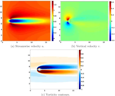
The no-slip boundary condition at the cylinder wall are imposed using the proposed algorithm. It is found that the methodology is able to reproduce successfully the characteristics of the flow at bothReD = 30 andReD = 185.

Figures 3 and 4 show the velocity fields and the vorticity contours. There is a qualitative agreement with the literature: at ReD = 30 the flow remains

steady with the presence of a recirculating region in the wake; atReD = 185,

periodic shedding vortices are formed downstream of the body (even if this case is nominally a 3D one since an instability in the spanwise direction should already be present, many authors have considered the 2D numerical study of the flow).

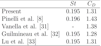
A more quantitative analysis is provided in Table 1 that shows compar-isons with the literature on the values of the main topological parameters of the wake at Re = 30 (see figure 5). Table 2 gives quantitative comparisons for the higher Re, unsteady case considering the values of the Strouhal num-ber and the drag mean coefficient obtained. A general good agreement is obtained, confirming the correct treatment of the boundary condition at the wall using the present method.

Figure 6 shows the norm of the interpolation error El at the immersed

surface defined by

El = max

l {Ul}, (26)

(a) Streamwise velocityu. (b) Vertical velocityv.

(c) Vorticity contours.

Figure 3: Mean velocity and vorticity contours atReD = 30.

l/D a/D b/D θ CD

Present 1.71 0.56 0.53 47.93 1.78

Pinelli et al. [8] 1.70 0.56 0.52 48.05 1.80 Coutanceau et al. [29] 1.55 0.54 0.54 50.00

-Tritton [30] - - - - 1.74

Table 1: Comparison of the main parameters of the wake and the drag coef-ficient at ReD = 30 with other works and experimental data.

(a) Streamwise velocityu. (b) Vertical velocityv.

(c) Instantaneous vorticity contours.

Figure 4: Instantaneous velocity and vorticity contours at ReD = 185.

St CD

Present 0.195 1.31

Pinelli et al. [8] 0.196 1.43 Vanella et al. [31] - 1.38 Guilmineau et al. [32] 0.195 1.28 Lu et al. [33] 0.195 1.31

Table 2: Comparison of the Strouhal number and the drag coefficient at

Figure 5: Shape parameters of the wake formed at Re= 30 [8].

4. Treatment of Neumann boundary conditions

We have tested the viability of our approach for imposing Neumann con-ditions by considering a simple 2D heat conduction equation around a ther-mically insulated cylinder.

Considering constant physical properties, and an implicit time advancing treatment, the governing equation of the heat conduction problem reads as:

Tn+1_−Tn

∆t =α∇

2_Tn+1_{, (27)}

where T is the temperature and α the thermal diffusivity, set to a value of α = 110·10−6_m2_{/s (which would correspond to copper thin plate). In} what follows, we describe the method by which Neumann conditions ∂T

∂~n = 0

are imposed at the immersed surface.

4.1. Methodology

10−2 10−1 10−4

10−3 10−2 10−1 100

∆ x E l

Figure 6: Norm of the interpolation error at the immersed surface for a Dirichlet boundary condition. Red squares: error u; blue asterisks: error v; solid line: ∆x (1st order); dashed line: ∆x2 _{(2nd order).}

nodes defining the immersed contour is more demanding for the case of Neu-mann conditions. We have found that the minimal number necessary to mantain the accuracy is about the double than the one required for imposing Dirichlet values.

As already mentioned, the use of radial basis functions for the interpola-tion of the derivative of the variable over the immersed boundary is a simple variation of the technique used for the interpolation of the values of the variable, thus rendering the method very friendly.

The first step is to evaluate the weights ωi of the function, applying the

following relationship between the Lagrangian node land each Eulerian node 1. . . n within the interpolation support:

φ~nl,2 =ω0+ω1φ2,1+ω2φ2,2+...+ωnφ2,n

...

φ~nl,n=ω0+ω1φn,1+ω2φn,2+...+ωnφn,n, (28)

where φi,j is the radial basis function between the node i and the node

j, and φ~nl,i is the derivative radial basis function between the l Lagrangian

node and the i Eulerian node projected on the normal surface direction ~n, as previously defined. By adding the extra condition: ω1+ω2+...+ωn = 0,

the following linear system of equations is obtained.

      

1 φ1,2 ... φ1,n 1

φ2,1 1 ... φ2,n 1

... ... ... ... ...

φn,1 φn,2 ... 1 1

1 1 ... 1 0

              ω1 ω2 ... ωn ω0        =       

φ~nl,1

φ~nl,2

...

φ~nl,n

0        . (29)

By interpolating the value of the temperatune normal derivative at each Lagrangian node as:

∂T

∂~n =ω1T1 +ω2T2 +...+ωnTn; (30)

and following the same methodology as for the Dirichlet case, we can write the equation:

0 =ωi1(Ti∗1+δi1) +...+ωin(Tin∗ +δin) +ωo1To∗1+...+ωonTon∗ , (31)

In (31),T∗

i is the temperature on the boundary without having imposed any

condition of the surface, and δi is the correction term to be applied to the

nodes inside the embedded surface.

Using the same algebraic manipulations as for the Dirichlet case, we fi-nally obtain the linear system W f =b, with

W =       

ωi1(l1) 0 0 ωi4(l1) 0

0 ωi2(l2) 0 ωi4(l2) 0

..

. ... ... ... ...

ωi1(ln−1) 0 0 0 ωi5(ln−1)

0 0 ωi3(ln) 0 ωi5(ln)

and b =       

−PωiTi∗|l1 −

P

ωoTo∗|l1

−PωiTi∗|l2 −

P

ωoTo∗|l2

...

−PωiTi∗|ln−1 −

P

ωoTo∗|ln−1

−PωiTi∗|ln−

P

ωoTo∗|ln

       (33)

Again, if W is not a squared matrix, the solution is found by resorting to a least square formulation: WT _{W δ = W}T _{b. We have found that}

the direct sum of the correction terms δi to the estimated temperatures Ti∗

induce a strong jump close to the immersed body. To avoid this problem, the correctionsδi are included in the governing equation of the problem (27)

instead. If Ti denotes the final (i.e., that keeps into account the Neumann

conditions) temperature field, the values T∗

i =Ti−δi are introduced into the

finite difference-discretized governing equation, obtaining:

aP(Ti,j −δi,j) +aS(Ti,j−1−δi,j−1) +aN(Ti,j+1−δi,j+1)+

aE(Ti+1,j−δi+1,j) +aW(Ti−1,j−δi−1,j) =b,

(34)

whereaI and bare the coefficients of the finite difference discretization of the

governing equation. Separating the unknowns in Eq. (34) yields:

aPTi,j+aSTi,j−1+aNTi,j+1+aETi+1,j +aWTi−1,j =

b+aPδi,j +aSδi,j−1+aNδi,j+1+aEδi+1,j+aWδi−1,j.

(35)

which, finally gives the linear system A T = b, where A is the same matrix as the first linear system that must be solved to obtain the estimated temperature field (i.e., standard finite difference Laplacian matrix).

4.2. Results and discussion

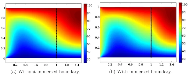
Following the procedure described above, we compute the temperature distrihution within a section of an infinitely long bar. The boundary on the right (east, E) is a perfectly insulated edge while the other three edges are maintained at a prescribed temperature value: TN = 100, TS = 25 and

TW = 75. Figure 7a shows the temperature field obtained for the whole

using our immersed boundary method. As expected, the temperature isolines approach the embedded surface in an orthogonal fashion (left hand side of the embedded surface).

(a) Without immersed boundary. (b) With immersed boundary.

Figure 7: Final temperature field T(x, y). External boundary conditions:

TN = 100, TS = 25, TW = 75 and the right hand side wall is considered

adiabatic.

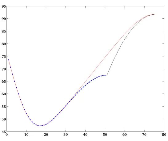
To complete the validation, the same problem has been tackled using a body conforming mesh. Figure 8 shows a longitudinal section in x direction at the center of the domain, where it can be seen that the results of both methodologies, body conformal (blue line) and immersed boundary using radial basis function (black line), fully agree.

Furthermore, figure 9 gives the values of the normal derivative of the temperature field just outside the vertical wall, using finite differences. The values of this parameter approach to zero (black squares) in front of the values without considering the adiabatic embedded surface (red circles).

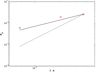
Figure 10 shows the norm of the interpolation errorEd at the immersed

surface defined by

Ed= max

l Ud, (36)

where Ud refers to the interpolated temperature derivative from the external

side computed at each Lagrangian point l. It results a decreasing of order ∆x (1st order).

Figure 8: Streamwise section of the temperature field at the center of the do-main. Red line: without considering the adiabatic embedded surface. Black line: considering the adiabatic embedded surface. Blue line: body conformal case.

5. Conclusions

In this work, we have presented a new interpolation and spreading proce-dure based on radial basis functions. The proceproce-dure is easy to implement and allows the imposition of both Dirichlet and Neumann boundary conditions. Both interpolation and spreading tasks are carried out together within the same stage, which yields a straightforward implementation. As the radial basis functions require a scattered cloud of points, another advantage is that the method works for any type of mesh, even unstructured.

To validate the method, a Dirichlet boundary condition has been imposed on a 2D cylinder geometry in a Navier-Stokes CFD solver, and a Neumann boundary condition has been imposed in an adiabatic embedded surface in an unsteady heat conduction problem. The obtained results agree with lit-erature results.

Figure 9: Normal derivative of the closest temperature field outside the verti-cal wall, in front of the height. Red circles: without considering the adiabatic embedded surface. Black squares: considering the adiabatic embedded sur-face.

increased by future works on the interpolation support. This new interpola-tion support should use more external nodes, since the first order accuracy derives from the order of the interpolation process. The most important challenge is to define a simple rule to select the appropriated nodes that will be able to deal with any surface shape.

10−2 10−4

10−3 10−2 10−1

∆ x E d

Figure 10: Norm of the interpolation error of the derivative at the immersed surface. Red squares: derivative error; solid line: ∆x (1st order); dashed line: ∆x2 _{(2nd order).}

is also a remaining issue, which is also encountered in other methods in literature.

Short-term applications of the work also includes the imposition of Neu-mann boundary conditions on the Poisson equation in a CFD code, and the use of the present method to implement wind turbine models such as actuator disc and actuator line ones.

6. Acknowledgments

(a) Without immersed boundary. (b) With immersed boundary.

Figure 11: Temperature field T(x, y). External boundary conditions: TN =

100, TS = 25, TW = 75 and TE = 50.

References

[1] L. Ji, K. Sreenivas, D. G. Hyams, R. V. Wilson. A parallel universal mesh deformation scheme for hydrodynamic applications. 28th Symposium on Naval Hydrodynamics, Pasadena (USA), 12-17 September 2010.

[2] L. Zhang, A. Gerstenberger, X. Wang, W. K. Liu. Immersed finite ele-ment method. Computer Methods in Applied Mechanics and Engineer-ing, 193 (2004): 2051-2067.

[3] C. S. Peskin. Flow patterns around heart valves: a numerical method. Journal of Computational Physics, 10 (1972): 252-271.

[4] C. S. Peskin. The immersed boundary method. Acta Numerica, 11 (2002): 479-517.

[5] R. Mittal, G. Iaccarino. Immersed boundary method. Annual Review of Fluid Mechanics, 37 (2005): 239-261.

[6] Z. Li, M. Lai. The immersed interface method for the Navier-Stokes equations with singular forces. Journal of Computational Physics, 171 (2001): 822-842.

[8] A. Pinelli, I. Z. Naqavi, U. Piomelli, J. Favier. Immersed-boundary methods for general finite-difference and finite-volume Navier-Stokes solvers. Journal of Computational Physics, 229 (2010): 9073-9091.

[9] J. van Kan. A second-order accurate pressure-correction scheme for vis-cous incompressible flow. SIAM Journal on Scientific and Statistical Computing, 7 (1986): 870-891.

[10] D. L. Brown, R. Cortez, M. L. Minion. Accurate projection methods for the incompressible Navier-Stokes equations. Journal of Computational Physics, 168 (2001): 464-499.

[11] J.H. Ferziger, M. Peric. Computational methods for fluid dynamics. 3rd Ed. (2002) Springer.

[12] E. A. Fadlun, R. Verzicco, P. Orlandi, J. Mohd-Yusof. Combined immersed-boundary finite-difference methods for three dimensional com-plex flow simulations. Journal of Computational Physics, 161 (2000): 35-60.

[13] Y. Tseng, J. H. Ferziger. A ghost-cell immersed boundary method for flow in complex geometry. Journal of Computational Physics, 192 (2003): 593-623.

[14] R. Mittal, H. Dong, M. Bozkurttas, F. M. Najjar, A. Vargas, A. von Loebbecke. A versatile sharp interface immersed boundary method for incompressible flows with complex boundaries. Journal of Computa-tional Physics, 227 (2008): 4825-4852.

[15] J. Lee, D. You. An implicit ghost-cell immersed boundary method for simulations of moving body problems with control of spurious force oscil-lations. Journal of Computational Physics, accepted manuscript (2012), doi: http://dx.doi.org/10.1016/j.jcp.2012.08.044

[17] N. Thai-Quang, N. Mai-Duy, C. D. Tran, T. Tran-Cong. A direct forcing immersed boundary method employed with compact integrated RBF ap-proximations for heat transfer and fluid flow problems. Computer Mod-eling in Engineering and Sciences, 96 (2013): 49-90.

[18] V. Shankar, G. B. Wright, A. L. Fogelson, R. M. Kirby. A radial basis function (RBF)-finite difference method for the simulation of reaction-diffusion equations on stationary platelets within the augmented forc-ing method. International Journal for Numerical Methods in Fluids, 75 (2014): 1-22.

[19] A. de Boer, M. van der Schoot, H. Bijl. Mesh deformation based on radial basis function interpolation. Computers and Structures, 85 (2007): 784-795.

[20] A. de Boer, A. van Zuijlen, H. Bijl. Review of coupling methods for non-matching meshes. Computer Methods in Applied Mechanics and Engineering, 196 (2007): 1515-1525.

[21] A. Beckert, H. Wendland. Multivariate interpolation for fluid-structure-interaction problems using radial basis functions. Aerospace Science and Technology, 5 (2001): 125-134.

[22] N. Mai-Duy, T. Tran-Cong. A Cartesian-grid collocation method based on radial-basis-function networks for solving PDEs in irregular domains. Numerical Methods for Partial Differential Equations, Wiley Online Li-brary, 23 (2007): 1192-1210.

[23] J. Fang, M. Diebold, C. Higgins, M. B. Parlange. Towards oscillation-free implementation of the immersed boundary method with spectral-like methods. Journal of Computational Physics, 230 (2011): 8179-8191.

[24] V. Shankar, G. B. Wright, R. M. Kirby, A. L. Fogelson. Augmenting the immersed boundary method with radial basis functions (RBFs) for the modeling of platelets in hemodynamic flows. arXiv preprint (2013), arXiv: 1304.7479.

[26] H. Wendland. Scattered data approximation. Cambrigde monographs on applied and computational mathematics. Cambridge: Cambridge Uni-versity Press, 2005.

[27] F. Gibou, R. P. Fedkiw, L. T. Cheng, M. Kang. A second-order-accurate symmetric discretization of the Poisson equation on irregular domains. Journal of Computational Physics, 176 (2002): 205-227.

[28] Z. Li, K. Ito. The immersed interface method. Numerical solutions of PDEs involving interfaces and irregular domains. Philadelphia: Society for Industrial and Applied Mathematics, 2006.

[29] M. Coutanceau, R. Bouard. Experimental determination of the main features of the viscous flow in the wake of a circular cylinder in uniform translation. Part 1. Steady flow. Journal of Fluid Mechanics, 79 (2) (1977): 231-256.

[30] D. J. Triton. Experiments on the flow past a circular cylinder at low Reynolds numbers. Journal of Fluid Mechanics, 6 (1959): 547-567.

[31] M. Vanella, E. Balaras. A moving-least-squares reconstruction for embedded-boundary formulations. Journal of Computational Physics, 228 (18) (2009): 6617-6628.

[32] E. Guilmineau, P. Queutey. A numerical simulation of vortex shedding from an oscillating circular cylinder. Journal of Fluids and Structures, 16 (6) (2002): 773-794.

[33] X. Y. Lu, C. Dalton. Calculation of the timing of vortex formation from an oscillating cylinder. Journal of Fluids and Structures, 10 (5) (1996): 527-541.

[34] E. J. Kansa. Multiquadrics-A scattered data approximation scheme with applications to computational fluid-dynamicsII solutions to parabolic, hyperbolic and elliptic partial differential equations. Computers & Math-ematics with Applications, 19 (1990): 147-161.