Numerical simulation of a collapsing bubble subject to gravity

City, University of London Institutional Repository

Citation

:

10.1063/1.4944561

This is the accepted version of the paper.

This version of the publication may differ from the final published

version.

Permanent repository link:

Link to published version

:

Copyright and reuse:

City Research Online aims to make research

outputs of City, University of London available to a wider audience.

Copyright and Moral Rights remain with the author(s) and/or copyright

holders. URLs from City Research Online may be freely distributed and

linked to.

Numerical simulation of a collapsing bubble subject to gravity

P. Koukouvinis 1,(a), M. Gavaises 1, O. Supponen 2, M. Farhat 2 1

City University London, Northampton Square, London EC1V 0HB, United Kingdom

2

EPFL-LMH, Avenue de Cour 33 Bis, CH-1007 Lausanne

Abstract. The present paper focuses on the simulation of the expansion and aspherical collapse of a

laser-generated bubble subjected to an acceleration field and comparison of the results with instances from high-speed videos. The interaction of the liquid and gas is handled with the Volume Of Fluid (VOF) method. Compressibility effects have been included for each phase to predict the propagation of pressure waves. Initial conditions were estimated through the Rayleigh Plesset equation, based on the maximum bubble size and collapse time. The simulation predictions indicate that during the expansion the bubble shape is very close to spherical. On the other hand, during the collapse the bubble point closest to the bottom of the container develops a slightly higher collapse velocity than the rest of the bubble surface. Over time, this causes momentum focusing and leads to a positive feedback mechanism that amplifies the collapse locally. At the latest collapse stages, a jet is formed at the axis of symmetry, with opposite direction to the acceleration vector, reaching velocities of even 300m/s. The simulation results agree with the observed bubble evolution and pattern from the experiments, obtained using high speed imaging, showing the collapse mechanism in great detail and clarity.

Keywords: Numerical simulation, compressible bubble dynamics, bubble collapse in pressure

gradient, interface capturing, cavitation.

I. INTRODUCTION

Traditionally, the dynamics of the bubble growth and collapse are described using the Rayleigh-Plesset equation1, 2, which is a simplified form of the Navier Stokes equations, applied in a spherically symmetric configuration. Even though modifications of the Rayleigh Plesset equation have been formulated over time, in order to address issues arising from simplifications in the original derivation, such as compressibility effects2, or bubble interactions3, still the main assumption of spherically symmetric bubble evolution remains.

In practice, bubbles are never perfectly spherical. Bubble development is very sensitive to the presence of asymmetries, manifested in the form of boundary presence (e.g. walls, free surfaces), external forcing terms and pressure gradients. It is notable that the developed asymmetry during the collapse of the bubble gives rise to the formation of jetting phenomena. There are many examples of both experimental and numerical studies illustrating the above effects. To be more specific:

The first experiments conducted on the behaviour of bubble/bubble clouds in the vicinity of boundaries (walls, free surfaces) that are publicly available, are by the US navy, see e.g. 4. The work of Benjamin and Ellis 5 is one of the first experimental works on a fundamental level to show high speed movies of the asymmetric collapse of bubbles in various configurations close and far from walls, showing the asymmetries during the collapse and the formation of microjets. Similarly, one of the first numerical works that have examined the influence of walls in the vicinity of collapsing bubbles is the pioneering work of Plesset and Chapman, who utilized the Marker-and-Cell method to track the interface of a collapsing bubble6; they have compared their results against another

experimental study, by Lauterborn and Bolle7. During the collapse, the bubble deformed in a non spherically symmetric way, with a jet formed towards the wall. A detailed literature review on past works on bubble interaction with boundaries can be found in the books of Brennen2, 8 and Leighton9. Later on, Mitchell and Hammitt10 studied the aspherical bubble collapse due to the influence of a constant pressure gradient, again with the Marker-and-Cell method. The review paper of Blake and Gibson11 discusses the advances in the analytical, experimental and numerical work conducted on the behaviour of bubbles in the vicinity of boundaries, such as rigid walls, deformable/flexible materials, liquid/liquid or liquid/gas interfaces.

In a continuing effort towards the understanding and prediction of cavitation erosion, works on the aspherical bubble collapse are still ongoing. Examples of such works on the fundamental level, are e.g. the work of M. Tinguely12, who investigated, among other subjects, the deformation of a bubble in the vicinity of a hydrofoil, due to the local pressure gradient. The important finding is that the local pressure field can dramatically affect the way of bubble collapse and the direction of the formed jet.

On the numerical side, various methodologies have been employed for the bubble description. One of the first methodologies, still being used for bubble clusters, is the Boundary Element Method, where only the surface of the bubble is discretized13; notable works are the work of Mendez et al. 14 focusing on the interaction of bubbles, or the work of Chahine et al.15 examining the deformation of the bubble and the interaction with the material at the wall in an effort to understand erosion damage due to microjet. Other notable examples are the work of Osterman et al.16, using the Volume Of Fluid (VOF) for simulating the bubble collapse in the vicinity of walls under the influence of acoustic fields, the work of Hawker et al.17, based on front tracking techniques for pressure wave interaction with bubble, and the work of Lauer et al.18, using level set methodology for simulating bubble configurations near walls.

In this work, the aspherical collapse of a laser-generated bubble due to the influence of an external acceleration field in initially stagnant water is examined with CFD techniques, aiming to replicate the experiments that have been conducted by EPFL in collaboration with ESA, as described in the work of Obresckow et al.19, 20. Briefly described here, the experiment consists of a spherical bubble, created in water contained in a cubic test chamber, using a green, high-power laser pulse. The ambient pressure level inside the test chamber is regulated with a vacuum pump and water is at room temperature. The external acceleration field can be the gravitation field of earth, or the apparent gravitational field experienced by the bubble under the flight conditions in the aforementioned experiments. In the simulations, the bubble interface is captured with the Volume Of Fluid (VOF) method and compressibility effects in both gas and liquid phases are included. Contrary to the work of Osterman et al.16, the Tait equation of state is used for the liquid, instead of a linearized one, since it is more accurate to the IAPWS data21, at extreme conditions. To the authors' knowledge no previous work has been done to predict the aspherical collapse of bubbles in presence of gravity with the VOF method, so this can be considered as a fundamental work examining the capability of current models to predict such configurations.

The main features that this work aims to replicate are the following:

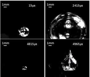
Figure 1. Evolution of the bubble shape, showing growth and collapse/rebound. Gravity acts at the vertical direction, towards the bottom. At rebound, an upwards moving jet is visible inside the bubble.

- The time evolution of the bubble size (quantitative): the bubble size can be estimated through the high speed images taken during experiments. Since the bubble may deform in a toroidal shape at its collapse, bubble size will refer to the instantaneously maximum diameter at the horizontal direction.

In previous experimental work conducted by EPFL, a non-dimensional scaling law, governing the collapse asymmetry and outcome, has been formulated as follows19:

v p p

R p

− ∇ =

∞

max

ζ (1)

where ∇p is the pressure gradient due to gravitational force, i.e. ρ⋅g , Rmax is the maximum bubble radius, p_∞ is the pressure at cavity level and pv is the vapour pressure. The higher the ζ value, the more pronounced the aspherical collapse and the jet volume is.

An extensive database of high speed videos and other measurements for different experimental conditions, including gravitational acceleration, is available at the EPFL website, conducted in collaboration with ESA, for ζ values ranging from 0 to 0.009 22. Additional experiments, conducted at EPFL facilities, are available also, with ζ values reaching up to 0.014. CFD simulations will aim to replicate selected bubble cases at different ζ values, ranging from zero to 0.014.

II. NUMERICAL MODEL

ignored. The equations solved, based on the compressible, viscous form of the Navier-Stokes equations 23, 24 using a commercial flow solver Fluent 16.125, are:

- Continuity equation:

( )

∇ + ∂ ∂ u

ρ

ρ

where u denotes the velocity vector of the flow field. - Momentum equation:

(

)

u_{+∇ ⊗ =−∇ +∇⋅ + +}

∂

∂

ρ

_ρ

_τ

_ρ

p

t (3)

where ρ is the density of the fluid, p is the pressure, g is the gravity vector, f are body forces and

τ

( )

[

∇

u

+

∇

u

]

+

( )

∇

⋅

u

I

=

µ

λ

τ

(4) In eq. 4, I is the identity matrix and µ is the dynamic viscosity of the fluid; for the pure phases it is set to 1mPa.s and 17.1µPa.s for water and air accordingly. Term λ denotes the bulk viscosity of the fluid which acts only on passing waves, commonly set to -2/3µ 23, 24, 26. The Reynolds number of the flow ranges from less than 1000, when the bubble is near maximum size, to even 90000 during the early expansion and latest collapse phases. However, for the majority of the simulation time, the Reynolds number is around 10000-20000. Due to the strong variation of the Reynolds number and its relatively low average value, that corresponds mainly to a transitional-mildly turbulent flow regime, it was chosen not to use any turbulence model.

Surface tension effects are included with the Continuum Surface Force model (Brackbill 27) as a volume force only in cells that are identified as an interface, i.e. where volume fraction varies between zero to unity.

- Volume fraction equation28:

+∇

(

)

∂ ∂ u G G a t

a

ρ

_ρ

(5)

where a represents the volume fraction and ρG the density of the gas phase. In the interface, where a varies from zero to unity, volume fraction averaging is performed for determining the value of viscosity and density.

Even if in the actual experiment there is significant influence of heating effects, due to laser interaction with the liquid, the resulting fluid state is not possible to describe with traditional equation of states, such as ideal gas or other, since plasma generation and reactions take place. As a compromise we chose to reduce the complexity of the thermodynamic model of the fluids involved and correlate pressure only to density. Even with the omission of thermal effects, both phases are assumed compressible, obeying the following equations of state:

- for the liquid, the Tait equation of state:

0 0 2 0 0 1 p n c p l n l +         −       = ρ ρ ρ ₍₆₎

where, ρ0 is liquid density, equal to 998.2kg/m

3

, c0 the speed of sound, equal to 1450m/s, at the reference state p0=2340Pa. The exponent nl is set to 7.15, according to relevant literature on weakly compressible liquids, such as water29.

- for the gas, a polytropic equation of state is used:

n

k

p= ρ (7)

process inside the bubble, e.g. for adiabatic it is equal to the heat capacity ratio and for isothermal it is unity. It is set close to unity, ranging from 1.025 to 1.125, depending on the case, see also Table I. As will be mentioned later, this is done based on trial-and-error basis, in order to fit the collapse time and maximum bubble size with the experimental data.

In order to minimize the effect of numerical diffusion, which could affect the development of the bubble during the whole process of growth and collapse, high order schemes have been used. To be more specific, second order upwind schemes have been used for the discretization of density and momentum, while the VOF phase field has been discretized using an implicit compressive differencing interface scheme 25, 30. Time stepping is done with an adaptive method, in order to achieve a Courant-Friedrichs-Lewy (CFL) condition 28 for the free surface propagation of 0.2; this is necessary to limit as much as possible the interface diffusion and maintain solution accuracy at the vicinity of the free surface 31. The solver used is implicit pressure based and this removes any restrictions on the acoustic Courant number, which is at maximum ~5, considering the minimum cell size and the maximum velocity. All the 2-phase simulations to be presented in the current work are set-up as 2D axisymmetric. The reasons for this selection are the axial-symmetry that dominates the whole phenomenon until the late stages of the rebound phase and the significantly reduced computational cost of an axisymmetric simulation in comparison to the full 3D simulation; just for reference, the simulations presented in the current work were conducted on a modern desktop computer over 2-3 days of computational time. If a full 3D simulation was to be pursued, then the computational cost would have been significantly higher, necessitating the usage of a cluster.

Apart from the solution of the 2-phase compressible Navier Stokes equations, a very useful tool for the estimation of the bubble expansion/collapse size and time evolution is the Rayleigh-Plesset equation. The standard Rayleigh-Plesset equation 1 was used, in the following form:

R R R R R p p p R R R n g v & & &

& σ _µ

ρ 2 4

2

3 ₀ 3

0

2 _ − −

     + − =    

+ ∞ (8)

where:

- ρ is the water liquid density, 998.2kg/m3 - R is the bubble radius,

dt dR

R& = and 2 2

dt R d R&&=

- pv is the vapour pressure.

-

p

- pg0 is the initial bubble pressure, tuned to predict a similar bubble evolution as the experiment. - σ is surface tension; here a value of 0.072N/m is used.

- µ is the dynamic viscosity of water, i.e. 1.01.10-3Pa.s

- n is a polytropic exponent, set close to unity as in the gas equation of state.

It has to be kept in mind that one of the main assumptions of the Rayleigh Plesset equation is the spherical bubble in an infinite liquid volume. It is clear that the main cases of interest are not perfectly spherically symmetric, due to e.g. the gravitational field, and in a bounded space, so one cannot expect a perfect match between the experiments or numerical simulations and the Rayleigh Plesset equation results. Still the Rayleigh-Plesset equation can assist both in the validation of the proposed methodology and in the set-up of the simulations to follow, since it can provide quick estimates of the bubble response for given initial conditions.

mass transfer through the bubble interface is fast enough so that the vapour pressure inside the bubble is always equal to saturation pressure.

III. VALIDATION OF THE METHODOLOGY

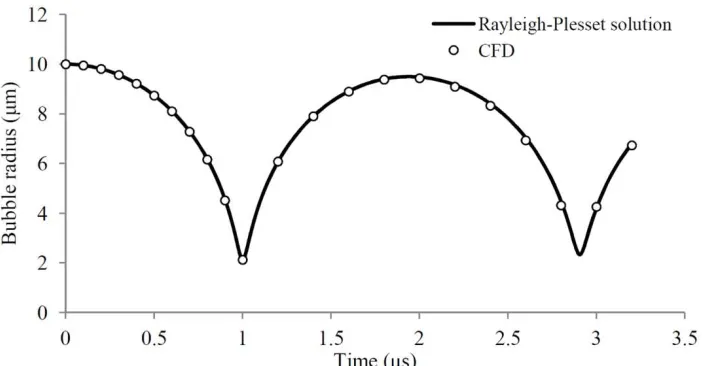
Before moving to complicated cases, with boundaries and complex bubble deformations, a preliminary study is conducted with the aforementioned methodology, in order to compare its predictions the Rayleigh Plesset equation. For this case, which corresponds to a ζ value of 0, the whole process of bubble growth and collapse is spherically symmetric. The bubble to be simulated corresponds to a case examined in the literature by Popinet et al., for more information see 32:

- the bubble has an initial radius of R0=10µm - the surrounding liquid pressure is

p

- the gas inside the bubble obeys an isentropic law with n=1.4 - the liquid density is 1000kg/m3 and dynamic viscosity 1mPa.s - surface tension coefficient is σ=0.07N/m

- amount of gas inside the bubble corresponds to equilibrium radius of 5µm 32; this corresponds to an initial pressure pg0 of ~6900Pa inside the bubble.

- there is no vapour inside the bubble (vapour mass transfer is omitted).

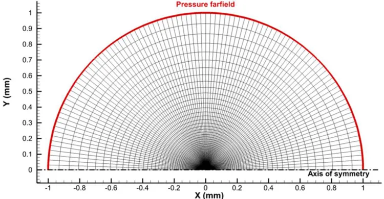
Since the configuration resembles a spherically symmetric collapse, a 2-dimensional axisymmetric computational domain was used to represent the bubble and the surrounding liquid; the domain resembles a half-circle, as shown in Figure 2, with the bubble centre placed at the origin (0, 0). The computational mesh is of O-grid type 33, to preserve the spherical symmetry of the bubble interface, limit numerical diffusion and prevent introduction of numerical artefacts. Note that the Navier-Stokes solution requires a finite computational grid, thus, to minimize the influence of the pressure far field, the boundary is placed 100 times the initial radius away from the bubble. Experience has shown that placing the boundary closer can lead to a dramatic underestimation in the collapse time of the bubble.

Figure 2. The computational domain and mesh for the validation case.

Figure 3. Bubble collapse evolution; comparison between the Rayleigh-Plesset equation and Navier Stokes solution.

Figure 4. Bubble collapse sequence for ζ=0 for the validation case. The thick black continuous line denotes the bubble interface and the dashed-dotted line the axis of symmetry.

IV. EXPERIMENTAL GEOMETRY AND COMPUTATIONAL MESH

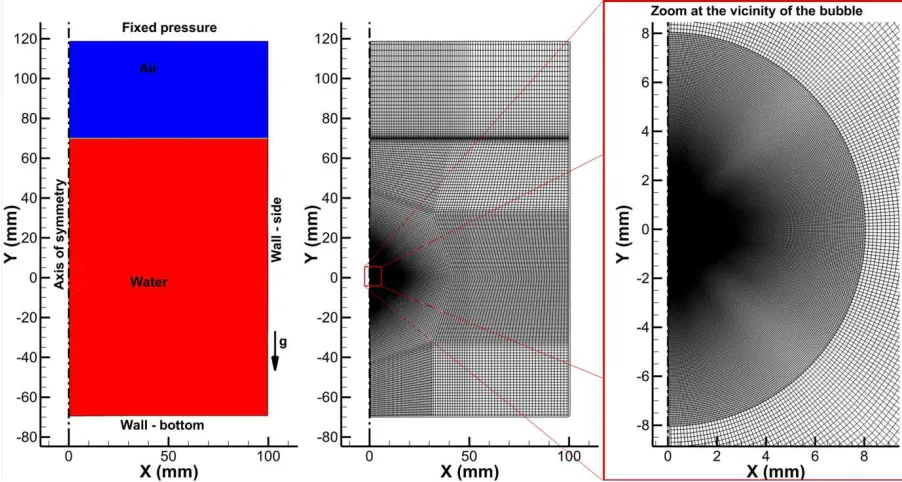
The computational domain simulated is based on the dimensions of the water container that has been used for parabolic flights 20, i.e. a box of inner dimensions 178.2x178.2x190.2mm (Width x Length x Height). Since the simulations are inherently 2D axisymmetric, a 2D rectangular domain of was used with the same cross-section as the original container, i.e. 100.5 x 190.2mm. Experience has shown that using a domain with the same cross-section as the actual container is essential for capturing the correct collapse of even the largest bubble, with Rmax~7.2mm (ζ~0.014).

The 2D rectangular domain was meshed with a block-structured strategy, with local refinement in the area of interest, which spans in a radius of 8mm around the origin; as with the validation case, the mesh in the vicinity of the bubble is of O-grid type. The aim of this refinement region is to capture with adequate resolution the bubble growth and collapse, without needing an excessive amount of computational elements in the whole container. This particular type of meshing ensures that as the bubble becomes smaller and smaller there will be enough elements to describe it, since the cell size decreases as one moves towards the centre of the bubble. Note that there is also refinement at the vicinity of the free surface, though not as fine as in the vicinity of the bubble, since the free surface deformation is not of interest in this study. The computational domain consists of 200000 cells and in the area of interest the cell size varies from 50µm to 0.4µm near the origin.

The container is initially filled with 140mm of water and the bubble is generated at 70mm from the bottom. The ambient pressure the experiments are conducted varies from 7500 to 10100Pa. This pressure is imposed at the fixed pressure boundary, depending on the case, and is initially set at the air region of the computational domain; the hydrostatic component of the air column is omitted since it is insignificant (the hydrostatic pressure of air is less than 0.1Pa at the experiment's ambient conditions, for a column of 50mm height). On the other hand, the water part is initialized with the hydrostatic pressure, since its contribution is not negligible. Gravitational acceleration is imposed as a momentum source term, depending on the exact value of the experimental conditions for each case.

Figure 5. Configuration used for the simulation. Left: the 2D computational domain used. Middle and right: the block-structured computational mesh with refinement in the area of interest.

A summary of the examined cases, with the main important conditions mentioned is highlighted below:

Table I. Conditions for the various test cases to be examined

Case pair

(Pa)

∆p

(Pa)

pv

(Pa)

Rmax

(mm)

g

(m/s2) Reference name

22

p

(Pa)

ζ

(.10-3)

1 8938 7190 2460 4.345 10.18 cavity124 9650 6.142

2 10174 8980 2460 4.549 18.12 cavity147 11440 9.162

The laser-generated bubble is introduced as a high pressure gas bubble, located at the same location as in the experiments, i.e. 70mm below the free surface. This is done by patching an amount of gas in a circular shape at the origin, initial radius R0 and initial pressure p0. Initial radius R0 is estimated based on the observed minimum radius during collapse; in all cases the bubble radius at the collapse is ~0.3-0.5mm. The initial bubble size has to be smaller than the bubble radius at collapse, considering the periodic nature of the Rayleigh Plesset equation in the absence of damping terms. On the other hand, a very small size would be both problematic to resolve and will impose very small time-stepping, in order to preserve accuracy of the interface. Thus, an initial radius of 0.1mm was chosen as an initial bubble size, since it was found adequate to give good predictions of the bubble evolution, while being computationally efficient to resolve.

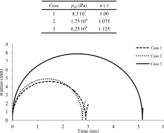
The initial bubble pressure is chosen so that the predicted bubble growth/collapse time and maximum radius matches the relevant from the experiments. This process is done in two stages: the first stage is by using the Rayleigh-Plesset equation, to quickly estimate approximate pressure levels that are needed in order to predict a similar bubble behaviour as in the experiments. It has to be kept in mind that the deviation from spherical symmetry and the existence of boundaries will render this initial pressure estimate somewhat inaccurate. For that reason, the second stage is using the described methodology in a trial and error basis until the maximum bubble radius is predicted appropriately. After going through this two stage methodology, the initial pressures and polytropic exponents shown in Table II have been determined (see also the predicted evolution of the bubble radius, using the Rayleigh-Pesset equation, in Figure 6). The variation of the polytropic exponent has a weak effect in the collapse time. If the same polytropic exponent of 1.05 was used in all cases, with appropriate initial pressure to reach the same maximum bubble radius, the deviation from the experimentally determined collapse times would increase by ~3% maximum.

Table II. Initial conditions for the various test cases to be examined

Case pg0 (Pa) n (-)

1 8.3.107 1.00

2 1.75.108 1.075

3 6.25.108 1.125

V. RESULTS

In this section, selected results of the aforementioned cases will be presented. Each figure is split at the middle, at the axis of symmetry. The left part of the figure shows the pressure field and the right the velocity magnitude. The thick black line indicates the bubble interface. In all cases gravity acts towards the bottom of the figure, as shown in Figure 5. Results include indicative frames from the bubble growth, collapse and rebound, showing the jet that forms inside the bubble and pierces the bubble. Moreover a graph indicating the bubble radius development is shown for each case, comparing with the experiment 22.

Figure 7 shows a comparison of the bubble size during the growth and collapse phases, between the computations and the experiments. As shown the match between the experimental and numerical results is, in overall, good for all cases. The only exception a slight underestimation of the collapse time mainly for case - 1 and case - 2. The error between numerical and experimental collapse times is 3% for case -1, 2.6% for case - 2 and 0.6% for case - 3.

The process of bubble growth, collapse and rebound is similar for cases 1-3. The main difference is at the exact temporal evolution and the velocity of the jet formed inside the bubble just before the rebound. The whole process is shown in detail for case 3, in Figure 8, Figure 9 and Figure 10 respectively. It can be described as follows:

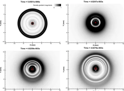
At the first time instances the bubble expands explosively, forming a pressure wave that radiates in a spherical way at all directions (see e.g. Figure 8b, see also Figure 11). It has to be mentioned that this pressure wave reflects on the walls and the free surface, causing a rather complicated pressure field due to the superposition of reflected tension and pressure waves. The bubble expands and reaches a maximum radius and minimum pressure shown below:

- radius 4.3mm at ~1.5ms for case - 1 (ζ~0.006), with minimum bubble pressure 1000Pa - radius 4.5mm at ~1.5ms for case - 2 (ζ~0.009), with minimum bubble pressure 800Pa - radius ~7.2mm at ~2.26ms for case - 3 (ζ~0.014), with minimum bubble pressure 330Pa.

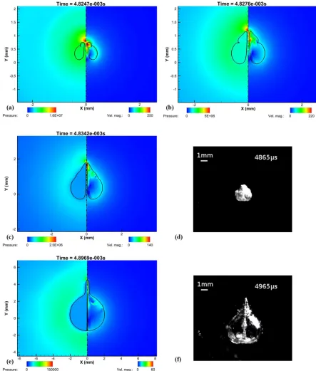
After the maximum bubble size, the bubble starts to collapse. During the collapse, even at the first stages, it is clear that there is a slight bias at the collapse velocity at the bottom of the bubble, i.e. at the bubble interface closest to the bottom of the container. Collapse velocity is slightly higher there (see Figure 9a). This effect is due to the pressure gradient acting on the bubble in the form of hydrostatic pressure. Eventually, this bias acts as a positive feedback mechanism, due to momentum focusing, leading to even higher velocities at the bubble bottom, as the bubble collapses further, see Figure 9c, d. As the bubble reaches closer to its minimum size, a jet forms at the bottom of the bubble, with direction opposite to the pressure gradient, see Figure 9c, d. The relevant photo from the experiment (Figure 9f) shows clearly a deformed, non-spherical bubble, with indications of an internal jet structure. The predictions show that the jet has a radius and velocity as follows:

- radius ~80µm and velocity ~180m/s, for case -1 - radius ~110µm and its velocity ~210m/s, for case - 2

- radius ~110µm and a velocity ~360m/s, for case - 3. Note that this corresponds to a Mach number of ~0.80 for the gaseous phase inside the bubble and ~0.25 for the liquid surrounding the bubble.

the collapse interval where flow dynamics are very fast, running at 1.5.106 frames per second. Also note that the scale is not the same in all the simulation instances, in order to be able to show with full detail the bubble development, especially at collapse.

Figure 7. Comparison between the CFD simulation and the experiment bubble size evolution.

Figure 9. Case 3, ζ=0.014: Bubble collapse. Note the progressively asymmetric velocity and pressure fields. At the last instance the bubble assumes a toroidal shape with the jet on the axis of symmetry. The maximum predicted jet velocity during the collapse is ~360m/s, which corresponds to a Mach number of ~0.80 for the gaseous phase. The magnified insert

in (f) has the same scale as the simulation (e).

Figure 10. Case 3, ζ=0.014: Bubble rebound. Note the jet pierces the bubble forming a toroidal structure. At later stages this forms a protrusion at the bubble surface with a visible needle-like structure inside the bubble, remnant of the jet.

Figure 11. Numerical Schlieren type images, by showing contours of the density gradient. The initial pressure wave due to the bubble expansion is visible, as well as the pressure waves from the jet impact and rebound of the bubble. The red line

shows the bubble interface.

Figure 12. Animation showing the evolution of the bubble. The video is split in half by a vertical line. The left part shows the pressure field and the grey isosurface is a 3D reconstruction of the bubble interface. The right part shows the velocity magnitude and the black continuous line is the bubble interface. Note that due to the large expansion and contraction of the

bubble it is impossible to show with clarity the whole evolution. Thus, at 67µs the camera zooms out and at 4.766ms the camera zooms in closer to the bubble. (Multimedia view).

VI. DISCUSSION

growth stage, as well as at the maximum radius, the bubble size remains closely to spherical for cases 1 to 3, with a maximum deviation from a perfectly spherical shape of ~10µm (or less than 0.2% of the radius). However, during the early stages of the collapse phase there is a slightly higher collapse velocity at the bottom of the bubble, due to existence of the hydrostatic pressure gradient. As the bubble collapses, this slight velocity difference is further amplified due to momentum focusing, that is the concentration of liquid motion to a smaller and smaller region, see 1. Eventually, at an instance close to the rebound, a high velocity jet, with velocity higher than 150m/s, with the exact velocity depending on the case, is generated at the bottom of the bubble with a direction opposite to the pressure gradient. This jet pierces the bubble and then, as the bubble grows, leaves a needle-like trail on the axis of symmetry, while the bubble interface exhibits a conical protrusion, aftermath of the violent jet impact. The predicted behaviour is similar to what is found from experiments 19.

It is of interest to note that even for the small pressure differences encountered in this study, which correspond to a bubble potential energy of less or equal to 10mJ at maximum size, the jet formed at the collapse has a velocity that may exceed 150m/s. Eventually this corresponds to water hammer pressures of at least 2000bar during the impact and even peaking up to 4500bar - such values are comparable with the yield stress of metal alloys as the SS316L 35.

Considering the computational aspects of this work, the following have to be highlighted:

- The whole phenomenon is very sensitive to the accurate resolution of the pressure field. This is especially hindered by the existence of pressure and tension waves. Attention has to be paid to discretization schemes and time stepping, in order to achieve convergence at each time step, good representation of the pressure gradients and accuracy of the interface.

- The computational mesh has to be structured in such a way that it allows accurate resolution of the bubble, both at maximum and minimum bubble sizes. The mesh structuring used in the present work enables high resolution even at very small sizes, due to the O-grid structure.

- Despite the simplistic model of the gaseous phase and the omission of heat transfer effects, the bubble growth/collapse was captured with accuracy, involving the formation of the jet due to hydrostatic pressure gradient.

- To a certain extent, discrepancies from the experiments are to be expected due to the configuration of the container; in the simulations the container corresponds to a cylinder, whereas in reality it is a rectangular domain. This will probably have an effect on the exact wave pattern since the side surface of the cylinder acts as a focusing mirror of pressure waves on the bubble, which lies on the axis of symmetry.

VII. CONCLUSION

ACKNOWLEDGMENTS

The research leading to these results has received funding from the People Programme (IAPP Marie Curie Actions) of the European Union's Seventh Framework Programme FP7/2007-2013/ under REA grant agreement n. 324313. The authors would like to acknowledge the contribution of The Lloyd’s Register Foundation. Lloyd’s Register Foundation helps to protect life and property by supporting engineering-related education, public engagement and the application of research. Also, the authors would like to acknowledge the support of the Swiss National Science Foundation (Grant No. 513234) and the European Space Agency.

Nomenclature

ζ Non-dimensional scaling law (-)

|∇ | Pressure gradient (Pa/m)

ρ Density (kg/m3)

g Acceleration of gravity (m/s2)

Rmax Maximum bubble radius (m)

∞

p Pressure at cavity level (Pa)

nl Tait equation exponent (for liquid) (-)

µ Dynamic viscosity (Pa.s)

u Velocity vector field (m/s)

τ Stress tensor (Pa)

g Acceleration of gravity (m/s2)

f Body/volume forces vector (N/m3)

λ Bulk viscosity coefficient (Pa.s)

a Gas volume fraction

ρ0 Reference density (kg/m3)

c0 Reference speed of sound (m/s)

p0 Reference pressure (Pa)

k Constant of polytropic gas process

(

)

n Polytropic exponent for gas (-)

R Bubble radius (m)

R0 Initial bubble radius (m)

R& Bubble interface velocity (m/s)

R&& Bubble interface acceleration (m/s2)

pv Vapour pressure (Pa)

pg0 Initial gas pressure (Pa)

σ Surface tension (N/m)

∆p Pressure difference (Pa), p∞−pv

References

1. J.-P. Franc and J.-M. Michel, Fundamentals of Cavitation, (2005), Kluwer Academic Publishers.

2. C. E. Brennen, Cavitation and Bubble Dynamics, (1995), Oxford University Press.

4. H. E. Edgerton. David D. Taylor Model Basin and US Office of strategic services, Underwater explosion phenomena, (1943, Unclassified 1947).

5. T. B. Benjamin and A. T. Ellis, The Collapse of Cavitation Bubbles and the Pressures thereby Produced against Solid Boundaries, Philisophical Transactions A 260, 1110 (1966), p. 222-248 DOI: 10.1098/rsta.1966.0046.

6. M. S. Plesset and R. B. Chapman, Collapse of an initially spherical vapor cavity in the

neighborhood of a solid boundary, Journal of Fluid Mechanics 47, (1971), p. 283-290 DOI: 10.1017/S0022112071001058.

7. W. Lauterborn and H. Bolle, Experimental investigations of cavitation-bubble collapse in the neighbourhood of a solid boundary, Journal of Fluid Mechanics 72, 2 (1975), p. 391-399 DOI: 10.1017/S0022112075003448.

8. C. E. Brennen, Fundamentals of Multiphase Flow, (2009), Cambridge University Press. 9. T. G. Leighton, The Acoustic Bubble, (1994), Academic Press.

10. T. M. Mitchell and F. G. Hammitt, Asymmetric Cavitation Bubble Collapse, Journal of

Fluids Engineering 95, 1 (1971), p. 29-37 DOI: 10.1115/1.3446954.

11. J. R. Blake and D. C. Gibson, Cavitation bubbles near boundaries, Annual Review of Fluid

Mechanics 19, (1987), p. 99-123 DOI: 10.1146/annurev.fl.19.010187.000531.

12. M. Tinguely. The effect of pressure gradient on the collapse of cavitation bubbles in normal and reduced gravity, in Faculté des sciences et techniques de l'ingénieur, Laboratoire de

machines hydrauliques (2013), Ecole Polytechnique Federale de Lausanne, Switzerland. p.

120.

13. S. Sauter and C. Schwab, Boundary Element Methods, 1st ed, (2011), Springer-Verlag Berlin Heidelberg.

14. N. Mendez and R. Gonzalez-Cinca, Numerical study of bubble dynamics with the Boundary Element Method, IOP Journal of Physics: Conference Series, International Symposium on

Physical Sciences in Space 327, (2011), p. 9 DOI: 10.1088/1742-6596/327/1/012028.

15. G. L. Chahine, Modeling of Cavitation Dynamics and Interaction with Material, in Advanced

Experimental and Numerical Techniques for Cavitation Erosion Prediction, Kim K-H, et al.,

Editors. 2014, Springer Netherlands. p. 123-161.

16. A. Osterman, M. Dular, and B. Sirok, Numerical simulation of a near-wall bubble collapse in an ultrasonic-field, Journal of Fluid Science and Technology 4, 1 (2009), p. 210-221 DOI: 10.1299/jfst.4.210.

17. N. A. Hawker and Y. Ventikos, Interaction of a strong shockwave with a gas bubble in a liquid medium: a numerical study, Journal of Fluid Mechanics 701, (2012), p. 55-97 DOI: 10.1017/jfm.2012.132.

18. E. Lauer, X. Y. Hu, S. Hickel, and N. A. Adams, Numerical modelling and investigation of symmetric and asymmetric cavitation bubble dynamics, Computers & Fluids 69, (2012), p. 1-19 DOI: 10.1016/j.compfluid.2012.07.020.

19. D. Obreschkow, M. Tinguely, N. Dorsaz, P. Kobel, A. Bosset, and M. Farhat, A Universal Scaling Law for Jets of Collapsing Bubbles, Physical Review Letters 107, 20 (2011), DOI: 10.1103/PhysRevLett.107.204501.

20. D. Obreschkow, M. Tinguely, N. Dorsaz, P. Kobel, A. de Bosset, and M. Farhat, The Quest for the Most Spherical Bubble, Experiments in Fluids 54, 4 (2013), DOI: 10.1007/s00348-013-1503-9.

21. W. Wagner and H.-J. Kretzschmar, International Steam Tables - Properties of Water and Steam based on the Industrial Formulation IAPWS-IF97, 2nd ed, (2008), Springer-Verlag Berlin Heidelberg.

22. M. Farhat, P. Kobel, and D. Obreschkow, Cavitation bubbles in variable gravity: science data. 2014 [cited 2015 27/10/2015]; Available from: http://bubbles.epfl.ch/data.

23. W. Malalasekera and H. Versteeg, An Introduction to Computational Fluid Dynamics: The Finite Volume Method 2nd ed, (2007), Prentice Hall.

24. F. Moukalled, L. Mangani, and M. Darwish, The Finite Volume Method in Computational Fluid Dynamics: An introduction with OpenFOAM and Matlab, Fluid Mechanics and Its Applications, Vol, 113, (2015), Springer International Publishing.

26. G. K. Batchelor, An Introduction to Fluid Dynamics Cambridge Mathematical Library, (2000), Cambridge University Press.

27. J. U. Brackbill, D. B. Kothe, and C. Zemach, A continuum method for modeling surface tension, Journal of Computational Physics 100, (1992), p. 335-354.

28. A. Prosperetti and G. Tryggvason, Computational Methods for Multiphase Flow, (2009), Cambridge University Press.

29. M. J. Ivings, D. M. Causon, and E. F. Toro, On Riemann solvers for compressible liquids,

International Numerical Methods for Fluids 28, (1998), p. 395-418 DOI:

10.1002/(SICI)1097-0363(19980915)28:3<395::AID-FLD718>3.0.CO;2-S.

30. O. Ubbink. Numerical prediction of two fluid systems with sharp interfaces, (1997), Imperial College London.

31. V. Gopala and B. van Wachem, Volume of fluid methods for immiscible-fluid and free-surface flows, Chemical Engineering Journal 141, (2008), p. 204-221 DOI:

10.1016/j.cej.2007.12.035.

32. S. Popinet and S. Zaleski, Bubble collapse near a solid boundary: a numerical study of the influence of viscosity, Journal of Fluid Mechanics 464, (2002), DOI:

10.1017/S002211200200856X.

33. J. F. Thompson, B. K. Soni, and N. P. Weatherill, Handbook of Grid Generation, (1998), CRC Press

34. G. S. Settles, Schlieren and Shadowgraph Techniques: Visualizing Phenomena in Transparent Media, (2001), Springer-Verlag Berlin Heidelberg. 376.