A Blind Comparative Study of Focused Wave Interactions with a Fixed FPSO-like Structure (CCP-WSI Blind Test Series 1)

City, University of London Institutional Repository

Citation

:

Ransley, E., Yan, S. ORCID: 0000-0001-8968-6616, Brown, S. A., Mai, T.,

Graham, D., Ma, Q., Musiedlak, P-H., Engsig-Karup, A. P., Eskilsson, C., Li, Q., Wang, J.,

Xie, Z., Venkatachalam, S., Stoesser, T., Zhuang, Y., Li, Q., Wan, D., Chen, G., Chen, H.,

Qian, L., Ma, Z., Mingham, C., Causon, D., Gatin, I., Jasak, H., Vukcevic, V., Downie, S.,

Higuera, P., Buldakov, E., Stagonas, D., Chen, Q., Zang, J. and Greaves, D. (2019). A Blind

Comparative Study of Focused Wave Interactions with a Fixed FPSO-like Structure

(CCP-WSI Blind Test Series 1). International Journal of Offshore and Polar Engineering, 29(2), pp.

113-127. doi: 10.17736/ijope.2019.jc748

This is the accepted version of the paper.

This version of the publication may differ from the final published

version.

Permanent repository link:

http://openaccess.city.ac.uk/22496/

Link to published version

:

10.17736/ijope.2019.jc748

Copyright and reuse:

City Research Online aims to make research

outputs of City, University of London available to a wider audience.

Copyright and Moral Rights remain with the author(s) and/or copyright

holders. URLs from City Research Online may be freely distributed and

linked to.

City Research Online:

http://openaccess.city.ac.uk/

[email protected]

A blind comparative study of focused wave interactions with a fixed FPSO-like structure

(CCP-WSI Blind Test Series 1)

E. Ransley1_{, S. Yan}2_{, S. Brown}1_{, T. Mai}3_{, D. Graham}1_{, Q. Ma}2_{, P.−H. Musiedlak}1_{, A. P. Engsig−Karup}4_{, C. Eskilsson}5_{, Qian Li}2_, J. Wang2, Z. Xie6, V. Sriram7, T. Stoesser14, Y. Zhuang8, Qi Li8, D. Wan8, G. Chen8, H. Chen9, L. Qian9, Z. Ma9, C. Mingham9, D. Causon9_{, I. Gatin}10_{, H. Jasak}10,11_{, V. Vukˇcevi´c}10_{, S. Downie}12_{, P. Higuera}13_{, E. Buldakov}14_{, D. Stagonas}14_{, Q. Chen}15_{, J. Zang}15_,

D. Greaves1

1: University of Plymouth, UK; 2: City, University of London, UK; 3: National University of Civil Engineering, Vietnam;

4: Technical University of Denmark; 5: Aalborg University, Denmark; 6: CardiffUniversity, UK; 7: Indian Institute of Technology Madras; 8: Shanghai Jiao Tong University, China; 9: Manchester Metropolitan University, UK; 10: University of Zagreb, Croatia; 11: Wikki Ltd, UK;

12: Arup UK; 13: National University of Singapore; 14: University College London, UK; 15: University of Bath, UK

ABSTRACT

Results from Blind Test Series 1, part of the Collaborative Computational Project in Wave Structure Interaction (CCP-WSI), are presented. Partici-pants, with a range of numerical methods, simulate blindly the interaction between a fixed structure and focused waves ranging in steepness and di-rection. Numerical results are compared against corresponding physical data. The predictive capability of each method is assessed based on pres-sure and run-up meapres-surements. In general, all methods perform well in the cases considered, however, there is notable variation in the results (even between similar methods). Recommendations are made for appro-priate considerations and analysis in future comparative studies.

KEY WORDS: Code comparison; numerical validation; CFD; FNPT; PIC; hybrid codes; focused waves; range of steepness; range of incident wave angle; FPSO; run-up and pressure on bow.

INTRODUCTION

Numerical modelling has become an important process in the design of offshore structures and a vast number of tools have been developed as a consequence. The complete range of model fidelity is now available with the trade-offbetween computational efficiency and model complex-ity, i.e. the level of simplification made to the physics being solved, being a key driver when selecting a numerical tool for a particular appli-cation. Despite this, results from the 1st CCP-WSI Focus Group Work-shop demonstrate that there still remain considerable uncertainties in the required level of model fidelity when using numerical methods to simu-late the interaction of waves with offshore structures (CCP-WSI, 2016). Some progress, towards selecting a tool, can be made ahead of time by considering key parameters of the problem, such as the wave and geomet-ric nonlinearity and corresponding dimensionless numbers. However, to promote the routine practical application of numerical tools, particularly

high-fidelity methods, in industrial development processes, greater con-fidence in their applicability needs to be established.

The CCP-WSI Blind Test Workshops have been devised to improve the understanding of this issue and provide information for future de-velopment of numerical modelling standards. These workshops bring together numerical modellers from the wave structure interaction (WSI) community, and assess the numerical codes currently in use, by inviting participants to simulate a series of specific problems, covering a range of relevant complexities, without prior access to the physical measure-ments. The proposed test cases, in each Blind Test Series, are introduced at an introductory event, providing a forum for participants to discuss the cases and the validation process. All required information, to reproduce a set of bespoke physical validation experiments, is then made available in a release event; participants are then invited to submit simulation re-sults for each case before a showcase event, in which the rere-sults from the test and present recommendations are shared with the community.

900 150

153

1200

y _x

z

NOTE: All dimensions in mm MWL

R150

R150

Fig. 1 Structure (M3) dimensions.

CCP-WSI Blind Test Workshops - Series 1

There will be a number of series’ within the CCP-WSI Blind Test Work-shops; Series 1 (the subject of this paper) is held in conjunction with the International Society of Offshore and Polar Engineers (ISOPE) confer-ence, in collaboration with the International Hydrodynamics Committee (IHC); the introductory proposal was presented at the ISOPE conference in San Francisco, USA, on Wednesday 28th June 2017; the release of the Series 1 test cases was made on 12th October 2017, and; the show-case event was held over a series of special sessions at the 2018 ISOPE conference in Sapporo, Japan (10-15th June 2018). For more informa-tion on the CCP-WSI Blind Tests please visit the CCP-WSI website at http://www.ccp-wsi.ac.uk/?q=blind test workshops where supporting material is available including references to complimentary publications, photographs from the experiments and other related resources.

TEST CASES

The CCP-WSI Blind Test Series 1 test cases consist of a fixed, scale-model, floating production storage and offloading (FPSO) vessel (known as M3 (Mai, et al. 2016)) subject to six focused wave events, with a range of steepness,kA =0.13−0.21 and incident angle,α=0◦_,

10◦ & 20◦

, wherekis the wave number associated with the peak period,Tp, of the underlying energy spectrum of the wave andAis the crest amplitude of the crest focused wave assuming linear superposition of the underlying wave components. All cases are free from violent flow features and cor-respond to non-breaking waves with no overturning of the free-surface or greenwater effects. The purpose of these particular test cases is to pro-vide a parametric understanding, based on wave steepness and incident wave angle, of the predictive capabilities of a wide range of numerical WSI codes when assessing critical design factors, such as the pressure and run-up on FPSO hulls, and to evaluate the predictive capability as a function of the code complexity/execution time.

The structure (M3) has vertical sides and each end is semi-circular with the same radius (0.15 m). The full height of the structure is 0.303 m, the length is 1.2 m and the draft is 0.153 m (Figure 1).

The Blind Test Series 1 test cases are split into two parts:

• Part 1 - considers waves of increasing steepness but constant an-gle of incidence, (α=0◦

)

• Part 2 - considers waves with increasing angle of incidence,α, but constant steepness (kA=0.17).

In each experiment, measurements of the pressure on the bow are recorded by an array of pressure transducers (sample frequency, fs,

=1024 Hz). The run-up, at various positions on the hull’s surface, and the free-surface elevation in the vicinity of the structure are recorded by an array of resistive wave gauges (fs=128 Hz).

14.0m 6.0m

4m

Maximum depth 3m

Adjustable floor section Parabolic beach Paddles

Still Water Level (SWL)

2m Working depth, h

4.4m 7.7m

Forward wave gauge 0.3m

y x z

Fig. 2 Schematic of the COAST Laboratory Ocean Basin.

Experimental Set-up

Basin geometry

The experiments were performed in the Coastal, Ocean And Sediment Transport (COAST) Laboratory Ocean Basin (35 m long×15.5 m wide) at the University of Plymouth, UK. The basin has 24 flap-type, force-feedback-controlled wavemakers (hinge depth of 2 m). The water depth at the wavemakers is 4 m and there is a linear slope to the working area where the water depth,h, was set to 2.93 m. At the far end of the basin there is a parabolic absorbing beach (Figure 2).

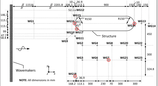
Structure position and wave gauge layout - Part 1

In Part 1 the same wave gauge layout was utilised for both a series of empty tank tests and those with the structure in place (Figure 3).

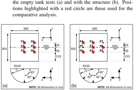
Structure position and wave gauge layout - Part 2

In Part 2, two different arrays of wave gauges were used for the empty tank tests (Figure 4a) and those with the structure present (Figure 4b).

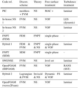
Pressure sensor layout - Part 1

For the cases in Part 1, an array of 6 pressure transducers were positioned on the bow of the FPSO on the centre-line (P1, P2 & P3) and at 45◦

to the port (P4, P5 & P6) side; at the still water level and at depths of±0.05m (Figure 5a).

Pressure sensor layout - Part 2

In Part 2, an array of 9 pressure transducers were positioned on the bow of the FPSO on the centre-line (P1, P2 & P3) and at 45◦

to the port (P7, P8 & P9) and starboard (P4, P5 & P6) sides; at the still water level and at depths of±0.05m (Figure 5b).

Wavemakers

Structure

WG1

WG12 WG15 WG16

WG17 WG10

WG11

WG9 _{WG2 WG4 WG8 WG20 WG22}

WG3 WG6 WG7 WG21 WG23

WG18

WG24 WG13

WG14

150 140

150 10

R150 R150

900

300 450

324.8

300 300

300 230 70

45° 45° 113.1

113.1 36.9 36.9 10

52.1 106.1

y x z

NOTE: All dimensions in mm 146.7

168.2 113.1

113.1 99 47.7 58.4

2201.8 11516

Wavemakers WG1 WG12 WG10 WG11 WG9 WG7 WG13 WG14 R150 R150 62.1 680 670 300 468.5 150 150 150 150 900 109.6 757 12391 310 168.2 88.2 88.2 116.6 69.5 47.1 58.4 45° WG5 WG8 54.4 54.4 121.4 46.4 103.7 WG2 295 WG3 WG4 WG15 WG16 WG17 WG6 α y x z

NOTE: All dimensions in mm

Wavemakers Structure WG1 WG12 WG15 WG16 WG17 WG10 WG11 WG9 WG18 WG7 WG24 WG13 WG14 150 140 150 10 R150 R150 300 300 290 300 670 680 45° 45° 113.1 36.9 10 52.1 106.1 146.7 113.1 113.1 99 47.7 58.4 2201.8

11516 200 200 200

WG19 WG20 WG21 WG22 WG23 45° ₁₅₀ 10 WG5 WG8 α y x z

NOTE: All dimensions in mm

(a)

(b)

Fig. 4 Structure positioning and wave gauge layout for Part 2, for the empty tank tests (a) and with the structure (b). Posi-tions highlighted with a red circle are those used for the comparative analysis. 300 R150 MWL 50 50 303 45° 45° 153 300 R150 MWL 50 50 303 45° 45° 45° 153

P4 P1 P7

P5 P2 P8

P6 P3 P9

(a) (b) P1 P4 P5 P3 P6 y z x y x z y z x y x z

NOTE: All dimensions in mm NOTE: All dimensions in mm P2

Fig. 5 Pressure probe layout on the bow of the FPSO for Part 1 (a), and; for Part 2 (b). Positions highlighted with a red circle are those used for the comparative analysis.

Test Program

For each test case, the incident waves were generated in the COAST Lab-oratory Ocean Basin (Figure 1) using the EDL paddle control software. The software is designed to reproduce the desired free-surface elevation by applying various corrections to account for the change in water depth in front of the wave paddles and the nonlinear propagation of the wave fronts. In this case, each wave was create using linear superposition of 244 wave fronts with frequencies evenly spaced between 0.101563 Hz and 2 Hz. All waves in this study are non-breaking and trough focused, i.e. each of the contributing wave components has a phase ofπat a the-oretical focus location,x0. The amplitudes of the frequency components

are derived by applying the NewWave theory (Tromans et al. 1991) to a JONSWAP spectrum with the parameters given in Table 1. Each wave front is then transformed back to the position of the wave paddles by the control software andx0is iteratively adjusted (as described by Hann et al. 2015) to pragmatically ensure focusing, i.e. a symmetric event, at the position coincident with the bow of the FPSO.

Wave parameters - Part 1

In Part 1, the three waves are all generated with an incident wave angle,

α = 0◦

. Two wave cases (11BT1 & 12BT1) differ only byHs and so 12BT1 is essentially a steeper version of 11BT1 with the same relative frequency contributions; two cases (12BT1 & 13BT1) differ only by peak frequency,Tp, so 13BT1 is essentially a steeper version of 12BT1 with the sameHs(Table 1).

Wave parameters - Part 2

In Part 2, all three waves have the same steepness (kA = 0.17). The waves differ only by incident angle,α(Table 1).

Table 1 Wave conditions used in the CCP-WSI Blind Test Series 1

Case kA α Hs Tp

Part 1

11BT1 0.13 0◦

0.077 m 1.456 s

12BT1 0.18 0◦

0.103 m 1.456 s

13BT1 0.21 0◦

0.103 m 1.362 s

Part 2

21BT1 0.17 0◦

0.103 m 1.456 s

22BT1 0.17 10◦

0.103 m 1.456 s

23BT1 0.17 20◦

0.103 m 1.456 s

Released Data

The CCP-WSI Blind Test Series 1 is a blind validation of numerical WSI codes. Consequently the only physical measurement data released to participants prior to submission, were surface elevation data from the wave gauges in the empty tank tests (see Figures 3 & 4a for the wave gauge positions). This data is deemed sufficient to reproduce the incident waves in each of the cases including the FPSO, for which the same wave-maker signals were used. The remaining physical measurements were not released until after all participants had submitted their final results and it is these ‘blind’ results that are reported in this paper.

Physical Measurement Errors and Experimental Limitations

As the predictive capability of the numerical submissions is judged on their ability to reproduce the physical results, it is absolutely necessary to also consider the errors present in the physical measurements. This is particularly pertinent in the cases presented here as, not only are the numerical results compared against the physical measurements but, all of the numerical simulations are initiated (in some way) using values derived from the physical measurements in the empty tank tests.

a relative standard deviation of 2.6% is observed. This is considered to be the maximum level of random error in the physical surface elevation measurements, in this test, and thus a maximum confidence interval of

±7.8% in the run-up has been assumed, i.e. 99.7% of data values can be considered to be within three standard deviations.

Confidence in the pressure measurements is significantly lower. Due to the intermittent wetting of the pressure probes, some of the pressure records are effected by thermal shock. This results in nonphysical fluctu-ations in the pressure measurements at frequencies similar to those of the physical signal. Consequently, traditional filtering, based on frequency-space methods, cannot remove this effect and so a bespoke ‘thermal shock filter’ has been designed to remove the unwanted signal. This new method is still under development and, as yet, is still not capable of distinguishing the smallest peaks in pressure from the background noise and has, therefore, resulted in these being removed from the filtered data. However, once applied, the pressure measurements from three experi-ments demonstrate excellent repeatability with the variation between test being lower than the noise in the signal (≈0.005 Pa).

Systematic errors in the physical measurements are considered to be negligible in the cases considered here. The wavelength of the waves is sufficient that minor inaccuracies in the probe positions (on the order of 10 mm) are not important. The triggering of the various data acquisition systems is a potential source of issues. In these cases, because the numer-ical codes use the surface elevation measurements in the empty tank tests to initialise their models, the only issue is the triggering of the pressure probe measurements relative to the surface elevation measurements. The delay in the triggering is well understood in the COAST Laboratory and has been accounted for precisely in the results reported here.

NUMERICAL METHODS

Participating Codes

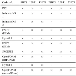
The CCP-WSI Blind Test Series 1 involved 33 participants, from 15 aca-demic institutions, and industry collaborators, from 8 different countries. There are submissions using 10 different numerical codes/methods rang-ing from fully nonlinear potential theory (FNPT) to Navier-Stokes (NS) solvers; including hybrid (coupled) methods, partially particle methods, finite element methods, finite volume methods, both open-source and in-house codes and both low-order accurate and high-order accurate codes. Each method is described below and the main characteristics of each im-plementation are summarised in Table 2.

Particle-In-Cell (PIC) method

This solver utilises the hybrid Eulerian-Lagrangian Particle-In-Cell (PIC) method to solve the incompressible NS equations for single-phase free-surface flows, incorporating a Cartesian cut cell-based, two-way, strong coupling algorithm for fluid-structure interaction (Chen et al., 2018; Chen & Zang, 2018). In this method, the Lagrangian particles are used to solve the nonlinear advection terms and track the free-surface, while the Eulerian grid is employed for solving the non-advection terms with robustness and efficiency. The focused wave is generated using a piston-type wave paddle whose velocity and position are determined according to the NewWave theory and first-order wavemaker theory. Wave absorp-tion is achieved through the relaxaabsorp-tion zone approach. The computa-tional domain is 24 m long, 3.025 m wide and 3.5 m high and is dis-cretised by a uniform grid of size 0.025 m with eight particles being seeded in each cell accommodating the fluid area (which results in ap-proximately 16 million grid cells and 105 million particles). The solution in time is first-order accurate and the time step is controlled by a Courant number of 0.5. No turbulence modelling is included, i.e. laminar flow is assumed. Computations are performed using 72 cores (6 Intel Xeon Gold 6126 CPUs) of an in-house high-performance computing (HPC) facility.

Table 2 Summary of numerical methods used by participants

Code ref. Discret. scheme

Theory Free-surface treatment

Turbulence treatment

PIC meshless

+FVM

NS MAC+ laminar

In-house NS 1

FVM NS VOF LES

(dynamic)

In-house NS 2

FVM NS VOF laminar

FNPT (FEM)

FEM FNPT single-phase

-Hybrid 1 FEM &

FVM

FNPT & NS

single-phase & VOF

laminar

FNPT (SEM)

SEM FNPT single-phase

-SWENSE FVM NS level set laminar

OpenFOAM (IHFOAM)

FVM NS VOF RANS

(SST)

Hybrid 2 Lagrangian

& FVM

Inviscid & NS

Dynamic FS & VOF

laminar

OpenFOAM (waves2Foam)

FVM NS VOF laminar

In-house NS solver 1

This method utilises a two-phase flow model to solve the filtered NS equations using the finite volume method (FVM) and the high-resolution volume of fluid (VOF) scheme, CICSAM (compressive interface captur-ing scheme for arbitrary meshes), on a staggered Cartesian grid. The partial cell treatment in 3D is used to allow for complex geometries in the domain (Xie, 2015). The advection terms are discretised by a high-resolution scheme which combines the high order accuracy with mono-tonicity (Xie, 2012). The gradients in pressure and diffusion terms are obtained by central difference schemes. An expression-based boundary condition, based on the superposition of linear wave components derived from the empty tank tests, is used to define the time history of wave elevations and velocities at the inlet. For wave absoption, a radiation outlet boundary condition is used. In this study, the computational do-main is 6 m long, 3 m wide and 3.3 m high; it has a uniform mesh with size 0.01875 m in the horizontal and 0.01 m in the vertical (total number of mesh cells≈16.4 million). The SIMPLE algorithm for the pressure-velocity coupling is employed and a backward finite difference discreti-sation is used for the time derivative (Xie et al., 2018). Large-eddy simulation is employed for the turbulence modelling with the dynamic Smagorinsky model. The computation of the test cases was performed using 512×2.6 GHz cores of an in-house HPC cluster.

In-house NS solver 2

absorp-tion is achieved via an artificial viscous term in the momentum equaabsorp-tion, i.e. a sponge layer. In this study, the computational domain is 23 m long and 4 m wide. The mesh is unstructured with a free-surface refinement layer consisting of>40 cells over the wave height and>80 cells over the characteristic wavelength; further refinement is present around the FPSO (≈5.7 million cells in total). A fixed time step ofdt =0.01 s is used throughout. No turbulence modelling is included, i.e. laminar flow is assumed. The computation of the test cases was performed using 64×

2.8 GHz cores (IBM NeXtScale nx360 m4 model) (Li et al., 2018a).

FNPT solver (using FEM)

In QALE-FEM (Quasi Arbitrary Lagrangian-Eulerian Finite Element Method) the flow is governed by the FNPT model where a boundary value problem for velocity potential is solved using the FEM. A simi-lar boundary value problem is solved to find the time derivative of the velocity potential in the Bernoulli equation, which is used to find the force acting on floating structures. The fully nonlinear free surface con-ditions are written in arbitrary Lagrangian-Eulerian forms (Ma & Yan, 2006; Yan & Ma 2010). Wave generation and absorption is achieved us-ing self-adaptive wavemakers. In this study, as the incident waves are uni-directional, a quasi-2D domain is combined with a 3D domain us-ing a weak zonal couplus-ing. The 2D domain has the same dimensions as the experimental wave basin (Figure 2) but is very coarse in the direc-tion normal to the wave propagadirec-tion, i.e. 5 cells wide, whereas the 3D domain consists of a cylindrical domain (radius 3.5 m) centered on the FPSO. The 3D domain has a graded mesh with a characteristic mesh size of 0.03 m near the free-surface and 0.02 m on the surface of the FPSO (≈3.45 million mesh cells total). The time discretisation scheme is a 2nd order finite difference scheme and the time step is fixed at 128 Hz to be consistent with the physical data. The computation of the test cases was performed using 4×2.9 GHz cores (Xie et al., 2018).

Hybrid method 1

The hybrid FNPT-NS solver, qaleFOAM, combines QALE-FEM (see above) and OpenFOAM’s multiphase NS solver interDyMFoam using a domain decomposition method and a coupling boundary (Li et al. 2018b). Wave generation and absorption is achieved using self-adaptive wavemakers on the inlet and outlet of the the FNPT region which covers the whole computational domain with the same size of the experimental wave basin (Figure 2). The mesh in the FNPT domain has a characteristic size of 0.04 m. The NS domain is confined to a small region (5.4 m×3×

3.53 m) surrounding the structure and is bounded by the coupling bound-ary upon which the velocity, pressure and wave elevation values for the NS solver are provided by the QALE-FEM. The mesh in the NS region is graded with approximately 50 cells over the maximum wave height and 180 cells per peak wavelength in the free-surface region and a char-acteristic cell size of 0.005 m on the FPSO surface (≈1.96 million mesh cells total). The time stepping is first order accurate (Implicit Euler) and dynamic, based on a Courant-Friedrichs-Lewy (CFL) condition of 0.5. No turbulence modelling is included, i.e. laminar flow is assumed. The computation of the test cases was performed using 8×2.6 GHz cores.

FNPT solver (using spectral element method (SEM))

This method is based on a stabilised spectral element method (SEM) us-ing a Galerkin spatial discretization and an explicit Runge-Kutta method for the temporal integration of an Eulerian formulation of the fully nonlinear potential flow (FNPF) equations (Engsig-Karup et al., 2016; Engsig-Karup & Eskilsson, 2018). The FNPF-SEM solver is high-order accurate and represents the solution variables on an unstructured mesh through the globally continuous piece-wise polynomial basis functions. Wave generation and wave absorption is done using a standard embedded penalty method (Engsig-Karup et al., 2013). Incident waves are

gener-ated using superposition of first-order linear wave components derived from the empty tank data using a discrete Fourier transform. The com-putation domain is 12 m long and 8 m wide. The grid is relatively coarse consisting of two vertical layers and a total number of prism elements on the order of 10,000 (≈500,000 nodes (degrees of freedom) in the fluid volume discretisation). The FPSO is captured to high accuracy using curvilinear faces in the top layer that also account for the curvilinear free surface representation. The time-stepping is based on a fourth-order ex-plicit Runge-Kutta method with time step sizes ofdt = 0.025 s in all simulations. The computations of the test cases were performed in MAT-LAB R2017a and executed sequentially (i.e. no code parallelisation).

Spectral wave explicit Navier-Stokes equations (SWENSE) solver

The Naval Hydro Pack is a specialised software library based on the foam-extend, collocated finite volume computational fluid dynamics (CFD) software. In this method the spectral wave explicit Navier-Stokes equations (SWENSE) method is used to couple the incident wave field and the CFD solution (Vukˆcevi´c et al., 2016). A two-phase flow model is used with the level set method for interface capturing; the ghost fluid method is used to take into account the discontinuities in fields across the interface (Vukˆcevi´c et al., 2017). Waves are generated using implicit relaxation zones (Jasak et al., 2015) which are positioned along the edge of the computational domain which, in the cases studied here, is 20.7 m long, 7 m wide and 3.53 m high. The mesh is graded towards the struc-ture, with a resolution corresponding to∆x=0.01 m,∆y=0.02 m and

∆z = 0.005 m in the vicinity of the hull surface, resulting in approxi-mately 4.1 million cells in total. The time-step is controlled to maintain a CFL number below 1, resulting in time-steps ranging from 0.005 to 0.015 s. An implicit second order backward time marching scheme is used. No turbulence models are used, instead laminar flow is simulated. Simulations are performed using 21 cores of the Intel Xeon Processor E5-2637 v3 (15M Cache, 3.50 GHz) (Gatin et al., 2018).

Open-source NS solver (OpenFOAM using IHFOAM)

This method utilises OpenFOAM (ESI version 1706), an open-source CFD software based on the finite volume discretisation. The standard interFoam solver is used to solve the RANS equations for two, incom-pressible, isothermal and immiscible fluids using a VOF interface cap-turing scheme. The IHFOAM toolbox provides the functionality of wave generation and active wave absorption (Higuera et al., 2013). A member function has been added to generate phase-focused waves based on sec-ond order irregular wave theory and wave components derived from the given wave conditions and spectra. The computational domain is 10 m long, 4 m wide and 3.43 m high. The spatial discretisation takes the form of an unstructured mesh, consisting mostly of hexes, with a typical reso-lution of 0.0085 m in the region of the free surface, and 0.00425 m around the structure. The total number of mesh cells used in each case is approx-imately 3.1 million. The time stepping is first order accurate (Implicit Euler) and dynamic, based on a CFL condition of 0.35. No turbulence modelling is included, i.e. laminar flow is assumed. The computations were performed using 48×1.7 GHz cores of an in-house HPC facility.

Hybrid method 2

used as inlet boundary conditions in the RANS simulations. To ensure the target waves are generated regardless of any reflected waves reach-ing the boundary a new one-way couplreach-ing technique has been developed (Higuera et al., 2018). Incident waves are also absorbed at the opposite boundary using the same technique coupled with an enhanced version of the active wave absorption presented in Higuera et al. (2013). The spatial discretisation in the Lagrangian model is 251×16 and the time step is 0.005 s. The CFD mesh is 15 m×1.7 m×3.16 m and unstruc-tured, but hexahedral-cell dominant, with a maximum cell resolution of 0.01 m, adjacent to the FPSO (total number of cells≈46.5 million). The time stepping is first order accurate (Implicit Euler) and dynamic, based on a CFL condition of 0.15. No turbulence modelling is included. The computation of the test cases was performed using 120×2.6 GHz cores.

Open-source NS solver (OpenFOAM using waves2Foam)

This method utilises OpenFOAM (Foundation version 4.1), an open-source CFD software based on the finite volume discretisation (Brown et al. 2018). A modified version of the standard interFoam solver is used to solve the RANS equations for two incompressible, isothermal and immiscible fluids using a VOF interface capturing scheme. The waves2Foam toolbox (Jacobsen et al., 2012) provides wave generation through a linear superposition of first order wave components (hierar-chically selected based on a fast Fourier transform (FFT) of the phys-ical empty tank data (Musiedlak et al. 2017)). Wave absorption is achieved using the relaxation zone functionality provided as part of the waves2Foam toolbox. The computational domain is 14 m long, 6 m wide and 4 m high. The spatial discretisation takes the form of an unstructured mesh, consisting mostly of hexes, with a typical resolution of 0.025 m in the region of the free surface, and 0.00625 m around the structure. The total number of mesh cells used in each case is approximately 1.9 million. The time stepping is first order accurate (Implicit Euler) and dynamic, based on a CFL condition of 0.25. No turbulence modelling is included, i.e. laminar flow is assumed. The computation of the test cases was performed using 16×2.6 GHz cores of an in-house HPC facility.

Submissions

Participation in the CCP-WSI Blind Test Series 1 is purely voluntary and so, as a consequence, some participants only managed to complete a selection of the test cases. Table 3 summarises the test cases that were submitted for each code/method (where an ‘×’ signifies a submission).

RESULTS & DISCUSSION

Time Series Analysis

As highlighted in Figures 3, 4 and 5, participants were requested, in each of the six cases, to submit times series data for five different surface el-evation probe positions and six different pressure probe positions. As a result, a huge data set is available for the comparative study. However, the processing of all the data has been deemed impractical and so, after reviewing all of the data qualitatively, a representative sample has been selected and reported here. In general, the same trends are observed for all of the measurements and so the run-up on the bow (probe WG16) and the pressure on the bow, at the still water level (probe P2), have been considered as being arguably most relevant to design engineers etc.

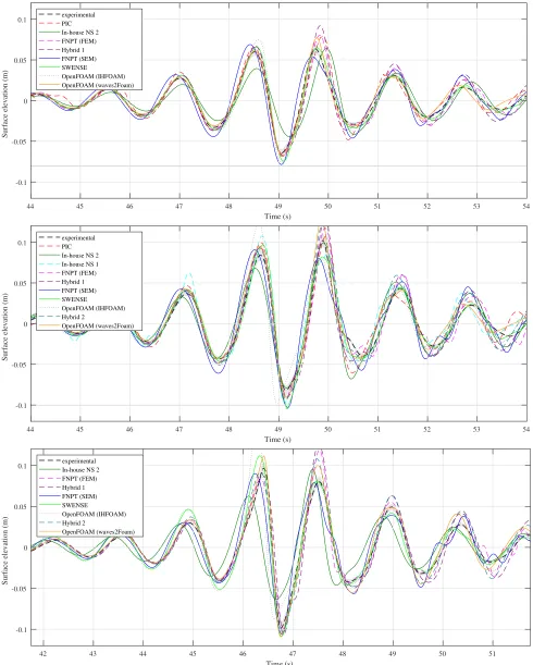
Run-up at the bow

Figure 6 shows the physical measurements (including the 99.7% confi-dence interval), as well as all of the numerical submissions, for run-up on the bow of the FPSO, for all three cases in Part 1, i.e. for increas-ingly steep waves with zero incident wave angle. The results show that, for the range of wave steepness considered, all of the numerical methods

Table 3 Submitted test cases for each of the participating codes

Code ref. 11BT1 12BT1 13BT1 21BT1 22BT1 23BT1

PIC × × - × × ×

In-house NS 1

- × - - -

-In-house NS 2

× × × - -

-FNPT (FEM)

× × × × × ×

Hybrid 1 × × × - -

-FNPT (SEM)

× × × × × ×

SWENSE × × × × × ×

OpenFOAM (IHFOAM)

× × × - -

-Hybrid 2 - × × - -

-OpenFOAM (waves2Foam)

× × × × × ×

are able to predict the general behaviour well, particularly the phasing of the wave event, and that there is no obvious trend between the predictive capability of the methods and their underlying complexity, i.e. for the (non-breaking) cases consider here, there appears to be no clear advan-tage in using high fidelity methods over FNPT. There is, however, quite a range in the predicted amplitudes of the crests and troughs with a distinct tendency for the numerical simulations to over-predict, particularly the crest immediately following the main trough. Qualitatively, it is possible that these discrepancies increase with wave steepness, i.e there appears to be significant difficultly in reproducing the crest immediately before the main trough in the steepest case (Figure 6c). However, quantitative anal-ysis is required to provide conclusive evidence of this (and there is still no evidence that higher-fidelity models perform better, even for the steepest case considered here). Lastly, a few seconds after the main trough, the predictive capability of the numerical models is greatly reduced and the variation in the predictions is large. However, this observation is almost certainly due to the differing treatment of reflected waves in each of the numerical methods; as the reflective characteristics of the physical beach were not released, participants are not expected to be able to reproduce this part of the time series nor is it used to judge the submissions.

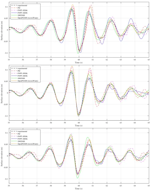
Figure 7 shows the run-up on the front of the FPSO, for all three cases in Part 2, i.e. for a fixed wave steepness and increasing incident wave angle. The same observations can be made as above: all numerical meth-ods perform reasonably well with well-reproduced phasing in each of the cases; there is some variation in the amplitudes with a tendency for over-prediction, but again; there is no obvious advantage in using high-fidelity methods for the cases considered in this study. Lastly, in the cases con-sidered here, when considering the run-up on the bow of the FPSO, there does not appear to be any trend between the predictive capability of the numerical models and the incident wave angle.

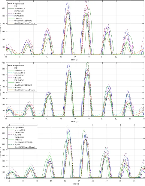
Pressure on the bow

repro-44 45 46 47 48 49 50 51 52 53 54 Time (s)

-0.1 -0.05 0 0.05 0.1

Surface elevation (m)

experimental PIC In-house NS 2 FNPT (FEM) Hybrid 1 FNPT (SEM) SWENSE

OpenFOAM (IHFOAM) OpenFOAM (waves2Foam)

44 45 46 47 48 49 50 51 52 53 54

Time (s) -0.1

-0.05 0 0.05 0.1

Surface elevation (m)

experimental PIC In-house NS 2 In-house NS 1 FNPT (FEM) Hybrid 1 FNPT (SEM) SWENSE

OpenFOAM (IHFOAM) Hybrid 2

OpenFOAM (waves2Foam)

42 43 44 45 46 47 48 49 50 51

Time (s) -0.1

-0.05 0 0.05 0.1

Surface elevation (m)

experimental In-house NS 2 FNPT (FEM) Hybrid 1 FNPT (SEM) SWENSE

OpenFOAM (IHFOAM) Hybrid 2

OpenFOAM (waves2Foam)

55 56 57 58 59 60 61 62 63 64 65 Time (s)

-0.1 -0.05 0 0.05 0.1

Surface elevation (m)

experimental PIC FNPT (FEM) FNPT (SEM) SWENSE

OpenFOAM (waves2Foam)

55 56 57 58 59 60 61 62 63 64 65

Time (s) -0.1

-0.05 0 0.05 0.1

Surface elevation (m)

experimental PIC FNPT (FEM) FNPT (SEM) SWENSE

OpenFOAM (waves2Foam)

55 56 57 58 59 60 61 62 63 64 65

Time (s) -0.1

-0.05 0 0.05 0.1

Surface elevation (m)

experimental PIC FNPT (FEM) FNPT (SEM) SWENSE

OpenFOAM (waves2Foam)

Fig. 7 Run-up on the bow of the FPSO for cases in Part 2 (Probe WG16), i.e. increasing angle of incidence from (a) 21BT1 (α=0◦

) to (b) 22BT1 (α=10◦

) to (c) 23BT1 (α=20◦

44 45 46 47 48 49 50 51 52 53 54 Time (s)

0 100 200 300 400 500 600

Pressure (Pa)

experimental PIC In-house NS 2 FNPT (FEM) Hybrid 1 FNPT (SEM) SWENSE

OpenFOAM (IHFOAM) OpenFOAM (waves2Foam)

44 45 46 47 48 49 50 51 52 53 54

Time (s) 0

100 200 300 400 500 600 700 800 900

Pressure (Pa)

experimental PIC In-house NS 2 In-house NS 1 FNPT (FEM) Hybrid 1 FNPT (SEM) SWENSE

OpenFOAM (IHFOAM) Hybrid 2

OpenFOAM (waves2Foam)

42 43 44 45 46 47 48 49 50 51

Time (s)

0 100 200 300 400 500 600 700 800 900

Pressure (Pa)

experimental In-house NS 2 FNPT (FEM) Hybrid 1 FNPT (SEM) SWENSE

OpenFOAM (IHFOAM) Hybrid 2

OpenFOAM (waves2Foam)

55 56 57 58 59 60 61 62 63 64 65 Time (s)

0 100 200 300 400 500 600 700 800

Pressure (Pa)

experimental PIC FNPT (FEM) FNPT (SEM) SWENSE

OpenFOAM (waves2Foam)

55 56 57 58 59 60 61 62 63 64 65

Time (s) 0

100 200 300 400 500 600 700 800

Pressure (Pa)

experimental PIC FNPT (FEM) FNPT (SEM) SWENSE

OpenFOAM (waves2Foam)

55 56 57 58 59 60 61 62 63 64 65

Time (s) 0

100 200 300 400 500 600 700

Pressure (Pa)

experimental PIC FNPT (FEM) FNPT (SEM) SWENSE

OpenFOAM (waves2Foam)

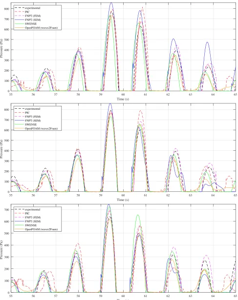
Fig. 9 Pressure on the bow of the FPSO, at the still water level (probe P2), for cases in Part 2, i.e. increasing angle of incidence from (a) 21BT1 (α = 0◦

) to (b) 22BT1 (α = 10◦

) to (c) 23BT1 (α = 20◦

duce the pressure reasonably well, there appears to be a greater spread in the predicted phasing compared to the surface elevation, and there is considerable variation in the predicted amplitude of the peaks (again typ-ically over-estimates). Again, the predictive capability of the numerical models is greatly reduced a few seconds after the main peaks but this can again be attributed to the variation in the treatment of reflected waves, but, there is again no clear relationship between the predictive capabil-ity of the models and either the incident wave angle or the wave steep-ness. However, in the steepest case (Figure 8c), the predictions of the crest immediately before the main trough do appear to show the greatest variability. There is, again, no obvious benefit in using higher-fidelity methods for the (non-violent) wave cases considered here. Lastly, it has been noticed that there is a large variation in the prediction of hydrostatic pressure between the numerical methods.

Quantitative Analysis

Comparisons of time series’ are valuable, in that all the data are present without manipulation or the introduction of bias (from analysis methods that favour one data set over another). However, only qualitative compar-isons can be drawn directly and with so many participants and with mul-tiple cases to analyse, it is not possible to ascertain conclusive evidence of any parametric trends in the data. Therefore, a series of strategies are investigated here in order to quantify the predictive capability of the nu-merical methods into a limited number of discrete values and allow for more simplified visualisation of any trends in the data.

Root Mean Squared (RMS) error

A root mean squared (RMS) error calculation is perhaps the simplest es-timation of the ‘error’ associated with any particular reproduction of a time series. An RMS error, in these cases, is defined as the square root of the arithmetic mean of the squares of the differences between the repro-duction (numerical submission) and the original (the physical data). This then returns a single number representation of the predictive capability of the numerical method. However, in the general case, the time vector of the original time series does not match that of the reproduction (par-ticularly when the numerical method uses adaptive time-stepping) and so some form of interpolation is typically required before an RMS can be calculated, adding an additional layer of uncertainty around the predic-tion. Furthermore, although convenient for analysis of many multivariant data sets, reducing the measure of predictive capability to a single num-ber removes large amounts of (potentially valuable) information about the reproduction and can lead to a significant bias in the results. For ex-ample, in an otherwise perfect reproduction of the original time series, a small phase shift in the prediction can result in a very large RMS error, particularly in cases with steep gradients in the measured quantity, and so this form of analysis favours those methods that predict the phases well. Therefore, in cases in which the timings of events are less critical (compared to the amplitude), an RMS is not an appropriate measure of the quality of the prediction. Despite this, the RMS in the predicted run-up on the bow of the FPSO has been calculated (for a window of time starting 5 seconds before the main trough in the physical data and end-ing 5 seconds after) and plotted against both the waves steepness (Figure 10) and the incident wave angle (Figure 11). Also plotted is the RMS error in each submission against the CPU effort for each simulation (Fig-ure 12). CPU effort has been estimated as the execution time, multiplied by the number of cores used, divided by the simulated time (it should be noted that this estimation does not account for the different hardware used by each of the participants, nor were participants asked to minimise the CPU effort in their submissions). In each figure, the data has been colour-coded according to the underlying theory/method, i.e. red sym-bols symbolise NS solvers, blue symbolises FNPT solvers, cyan is used for the hybrid methods and the PIC method is coloured in magenta.

0.1 0.15 0.2 0.25

Wave steepness (kA) 0

0.005 0.01 0.015 0.02 0.025 0.03

RMS (m)

PIC In-house NS 2 In-house NS 1 FNPT (FEM) Hybrid 1 FNPT (SEM) SWENSE OpenFOAM (IHFOAM) Hybrid 2

OpenFOAM (waves2Foam)

Fig. 10 RMS vs. wave steepness for numerical predictions of run-up on the bow of the FPSO (WG16), in Part 1.

-5 0 5 10 15 20 25

Incident Wave Angle (degrees)

0 0.005

0.01 0.015 0.02 0.025 0.03

RMS (m)

PIC FNPT (FEM) FNPT (SEM) SWENSE

OpenFOAM (waves2Foam)

Fig. 11 RMS vs. incident wave angle for numerical predictions of run-up on the bow of the FPSO (WG16), in Part 2.

103 104 105 106 107

CPU time (s) per second of simulation 0

0.005 0.01 0.015 0.02 0.025 0.03

RMS (m)

PIC In-house NS 2 In-house NS 1 FNPT (FEM) Hybrid 1 FNPT (SEM) SWENSE

OpenFOAM (IHFOAM) Hybrid 2

OpenFOAM (waves2Foam)

There is significant scatter in the RMS values calculated and so low confidence in any trends observed. There appears to be a reduction in the RMS as the incident wave angle increases and potentially an increase in the RMS as the wave steepness increase. However, the amplitude of the run-up on the centre of the bow is also seen to reduce with incident wave angle and the most significant increase in RMS occurs between cases 11BT1 and 12BT1 (0.13<kA<0.18), i.e. a rise in steepness due to an increase in wave amplitude. Therefore, it is suspected that any increase in RMS is likely due to an increase in wave amplitude and that steepness and direction does not have a dominant effect in these cases. Further-more, as observed in the qualitative analysis of the time series data, the FNPT methods have performed equally as well as the high fidelity meth-ods; it could be argued that the NS solvers achieve the lowest RMS values but NS solvers are also responsible for the greatest RMS values high-lighting a potential concern over the apparently high variability in the results produced when solving fundamentally the same set of equations. Figure 12 shows, perhaps, the most conclusive result; FNPT solvers are significantly quicker at solving these cases than NS solvers without a sig-nificant decrease in the RMS error. The FEM-based FNPT method is at least 1.5 orders of magnitude faster than the quickest NS code and has comparable predictive capability in these cases. The FNPT method based on SEM is significantly slower in comparison and has a slightly greater RMS, however, this is a relatively new implementation of the method and with further refinement it is anticipated that this method will be compet-itive with the more established FNPT (FEM) method. Again, NS solvers display both the lowest and highest RMS values and the spread in CPU effort for NS solvers is also very large. It is suspected that these variations are due mostly to the wide range of mesh/domain designs, wave genera-tion/absorption strategies and CPU resources used. This highlights that, either ‘best practice’ procedures for these applications are not known or participants are not adhering strictly to them. Finally, the two hybrid methods, although relatively new implementations, do not display any benefit over the other methods, i.e. in the cases reported here, there is no saving of CPU effort over NS-only solvers nor is there any improvement in the prediction over FNPT methods.

Multi-value assessment methods

As mentioned above, although convenient for identifying trends across multiple cases, the RMS error may not be an appropriate measure of the predictive capability of a code, particularly in some cases where signif-icant bias is introduced, i.e. cases with high gradients and small phase discrepancies. Furthermore, as a single-value representation of accuracy, the RMS does not allow for differentiation between the errors associated with individual variables in multivariant data sets, i.e. amplitude, phase, frequency-content etc. In fact it is not possible for a single-value assess-ment method to provide this information directly; the method must pro-duce at least the same number of values as the variables under scrutiny.

A number of multi-value assessment methods have been considered here: The cross-correlation can be used to find the similarity between two time series as a function a time shift (phase shift) of one series rel-ative to the other; the ‘lag’ associated with the maximum similarity and the value of the maximum similarity then gives a two-value estimate of the reproduction incorporating a measure of the phase prediction and the amplitude prediction without introducing a bias due to a phase discrep-ancy (this is essentially equivalent to shifting the predicted time series in time to minimise the RMS error and then recording the time shift and the minmised RMS. This idea is also equivalent to performing the lin-ear least-squares approach from regression analysis which minimises the sum of the squares of the differences between the physical value and the model data points). This method, however, does not provide any infor-mation regarding the frequency content in the reproduction and a poor similarity could be due to either a frequency content discrepancy or an

amplitude discrepancy. An alternative assessment method could be to use a dynamic time warping (DTW) algorithm which determines a mea-sure of similarity independent of nonlinear variations in the time dimen-sion, i.e. unlike the cross-correlation, the sequence alignment method, or ‘warping’, is non-uniform and nonlinear. DTW returns a ‘distance-like’ quantity, know as the Euclidean distance, describing the ‘distance’ be-tween the two signals in the time dimension which incorporates discrep-ancies in both phase and frequency content. A two-value assessment can then be completed by performing an RMS analysis of the target and the warped time series’ giving an error estimate in the amplitude that is ar-guably independent of any inaccuracy in the phase or frequency content. Frequency domain analysis methods, such as Fourier transforms, offer a multi-valued assessment method consisting of the power (amplitude) as a function of frequency. An FFT can also allow for phase comparisons as a function of frequency. Windowed frequency domain analysis methods, such as Bartlett’s or Welch’s method, as well as wavelet transformations also return the power as a function of frequency with the additional ben-efit of providing the assessment over a finite time (and so a series of assessments in time). These methods can be beneficial for understanding the temporal variation in the quality of the reproduction. Further strate-gies, such as time series of cumulative residuals between the physical and numerical data, can give the relative error with respect to time and can provide insight into the reproduction as a function of time.

A problem arises, however, when interpreting the results from these various analysis methods; the more complex methods in particular tend to generate comparable size data sets to the original time series and when it comes to comparing multiple participants data across multiple cases, i.e. introducing further variables, the interpretation of this data becomes far from trivial. Without further processing of the output to reduce the number of assessment values it is not even possible to represent the data in a meaningful way for the benefit of interpretation. Therefore, some compromise is required over the level of reduction obtained via the as-sessment methodology and the detail left to make the asas-sessment. A single-value assessment method, like the RMS, is preferable as many cases covering a key variable such as incident wave steepness can be represented on a simple 2D plot and a trend can then be quantified eas-ily. Two-value assessment methods may be optimal as, by utilising a 3D plot, the two assessment variables can both be represented, along with the key case variable, and trends observed/quantified easily. However, these methods both result in a drastic reduction in the information used to make the assessment and are susceptible to bias as a consequence.

This dilemma highlights possibly the most important question when designing a comparative study, i.e which variable, or variables, are most crucial in the assessment of predictive capability, and, in the case of mul-tiple variables how should each of them be weighted in terms of impor-tance? If this were well defined, perhaps appropriate assessment strate-gies could be defined and a weighted sum of the errors could be used to give a single value for the predictive capability. This could then be de-scribed as a function of key case parameters and a parametric understand-ing of the practical applicability of participatunderstand-ing methods be formed.

Discrete value assessment

-0.25 -0.2 -0.15 -0.1 -0.05 0 0.05 0.1 0.15 0.2 0.25

Normalised time shift, (_n - _e) / T_p

-1.25 -1 -0.75 -0.5 -0.25 0 0.25 0.5 0.75 1 1.25

Normalised peak height,

(

n

-

e

) /

e

Fig. 13 Normalised peak height vs. normalised time shift for peaks in run-up on the bow of the FPSO, for all participants and cases in Part 1. Colour coded by wave steepness.

-0.25 -0.2 -0.15 -0.1 -0.05 0 0.05 0.1 0.15 0.2 0.25

Normalised time shift, (_n - _e) / T_p

-1.25 -1 -0.75 -0.5 -0.25 0 0.25 0.5 0.75 1 1.25

Normalised peak height,

(

n

-

e

) /

e

Fig. 14 Normalised peak height vs. normalised time shift for peaks in run-up on the bow of the FPSO, for all participants and cases in Part 1. Colour coded by code type.

-0.25 -0.2 -0.15 -0.1 -0.05 0 0.05 0.1 0.15 0.2 0.25

Normalised time shift, (_n - _e) / T_p

-1.25 -1 -0.75 -0.5 -0.25 0 0.25 0.5 0.75 1 1.25

Normalised peak height,

(

n

-

e

) /

e

Fig. 15 Normalised peak height vs. normalised time shift for peaks in run-up on the bow of the FPSO, for all participants and cases in Part 1. Colour coded by peak number.

-0.25 -0.2 -0.15 -0.1 -0.05 0 0.05 0.1 0.15 0.2 0.25

Normalised time shift, (_n - _e) / T_p

-1.25 -1 -0.75 -0.5 -0.25 0 0.25 0.5 0.75 1 1.25

Normalised peak height,

(p

n

- p

e

) / p

e

Fig. 16 Normalised peak height vs. normalised time shift for peaks in pressure on the bow, at the SWL, for all participants and cases in Part 1. Colour coded by wave steepness.

-0.25 -0.2 -0.15 -0.1 -0.05 0 0.05 0.1 0.15 0.2 0.25

Normalised time shift, (_n - _e) / T_p

-1.25 -1 -0.75 -0.5 -0.25 0 0.25 0.5 0.75 1 1.25

Normalised peak height,

(p

n

- p

e

) / p

e

Fig. 17 Normalised peak height vs. normalised time shift for peaks in pressure on the bow, at the SWL, for all participants and cases in Part 1. Colour coded by code type.

-0.25 -0.2 -0.15 -0.1 -0.05 0 0.05 0.1 0.15 0.2 0.25

Normalised time shift, (_n - _e) / T_p

-1.25 -1 -0.75 -0.5 -0.25 0 0.25 0.5 0.75 1 1.25

Normalised peak height,

(p

n

- p

e

) / p

e

can be found trivially. However, this kind of reduction inevitably reduces the understanding of the prediction and, without a much greater number of test cases, the confidence in any trends observed, i.e. by ignoring any other inaccuracies in the prediction. How can one be confident that the prediction would be equally good in cases with different conditions (it could just be coincidence that the prediction is good at that particu-larly moment)? It is perhaps arguable that reducing the comparison to the prediction of a single number, like a maximum, returns the analysis to one that is again case-specific and does little to provide a parametric understanding of the predictive capability a method and thus its routine application by industry. It seems that, once again, in order to generalise the understanding of the predictive capability of numerical models, it is the comparative process that requires a well-thought-out conception.

In this study, Figures 13, 14 and 15 display the normalised peak height (defined as the difference between the numerical prediction and the phys-ical measurement,ηn−ηe, over the physical result,ηe) against the nor-malised time shift (defined as the difference between the numerical pre-diction and the physical measurement,τn−τe, over the peak period of the incident wave spectrum,Tp) of peaks in the run-up on the bow (for Part 1), colour-coded by the incident wave steepness, underlying theory of the code used and the peak number respectively (where a peak num-ber of zero corresponds the peak immediately after the main trough and increases with time of occurrence). It can be seen that there is consider-able spread in the predicted peak heights and timings and that although the spread in phase discrepancies appears to be even with respect to the physical data, the numerical reproductions typically over estimate the peak heights (as observed in the time series data). From Figure 13, there does not appear to be a relationship between the wave steepness and the quality of the predicted amplitudes but there is a suggestion that in the low steepness case, peaks in run-up lead, while in the high steepness case, the peaks lag the physical data. Figure 14 shows that these trends don’t appear to be a function of the code type but many of the low am-plitude predictions are from a single code (In-house NS 2) reinforcing the apparent over-estimation in the predicted amplitudes. Figure 14 also suggests that the two hybrid codes are slightly better at predicting the phasing of the peaks. Figure 15 shows that the peaks with the greatest discrepancy in amplitude tend to be those that occur at least two peaks after the main event, i.e. when reflected waves begin to be an issue, and could potentially be disregarded from the assessment.

Figures 16, 17 and 18 show similar scatter plots for the pressure peaks on the bow, at the still water level (for Part 1). The same trends as in the run-up are present, with the additional observation of a wider spread in the phase discrepancies (as noted in qualitative analysis of the time series data in Figures 8 and 9).

These scatter diagrams seem like an effective analysis strategy, they give details of predicted amplitude and phase, for multiple discrete ‘events’ in each prediction and, with the use of colour-coding, include the key case-specific variables like wave steepness. However to include both the wave steepness and the code type simultaneously is not possible and so further interpretation is required, particularly to form a quanti-tative comparison. Furthermore, these plots do not offer directly any information regarding the predicted frequency content which may be a critical value in some cases.

CONCLUSIONS

The CCP-WSI Blind Test Series 1 consists of a series of test cases in-volving focused wave interactions with a fixed FPSO-like structure. In each case the incident wave remained unbroken and was varied in steep-ness (Part 1) or angle of incidence (Part 2). The aims of the study are: to assess the numerical codes currently in use (a software audit); provide a better understanding of the required model fidelity in WSI simulations

and; to help inform the development of future numerical modelling stan-dards, to encourage the practical application of these tools by industry.

Ten different codes are used in the test, including a range of under-lying complexities from FNPT to NS solvers, mesh-based and partially particle methods, high- and low-order methods, and both in-house and open-source codes. Despite considerable scatter in the predictions from ‘similar’ NS codes (highlighting a real sensitivity and a need for ‘best practice’ implementation strategies), all cases in the test are generally predicted well by all participating codes. Therefore, in terms of under-standing the required model fidelity, the test is inconclusive; the FNPT methods provide good solutions for the (non-violent) cases considered and there is no real benefit in using high-fidelity methods which are con-siderably more computationally expensive. Furthermore, for the cases considered here, there is no obvious trend in the predictive capability of the codes as a function of either wave steepness or direction. Therefore, in order to find the expected divergence in predictive capability, between FNPT and NS methods, it is suspected that the test cases must cover more violent WSI in which the underlying assumptions of FNPT meth-ods, i.e. inviscid, irrotational flow, are violated. However, it is suspected that including more violent flow phenomena, such as wave breaking, will greatly increase the complexity of the comparisons and the uncertainty in the benchmarking, physical data. Despite this, a significant amount has been learned about the process of performing a comparative study and the requirements on generating the necessary information to establish generalised numerical modelling standards and certification of numeri-cal codes. A discussion on various data analysis/comparison methods and their suitability is given as well as a reflection on the key considera-tions required when performing such a study.

In conclusion, it is noted that the design of the comparative study is crucial if the results of the study are to provide any conclusive evidence for the predictive capability of the numerical methods. If a parametric understanding is sought, the test cases must be very well conceived and the criteria used for comparing the codes should be understood well and identified in advance. The physical experiments used in the comparison, including any errors/uncertainties, must be understood well. The analy-sis strategy used must be well conceived and any bias introduced, in the reduction of the results, considered in the comparison. Variations in im-plementation, such as mesh/domain variations, must also be considered as these can dominate differences in the predicted results.

It is clear that, further work is required to established effective prac-tices for blind tests, and comparative studies, in WSI research and realise the aims of the CCP-WSI Blind Test Workshops. Consequently, a fur-ther two CCP-WSI Blind Test Series have been arranged, utilising the recommendations and the findings made here.

ACKNOWLEDGMENTS

REFERENCES

Brown, S., Musiedlak, P.-H. Ransley, E. & Greaves, D. (2018). “Nu-merical simulation of focused wave interactions with a fixed FPSO using OpenFOAM 4.1.”, in Proceedings of the 28th International Ocean and Polar Engineering Conference, June 10-15 2018, Sap-poro, Japan, pp. 1498-1503, ISBN 978-1-880653-87-6

Buldakov, E. (2013). “Tsunami generation by paddle motion and its interaction with a beach: Lagrangian modelling and experiment.”, Coastal Engineering, Vol. 80, pp. 83-94.

Buldakov, E., Stagonas, D., & Simons, R. (2017). “Extreme wave groups in a wave flume: Controlled generation and breaking onset.”,Coastal Engineering, Vol. 128, pp. 75-83.

CCP-WSI (2016). “Wave Structure Interaction Computation and Experiment Roadmap - Part 1: A Report on the 1st

CCP-WSI Focus Group Workshop”, available online at

https://www.ccp-wsi.ac.uk/sites/www.ccp-wsi.ac.uk/files/ CCP-WSIFocusGroupWS1 Report.pdf

Chen, Q., Zang, J., Kelly, D. M., Dimakopoulos, A. S., (2018). “A 3D parallel particle-in-cell solver for wave interaction with vertical cylinders. ”,Ocean Engineering, Vol. 147, pp. 165-180.

Chen, Q. & Zang, J. (2018). “Numerical modelling of focused wave im-pact with a fixed FPSO-like structure using a particle-in-cell solver. ”, in Proceedings of the 28th International Ocean and Polar En-gineering Conference, June 10-15 2018, Sapporo, Japan, pp. 1481-1485, ISBN 978-1-880653-87-6

Engsig-Karup, A. P., Glimberg, L. S., Nielsen, A. S. and Lindberg, O. (2013). “Fast hydrodynamics on heterogeneous many-core hard-ware.”,Part of: Raphel Couturier. Designing Scientific Applications on GPUs, pp. 251-294, CRC Press/Taylor & Francis Group, ISBN: 978-1-4665-7162-4

Engsig-Karup, A. P., Eskilsson, C., and Bigoni, D. (2016). “A Stabilised Nodal Spectral Element Method for Fully Nonlinear Water Waves”, Journal of Computational Physics, Vol. 318, pp. 1-21.

Engsig-Karup, A.P. and Eskilsson, C. (2018). “Spectral Element FNPF Simulation of Focused Wave Groups Impacting a Fixed FPSO”,in Proceedings of the 28th International Ocean and Polar Engineering Conference, June 10-15 2018, Sapporo, Japan, pp. 1443-1450, ISBN 978-1-880653-87-6

Gatin, I., Jasak, H., Vukˆcevi´c V. (2018). “Focused Wave Loading on a Fixed FPSO using Naval Hydro pack”,in Proceedings of the 28th International Ocean and Polar Engineering Conference, June 10-15 2018, Sapporo, Japan, pp. 1434-14442, ISBN 978-1-880653-87-6 Hann, M., Greaves, D & Raby, A. (2015). “Snatch loading of a single

taut moored floating wave energy converter due to focussed wave groups”,Ocean Engineering, Vol. 96, pp. 258-271.

Higuera, P., Lara, J. L., & Losada, I. J. (2013). “Realistic wave genera-tion and active wave absorpgenera-tion for NavierStokes models: Applica-tion to OpenFOAMR_{”,Coastal Engineering, Vol. 71, pp. 102-118.} Higuera, P. (2017). “olaFlow”, DOI: 10.5281/zenodo.129701.

Higuera, P., Buldakov, E. & Stagonas, D. (2018). “Numerical mod-elling of wave interaction with an FPSO using a combination of OpenFOAMR and Lagrangian models.”,in Proceedings of the 28th International Ocean and Polar Engineering Conference, June 10-15 2018, Sapporo, Japan, pp. 1486-1491, ISBN 978-1-880653-87-6 Hong, S. Y., Kim, K.-H., Ha, Y.-J. & Nam, B. W. (2018).

“Compara-tive Study of Wave Impact Loads on Circular Cylinder by Breaking Waves.”,in Proceedings of the 28th International Ocean and Polar Engineering Conference, June 10-15 2018, Sapporo, Japan, pp. 38-45, ISBN 978-1-880653-87-6

Jacobsen, N, Fuhrman, D and Fredsøe, J. (2012). “A wave generation toolbox for the open-source CFD library: OpenFOAMR_”,Int. Jour-nal for Numerical Methods in Fluids, Vol. 70, pp. 1073-1088 Jasak, H., Vukˆcevi´c, V., Gatin, I. (2015). “Numerical Simulation of

Wave Loads on Static Offshore Structures ”,in: CFD for Wind and Tidal Offshore Turbines, Springer Tracts in Mechanical Engineering, pp. 95-105

Li, Q., Zhuang, Y., Wan, D., & Chen, G. (2018a). “Numerical Analysis of the Interaction between a Fixed FPSO Benchmark Model and Fo-cused Waves”,in Proceedings of the 28th International Ocean and Polar Engineering Conference, June 10-15 2018, Sapporo, Japan, pp. 1420-1427, ISBN 978-1-880653-87-6

Li, Q., Yan, S., Wang, J. & Ma, Q. (2018b). “Numerical Simulation of Focusing Wave Interaction with FPSO-like Structure Using FNPT-NS Solver”, in Proceedings of the 28th International Ocean and Polar Engineering Conference, June 10-15 2018, Sapporo, Japan, pp. 1458-1464, ISBN 978-1-880653-87-6

Ma, Q. W., & Yan, S. (2006). “Quasi ALE finite element method for non-linear water waves ”,Journal of computational physics, Vol. 212(1), pp. 52-72.

Mai, T., Greaves, D., Raby, A. & Taylor, P. (2016). “Physical mod-elling of wave scattering around fixed FPSO-shaped bodies”,Applied Ocean Research, Vol. 61, pp. 115-129.

Musiedlak, P-H., Ransley, E., Greaves, D., Child, B., Hann, M. & Igle-sias, G. (2017). “Investigations of model validity for numerical sur-vivability testing of WECs ”,Proceedings of the 12th_{European Wave} and Tidal Energy Conference (EWTEC), Cork, Ireland.

National Maritime Research Institute, Tokyo, Japan (NMRI) (2015). “Tokyo 2015: a Workshop on CFD in Ship Hydrodynamics ”, avail-able online athttp://www.t2015.nmri.go.jp/index.html

Shen, Z. R., Zhao, W. W., Wang, J. H. & Wan, D. C. (2014). “Manual of CFD solver for ship and ocean engineering flows: naoe-FOAM-SJTU”, Technol Rep Solver Man, Shanghai Jiao Tong University. Tromans, P. S., Anaturk, A. R., & Hagemeijer, P. (1991). “A new model

for the kinematics of large ocean waves - application as a design wave ”,in Proceedings of the 1st International Offshore and Polar Engineering Conference, Edinburgh, UK, pp. 64-71

Vukˆcevi´c, V., Jasak, H., Malenica, S. (2016). “Decomposition model for naval hydrodynamic applications, Part I: Computational method ”,Ocean Engineering, Vol. 121, pp. 37-46

Vukˆcevi´c, V., Jasak, H., Gatin, I. (2017). “Implementation of the Ghost Fluid Method for free surface flows in polyhedral Finite Volume framework ”,Computers&Fluids, Vol. 153, pp. 1-19

Xie, Z. (2012). “Numerical study of breaking waves by a two-phase flow model ”,International Journal for Numerical Methods in Flu-ids, Vol. 70(2), pp. 246-268

Xie, Z. (2015). “A two-phase flow model for three-dimensional break-ing waves over complex topography ”,Proceedings of the Royal So-ciety A: Mathematical, Physical&Engineering Sciences, Vol. 471: 20150101

Xie, Z., Yan, S., Ma, Q., & Stoesser, T. (2018). “Numerical modelling of focusing wave impact on a fixed offshore structure. ”,in Proceed-ings of the 28th International Ocean and Polar Engineering Confer-ence, June 10-15 2018, Sapporo, Japan, pp. 1451-1457, ISBN 978-1-880653-87-6