Using Least Variance for Robust Extraction of Systolic Time Intervals

(1)

Theses

Thesis/Dissertation Collections

5-21-2014

Using Least Variance for Robust Extraction of

Systolic Time Intervals

Cody R. Cziesler

Follow this and additional works at:

http://scholarworks.rit.edu/theses

This Thesis is brought to you for free and open access by the Thesis/Dissertation Collections at RIT Scholar Works. It has been accepted for inclusion in Theses by an authorized administrator of RIT Scholar Works. For more information, please [email protected].

Recommended Citation

(2)

Extraction of Systolic Time Intervals

by

Cody R Cziesler

A Thesis Submitted in Partial Fulfillment of the Requirements for the Degree of Master of Science

in Computer Engineering

Supervised by

Bausch and Lomb Professor Dr. David A. Borkholder Department of Microsystems Engineering

Kate Gleason College of Engineering Rochester Institute of Technology

Rochester, New York May 21, 2014

Approved by:

Dr. David A. Borkholder, Bausch and Lomb Professor

Thesis Advisor, Department of Microsystems Engineering

Dr. Roy Melton, Senior Lecturer

Committee Member, Department of Computer Engineering

Dr. Andres Kwasinski, Assistant Professor

(3)

Rochester Institute of Technology Kate Gleason College of Engineering

Title:

Using Least Variance for Robust Extraction of Systolic Time Intervals

I, Cody R Cziesler, hereby grant permission to the Wallace Memorial Library to reproduce my thesis in whole or part.

Cody R Cziesler

(4)

(5)

Dedication

(6)

Acknowledgments

I would like to thank the following people, for all their helpful knowledge and

encouragement throughout this process:

(7)

Abstract

Using Least Variance for Robust Extraction of Systolic Time Intervals

Cody R Cziesler

Supervising Professor: Dr. David A. Borkholder

Systolic time intervals (STI) are clinically used as non-invasive predictor of

cardiovascu-lar disease. However, algorithm accuracy generally suffers across subjects and physiological

states, requiring parameter tuning for robust STI extraction. To address this challenge,

an automated methodology of processing with varying tuning parameters was explored. In

this work, two STIs were examined: the R-wave pulse transit time to the PPG foot at the

ear (rPTT) and the left ventricular ejection time (LVET).

Historic feature detection algorithms were used with a range of tuning parameters over

a 60 second interval, with least variance used to select the optimal parameter for robust

extraction. These least variance algorithms were quantitatively compared to historic, single

parameter algorithms using a positive predictive value metric. In order to decrease the

runtime of the algorithms, the least variance algorithms were written such that they could

run on a GPU using CUDA.

Overall, the least variance algorithms were able to extract the features better than the

historic algorithms, without sacrificing runtime. In addition to providing this robust and

reliable STI extraction, the least variance algorithms can be adapted to extract features

(8)

List of Tables

(12)

List of Figures

1.1 The Human Heart . . . 2

1.2 Graph of ECG and PPG Signals . . . 4

1.3 Graph of ECG Signal . . . 5

1.4 Graph of PPG Signal . . . 6

1.5 Graph Depicting the rPTT . . . 7

1.6 Graph Depicting the LVET . . . 8

2.1 Generic Least Variance Block Diagram . . . 13

2.2 PPG Foot Detection Block Diagram . . . 14

2.3 PPG Dicrotic Notch Detection Block Diagram . . . 15

3.1 A Fixed-Function NVIDIA GeForce Graphics Pipeline . . . 19

3.2 CUDA Thread Organization . . . 21

3.3 CUDA Warp Scheduling Example . . . 23

3.4 Architecture of a CUDA-Capable GPU . . . 24

3.5 Architecture of a Fermi Streaming Multiprocessor . . . 26

3.6 Execution of a Typical CUDA Program . . . 34

3.7 Timing Results for CUDA Test . . . 42

4.1 Run Files Block Diagram . . . 44

4.2 Example of Beat Segmenting . . . 45

5.1 Graphs Showing Extracted Features . . . 49

(13)

5.3 CUDA Runtime Results with 500 Hz Sampling Frequency . . . 52

5.4 CUDA Runtime Results with 50 kHz Sampling Frequency . . . 53

(14)

Chapter 1

Introduction

Cardiovascular disease is the leading cause of death in the United States [1], and accurate

extraction of systolic time intervals is key to early detection [2, 3]. The ECG waveform, for

example, can provide information about the presence, extent, and severity of myocardial

ischemia [4]. An elevated heart rate is associated with an increased risk of heart failure in

asymptomatic patients [5]. By extracting non-invasive ventricular performance information,

doctors will have better tools to diagnose and treat patients. This work examined two of

the more prominent STIs: the rPTT and the LVET.

1.1

Biological Background

1.1.1 The Heart and Circulatory System

The Heart

The human heart is the central organ in the circulatory system; it is necessary for the

body to function. Its main purpose is to pump blood throughout the body. The blood

carries essential oxygen and nutrients throughout the blood vessels to the cells via periodic,

rhythmic pumps from the heart. Furthermore, it carries waste, such as carbon dioxide,

away from the cells to the excretory system.

The heart lies between the lungs in the chest cavity. It is separated vertically into

two halves, and then again subdivided horizontally into two cavities; the upper cavities are

(15)

[image:15.612.106.516.93.522.2]

Figure 1.1: The human heart (published with permission from Eric Pierce) [6].

four total chambers: the left and right atria, and the left and right ventricles. Figure 1.1

shows an illustration of the heart with the four chambers labeled.

In essence, the heart acts as a double pump. The right side of the heart collects the

de-oxygenated blood from the veins and pumps it into the lungs for the carbon dioxide to

be dropped off and the oxygen to be picked up. The left side collects the oxygenated blood

(16)

The Heart Beat

The contractions of the heart will pump blood through the arteries to all parts of the body.

These contractions are periodic in nature, occurring approximately sixty times per minute

(the heart rate). The start of a heart contraction originates from the sinoatrial node (SA);

the SA sends an electrical impulse, starting the act of the heart beating. From there, the

heart will go through three phases: atrial systole, ventricular systole, and diastole [8].

The atrial systole is a short contraction of both the left and right atria, occurring

simultaneously. On the right side of the heart, this causes oxygen-depleted blood from

the veins that had flowed into the right atrium to be pushed through the atrio-ventricular

openings into the right ventricle. On the left side of the heart, atrial systole causes

oxygen-rich blood from the lungs to be forced into the left ventricle.

Ventricular systole is a simultaneous, more prolonged contraction of both the left and

right ventricles. On the right side, this causes the oxygen-depleted blood to be pumped out

of the right ventricle, through the pulmonary valve, and into the lungs. On the left side,

ventricular systole increases the pressure within the left ventricle until the pressure exceeds

that within the aorta. At that time, the oxygen-rich blood is pumped through the aortic

valve into the aorta. When the moment of ventricular systole ends, the pressure from the

aorta exceeds that from the left ventricle, causing the aortic valve to close.

During diastole, the valves to the heart are relaxed, allowing blood to flow from either

the veins or the lungs into the atria. This duration is also known as the period of rest [7].

1.1.2 Biological Signals

The two biological signals that will be noninvasively measured in this thesis are the

elec-trocardiogram (ECG) and the photoplethysmogram (PPG). Figure 1.2 shows a summary

(17)

−0.5 0 0.5 1 1.5

Extracted STI Features

ECG (V)

R−Peak

0 0.1 0.2 0.3 0.4 0.5 0.6 0.7

−0.2 0 0.2 0.4

Time (s)

PPG (V)

R−Peak Foot Notch

[image:17.612.97.528.98.350.2]

rPTT LVET

Figure 1.2: Graph of ECG and PPG Signals

Electrocardiogram (ECG)

An electrocardiogram, or ECG, is a measurement of electrical activity of the heart over a

period of time. It is captured by attaching electrodes across the heart that detects and

amplifies a small electric field caused by the heart dipole.

There are five major features in an ECG waveform, which are historically called P, Q,

R, S, and T waves. The QRS complex is made up of the Q, R, and S inflections and

represents the depolarization of the ventricles. The QRS complex is also important in this

work because its peak can be used as the start of the R-wave pulse transit time (rPTT). The

QRS complex can be found by using algorithms such as the Pan-Tompkins QRS Detection

Algorithm [9].

Figure 1.3 shows a typical ECG signal. One of the QRS complex time intervals is labeled,

(18)

0 0.2 0.4 0.6 0.8 1 −0.5 0 0.5 1 1.5

Graph of ECG

[image:18.612.95.523.96.202.2]

Time (s) ECG (V) R−Peak T S R Q P

Figure 1.3: Graph of ECG Signal

Photoplethysmogram (PPG)

A photoplethysmogram, or PPG, is an optical measurement that detects the change of

blood volume in the microvascular tissue bed. In other words, PPG measures blood flows

through the capillaries. The PPG is taken by using a light source, usually a light emitting

diode (LED), to illuminate an area of skin. In the case of a reflective PPG sensor, a certain

amount of light is reflected back by the blood and tissue. That reflected light is measured

by a photo diode on the same side of the skin as the LED. In the case of a transmissive

PPG sensor, only a part of the light is able to pass through the blood and tissue, and that

light is measured with a photo diode on the opposite side of the skin than the LED. The

LED and photo diode usually pair together with a few other electrical components, such as

an amplifier and passive elements, to form a PPG sensor to measure the change of blood

volume [10].

A typical PPG signal consists of two waveforms superimposed together: an AC

com-ponent and a quasi-DC comcom-ponent. The AC comcom-ponent has a fundamental frequency of

around 1 Hz, which corresponds to the heart rate. The quasi-DC component is based on

the amount of blood in the capillaries, and will vary slowly with respiration [11].

The maximas of the PPG are known as peaks, and the minimas are called feet. The

dicrotic notch is a temporal feature of the photoplethysmogram waveform. It is a small

downward deflection that occurs following the PPG peak. The dicrotic notch is attributed

to the reflected wave caused by the closure of the aortic valve at the end of ventricular

systole [10, 12]. It has also been shown that the dicrotic notch is a reflected wave caused by

(19)

less pronounced dicrotic notch due to reduced magnitudes of the PPG harmonics, making

the dicrotic notch more difficult to detect [13].

Figure 1.4 shows a typical PPG waveform. This plot shows two periods of the PPG.

One foot, and one dicrotic notch are labeled on the graph.

0 0.2 0.4 0.6 0.8 1

−0.2 0 0.2 0.4

Graph of PPG

Time (s)

PPG (V)

[image:19.612.99.525.189.292.2]

PPG Foot PPG Dicrotic Notch

Figure 1.4: Graph of PPG Signal

1.1.3 Systolic Time Intervals

ECG R-Wave Pulse Transit Time (rPTT)

The rPTT is the ECG R-wave pulse transit time, which is the time elapsed between the

ECG R-wave peak and a location on the PPG waveform. For this work, the PPG foot will

be used since it is the location that is most robustly extracted from the PPG waveform.

Equation 1.1 shows this relationship, where ECGr−wave is the ECG R-wave peak, and

P P Gf oot is the PPG foot [11, 15].

rP T T =ECGr−wave−P P Gf oot (1.1)

(20)

−0.5 0 0.5 1 1.5

Graph of ECG and PPG

ECG (V)

R−Peak PPG Foot

0 0.2 0.4 0.6 0.8 1

−0.2 0 0.2 0.4

Time (s)

PPG (V)

R−Peak PPG Foot

[image:20.612.96.525.96.346.2]

rPTT

Figure 1.5: Graph Depicting the rPTT

Left Ventricular Ejection Time (LVET)

The left ventricular ejection time is the amount of time between the aortic valve opening to

the aortic valve closing. LVET can be directly measured by the time difference between the

first and second heart sounds, and can be estimated from the time difference between the

PPG foot (valve opening) and the PPG dicrotic notch (valve closing). Since heart sound is

not used in this thesis, the LVET will be captured from the PPG waveform. Equation 1.2

below shows this relationship [15, 16].

LV ET =P P Gdicrotic−notch−P P Gf oot (1.2)

(21)

0 0.2 0.4 0.6 0.8 1 −0.2

0 0.2 0.4

Graph of PPG

Time (s)

PPG (V)

PPG Foot PPG Dicrotic Notch

[image:21.612.96.524.99.201.2]

LVET

Figure 1.6: Graph Depicting the LVET

1.2

Systolic Time Interval Extraction

1.2.1 PPG Foot Detection

Absolute Minimum

One method for finding the PPG foot is by taking the minimum value of the PPG waveform

before the PPG peak. This may work well for some waveforms, but most

photoplethysmo-grams have a very shallow slope near the foot. This causes small amounts of noise to be

picked up as the smallest value, resulting in incorrect feet.

Second Derivative Maxima

Another method for finding the PPG foot is to find the maximum value of the second

derivative. Chiu et al. described a method in which a 7-point central difference formula

was used over the region stretching 10 milliseconds before and 100 milliseconds after the

minimum point of the PPG waveform. The maxima of that region was used as the PPG

foot. Chiu et al. found that the second derivative method gave very consistent and reliable

(22)

Third Derivative Peak

Chan et al. discovered that a rapid change from thick to thin on the first derivative PPG

waveform corresponded with maximum acceleration, or a peak in the third derivative PPG

[18]. This method, however, is very prone to noisy signal errors. Since the derivative must

be taken three times on the original signal, it is very possible that a small error will result

in very large errors in the higher derivatives.

Intersecting Tangent

The intersecting tangent method is an algorithm to find the photoplethysmogram foot. The

foot of the waveform is found by the intersection of the tangent to the maximum systolic

upstroke with the horizontal line through the minima of the waveform [19]. It has been

shown that the intersecting tangent method is one of the more reliable methods of finding

the PPG foot [17].

1.2.2 PPG Dicrotic Notch Detection

Slope Extrapolation

Chirife et al. first found the PPG dicrotic notch in an effort to determine the LVET

empiri-cally from the features of a photoplethysmogram. In their experiment, the authors captured

ECG, PPG, and carotid pressure waves in a group of subjects. These signals were inspected

and correlated together to determine the best landmarks of the PPG to correspond with

the known LVET landmarks of the carotid pressure wave.

The authors determined that the best places on the PPG to find the LVET were the

rapid ascent of the curve (the PPG foot), and the most rapid descent before the point of

inflection. This point found is called the dicrotic notch. The method used to find this point

(23)

First Derivative

Quarry-Pigott et al. improved on the slope extrapolation method by making the observation

that the first derivative of the PPG waveform gave ejection times that correlate more closely

to the ejection times measured in the carotid artery [16].

The authors held a study to capture the ear densitogram (which is now known as

the ear photoplethysmogram, or ear PPG), the first derivative of the ear PPG, the ECG,

and carotid pressure waves. As with the previous slope extrapolation study, the authors

empirically determined the best locations to extrapolate the LVET on the first derivative of

the ear PPG. They discovered that rapid change from thick to thin for a starting point, and

the nadir for the ending point. Of course, the authors were using a photographic recorder

to extract the first derivative of the ear PPG from the ear PPG itself, so the rapid change

from thick to thin is an artifact of the data collection. This method can still be useful by

modifying it slightly. By using statistical analysis, the paper proves that the first derivative

method of extracting LVET is more accurate than using the slope extrapolation method.

Thus, the zero of the first derivative is used as the dicrotic notch in the first derivative

method.

Third/Forth Derivative

Chan et al. further improved upon the first derivative method of extracting LVET by

examining the second, third, and fourth derivatives of the PPG waveform. The authors

saw that a more accurate dicrotic notch point for the LVET measurement was the diastolic

peak of the third derivative PPG. However, due to the noisiness of the waveforms due to

wave reflections, the authors used the other derivatives as guides to determine which peaks

were the correct start and end points of the LVET [18].

The authors state that their algorithm showed high correlation with the LVET extracted

from aortic flow, but was not robust enough for clinical evaluation of LVET. However, their

method of extracting LVET was compared to flow, not pressure, meaning their method

(24)

1.3

Graphics Cards

In order to speedup the execution time of the algorithms, CUDA was explored. CUDA is

parallel computing platform and programming model designed by NVIDIA. It involves

run-ning parallel code on graphics processing units (GPUs) to parallelize algorithms. Because

of the periodic nature of biological signals, and the parallel nature of the algorithms, it was

thought that CUDA would prove to be a useful tool in decreasing the runtime.

1.4

Thesis Overview

The remainder of this thesis is broken up into several chapters. The Algorithms chapter

will explore the historic algorithms and least variance adaptations. The CUDA chapter

explains the CUDA programming model and how it was used to decrease the runtime. The

Methods section explains exactly what and how this work was completed. The Results

and Discussion section explores the meaningful results from this work, and quantitatively

compares the historic and least variance results. The Conclusion concludes this work, and

gives future work ideas. The MATLAB Files appendix contains all of the source code from

(25)

Chapter 2

Algorithms

A new class of algorithms was designed to better extract the waveform characteristics that

mark the start and end of the STIs by modifying historic algorithms to be run multiple

times with different tuning parameters. These tuning parameters are variables within the

algorithm that, when changed, slightly alters the feature extracted. Because a single

pa-rameter is not ideal for every waveform, the tuning papa-rameter can be used to better extract

the features across people and physiological states.

The two STIs found in this work are the rPTT and the LVET. Each algorithm to

extract the start and end points of the STIs can be separated into two parts: pre-processing

and processing. The pre-processing step contains filtering, differentiation, squaring, and

segmentation, while the processing step is where the main feature detection occurs, and

is the part of the historic algorithm that is replaced for the least variance algorithms.

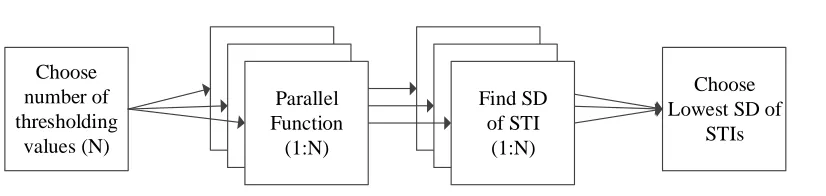
Figure 2.1 contains the generic model for the least variance adaptation of the processing

(26)

Choose number of thresholding

values (N)

Parallel Function (1:N)

Choose Lowest SD of

STIs Find SD

[image:26.612.112.525.102.200.2]

of STI (1:N)

Figure 2.1: The least variance adaptations of the historic algorithms follow similar flows: choose the number of iterations, run the algorithm with different tuning parameters, find the standard deviation of the STI, then choose the systolic time interval with the least variance.

2.1

ECG R-Wave Pulse Transit Time (rPTT)

The R-wave pulse transit time is the time duration between the ECG R-wave peak and the

PPG foot, where the R-wave peak is extracted by a simple peak detection algorithm and the

PPG foot is historically found by using the percent height algorithm found in commercial

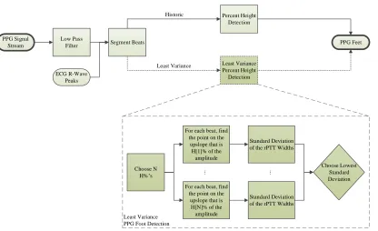
systems such as the SphygmoCor health monitoring system [20] (Figure 2.2).

2.1.1 Percent Height PPG Foot Detection

The algorithm for the percent height PPG foot detection starts by low pass filtering the raw

PPG signal, then segmenting it by using the robustly extracted ECG R-wave as the start of

each beat. The time value that is located at 5 percent of the total amplitude for that beat

is extracted, and the final rPTT value is found by using Equation 2.1, whereP P Gf ootis the

time that the PPG foot occurs, and ECGr−wave is the time that the R-wave peak occurs.

Note that the5 percent value is chosen based on the default value of the SphygmoCor health

monitoring system [20].

rP T T =P P Gf oot−ECGr−wave (2.1)

(27)

Least Variance PPG Foot Detection PPG Signal

Stream

Low Pass

Filter Segment Beats PPG Feet

Least Variance Percent Height Detection Percent Height Detection ECG R-Wave Peaks Choose N H% s

For each beat, find the point on the

upslope that is H[1]% of the amplitude

Standard Deviation of the rPTT Widths

For each beat, find the point on the

upslope that is H[N]% of the amplitude

Standard Deviation of the rPTT Widths

[image:27.612.108.524.95.349.2]

Choose Lowest Standard Deviation ... ... Historic Least Variance

Figure 2.2: The PPG foot detection is shown, with the percent height algorithm on the upper path, and the least variance adaptation on the lower, darker path.

thresholding level, since the noise will be extracted rather than the true PPG foot.

2.1.2 Least Variance PPG Foot Detection

Rather than thresholding at a fixed percentage, the threshold parameter was varied in the

least variance algorithms (Figure 2.1). The least variance PPG foot detection algorithm

thresholds across N percent heights, with the thresholded value containing the smallest

variance of rPTT values extracted as the PPG foot (Figure 2.2. The rPTT is then found

by Equation 2.1.

2.2

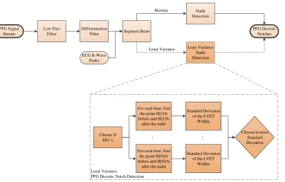
Left Ventricular Ejection Time (LVET)

The left ventricular ejection time is the time duration from the PPG foot to the PPG

dicrotic notch, where the PPG foot is found by using the percent height algorithm explained

(28)

by Quarry-Pigott [16] (Figure 2.3).

Least Variance

PPG Dicrotic Notch Detection PPG Signal

Stream

Low Pass

Filter Segment Beats

PPG Dicrotic Notches Least Variance Nadir Detection Nadir Detection ECG R-Wave Peaks Differentiation Filter Choose N H% s

For each beat, find the point H[1]% before and H[1]%

after the nadir

Standard Deviation of the LVET

Widths

For each beat, find the point H[N]% before and H[N]%

after the nadir

Standard Deviation of the LVET

[image:28.612.112.524.122.385.2]

Widths Choose Lowest Standard Deviation ... ... Historic Least Variance

Figure 2.3: The PPG dicrotic notch detection is shown, with the Quarry-Pigott algorithm on the upper path, and the least variance adaptation on the lower, darker path.

2.2.1 Quarry-Pigott PPG Dicrotic Notch Detection

The duration between the PPG foot and the PPG derivative nadir (dicrotic notch) after

the peak was identified as providing an accurate estimate of LVET [16]. To find the

di-crotic notch, the PPG signal is low-pass filtered, differentiated, low-pass filtered again, and

segmented into beats based on the ECG R-peaks. The nadir after the peak is taken as the

dicrotic notch, and the final LVET is found by using Equation 2.2, where dP P Gnadir is the

nadir of the PPG derivative signal, and the P P Gf oot is the foot of the PPG signal.

LV ET =dP P Gnadir−P P Gf oot (2.2)

The algorithm accuracy suffers when noise induces multiple zero-slope locations in the

(29)

2.2.2 Least Variance PPG Dicrotic Notch Detection

The nadir detection of the Quarry-Pigott algorithm was replaced with a thresholding

algo-rithm that varies on the upslope and downslope surrounding the nadir (Figure 2.1). The

least variance algorithm extracts N/2 percent heights on the downslope to the nadir, and

N/2 additional percent heights on the upslope after the nadir and the thresholded value

with the least variance of LVET values is extracted as the PPG dicrotic notch. The LVET

(30)

Chapter 3

CUDA

3.1

Graphics Card Background

A GPU, or graphics processing unit, is essentially a coprocessor that is able to perform

operations on pixel values, and can be either discrete or integrated. An integrated GPU

typically uses a portion of the memory on the host, and is usually slower than its discrete

counterparts. A discrete GPU is one that is mounted on a graphics card, which is a printed

circuit board containing the GPU, some amount of discrete memory, and an interface to

the computer’s motherboard.

Graphics cards were first produced for the public market in 1982, with Intel’s iSBX

275 Video Graphics Control Multimodule board [21]. This graphics card was able to draw

simple lines, rectangles, arcs, and text. It contained an onboard memory module, called

a frame buffer. This frame buffer was able to read and write to the host system memory

via DMA, or direct memory access. The processor would write the graphics card through

a custom API, or application programming interface. The graphics card would take those

commands, perform the corresponding logic to the pixels in the frame buffer, and output

the necessary signals to the monitor.

In the 1990s, graphics card producers, such as NVIDIA, ATI, and 3dfx, started releasing

abstractions to allow application developers to take advantage of the GPU through standard

programming languages. A few of these standard APIs include OpenGL, Glide API, and

DirectX. These APIs allowed programmers to code for any compatible graphics card, rather

(31)

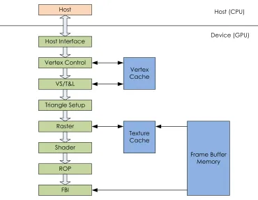
A typical graphics card produced in the mid to late 1990s contained a massively parallel

pixel pipeline. A single pixel pipeline had several stages in which the pixels were processed

through to render an image. These pixel pipelines were instantiated many times in the

GPU, in order to process many pixels together at the same time, in parallel. Figure 3.1

shows a fixed-function graphics pipeline from an early NVIDIA GeForce GPU. Commands

are sent from an application running on the host through a standard API. The host interface

received the commands and data from the CPU. It also contained hardware to perform direct

memory access (DMA) to transfer data in bulk from the main host memory to the graphics

pipeline. The other stages of the pipeline were essentially to perform transformations on

the final rendered image.

The NVIDIA GeForce 3, released in 2001, was the first graphics card to allow the

pixel pipeline to be programmable, meaning that the functionality of some of the stages

could be changed to produce different rendered pixels [22]. In particular, the floating-point

vertex engine (VS/T&L stage) was given programmability by publicly releasing the private

instruction set. This allowed for more control over how the final outputted image was

manipulated, but also gave a means of using this new architecture to perform calculations

on non-pixel data. This lead to a new way of GPU computing, now known as

(32)

Host

Host Interface

Vertex Control

VS/T&L

Triangle Setup

Raster

Shader

ROP

FBI

Vertex Cache

Texture Cache

Frame Buffer Memory

Host (CPU)

[image:32.612.115.485.99.386.2]

Device (GPU)

Figure 3.1: A Fixed-Function NVIDIA GeForce Graphics Pipeline

Computing data using the GPGPU architecture had its problems. For one, there were

no user-defined data types, meaning the programmer needed to store data within the vector

arrays on the GPU. Secondly, the primitive operations, such as addition, division, etc., were

not IEEE compliant. This meant that computations on a GPU were not necessarily the

same as that on a CPU, or even another GPU. Finally, the GPGPU pipeline did not provide

an easy way to write to the main memory; the computation needed to be converted to a

pixel color and saved to the frame buffer memory before it could be written to main memory.

These deficiencies of the GPGPU programming model led the way towards more powerful

(33)

3.2

NVIDIA’s CUDA

In 2007, NVIDIA released a set of graphics cards with an entirely new architecture. This

programming model and hardware was dubbed CUDA. Originally, CUDA stood for

com-pute unified device architecture. Like the GPGPU, it allowed for advanced programmability

of the graphics pipeline. However, instead of providing the APIs to program certain stages,

CUDA replaced the pipeline with fully programmable processors with instruction memory,

instruction cache, and instruction sequencing control logic. NVIDIA also added an abstract

parallel programming model with a hierarchy of parallel threads, as well as barrier

synchro-nization and atomic operations. To go along with this new architecture, the CUDA C/C++

compiler, library, and runtime software were developed to enable programmers to easily use

the new CUDA GPU architecture [23].

In 2010, NVIDIA released its newest version of the CUDA architecture called Fermi.

Fermi introduced several new features to increase parallel performance. This included new

streaming multiprocessors, an improved memory subsystem, and new application switching

logic. This work will use the Fermi-based CUDA architecture [24].

3.2.1 CUDA Threads

A typical CUDA program has two main parts: the sequential part that runs on the host

(CPU), and the parallel part that runs on the device (GPU). These two components work

together to perform some task. Usually, the sequential part will setup the GPU, load and

access the GPU’s memory, and start the parallel code. The parallel part, also known as a

kernel, will execute some small task that will run in parallel on many small processors within

the GPU. Each small task, which is also called a thread, is exactly the same. However, the

threads execute on different data. This programming model is known as “same program,

multiple data,” or SPMD, because the same program is processing multiple data values. For

CUDA, the SPMD programming model is identical to SIMD, or “same instruction, multiple

data,” since the same instruction is run in multiple threads on multiple data values.

CUDA also introduced abstract concepts known as blocks and grids. When a kernel is

launched, it creates a grid of thousands to millions of threads. In Figure 3.2, Kernel 0 on

(34)

When running a large number of threads in a grid, it is necessary to create a large amount

of data parallelism (more on parallelism is in a later section).

The grids are split up into a two-dimensional array of blocks. These blocks are further

organized into three-dimensional arrays of threads. Figure 3.2 shows an example of this

thread hierarchy. In this figure, each grid is split up into a 2 by 3 matrix of blocks. Each

block is then arranged into 2 by 4 by 2 matrices of threads. The number of threads shown

is very small compared to what would normally run on a GPU, but were kept small for ease

of describing the CUDA thread organization [23].

Host Device Grid 0 Block (0,0) Block (0,1) Block (1,0) Block (1,1) Block (2,0) Block (2,1) Grid 1 Block (0,0) Block (0,1) Block (1,0) Block (1,1) Block (2,0) Block (2,1) Kernel 0 Thread

(0,1,0) Thread(1,1,0) Thread(2,1,0) Thread(3,1,0) Thread

(0,0,0) Thread(1,0,0) Thread(2,0,0) Thread(3,0,0) (0,0,1) (1,0,1) (2,0,1) (3,0,1)

[image:34.612.107.515.268.648.2]

Kernel 1 Ex e c u tio n Tim e

(35)

Arranging threads into grids, blocks, and grids is the responsibility of the programmer.

It is their job to assign the threads correctly to assure the hardware resources of the

graph-ics card are fully utilized. In addition, there is a concept called warps that is an implied

responsibility of the programmer. Warps are not assigned by the programmer, but are

automatically created. Implied responsibility means that the programmer should

under-stand how these warps are created in order to choose the thread hierarchy to best use the

hardware on the CUDA card. Each block is assigned to a streaming multiprocessor (SM).

Multiple blocks may be assigned to a single SM if there are enough resources available.

These threads running on the SM are broken up into groups of 32 threads, called warps.

Within SMs, warps are the unit of thread scheduling.

As mentioned earlier, each warp contains up to 32 threads from the same block that

contain the same program counter. Because all 32 threads in a warp share the same program

counter, they all execute the same instructions simultaneously. However, even though each

thread shares a program counter, it is still possible for divergence within a warp. For

example, if a warp contains a branching instruction, such as an if-else construct, certain

threads may execute some instructions while others do not. In this case, the warp will

maintain an active mask to keep track of which threads in the warp will execute the next

instruction. This active mask can be used to disable threads that are not part of the current

branch path. Hence, the threads do notdiverge, but instead do not execute until the control

path converges again.

Figure 3.3 shows an example of how a streaming multiprocessor warp scheduler might

schedule warps. Note that only 16 instructions are shown for simplicity. In this example, all

threads in Warp 8 will execute instruction 22. Then, only 7 threads in Warp 1 will execute

instruction 63. This shows the warp divergence explained earlier. Warp 5 will then have all

threads execute instruction 12. The warps are scheduled based on which are ready to run,

and which are currently waiting. If, for example, one warp needed to access high-latency

global memory, it would be taken out of the priority schedule until it received its data from

(36)

Streaming Multiprocessor

Warp Scheduler

Warp (8); Instruction (22)

Warp (5); Instruction (13) ...

Ti

m

[image:36.612.124.500.108.597.2]

e

(37)

3.2.2 CUDA Architecture

Figure 3.4 shows the block diagram of a typical Fermi based CUDA-capable GPU. In essence,

the CUDA architecture contains hundreds of streaming processors, known as CUDA cores.

The CUDA cores are then grouped into streaming multiprocessors (SMs). The SMs are

positioned around a common L2 cache, with each SM having access to read and write to

both L2 cache and global DRAM memory.

In regards to the Fermi architecture, there are up to 512 streaming multiprocessors,

organized into groups of 16 SMs with 32 streaming processors each. The GigaThread warp

scheduler is in charge of assigning work to each of the SMs. Furthermore, there can be up

to 6 GB of GDDR5 DRAM memory, arranged into six partitions [24].

Device (GPU) Host Input Assembler GigaThread Load/ Store L2 Cache SPs, SFUs, LD/ST Regs/ Cache Dispatch SPs, SFUs, LD/ST Regs/ Cache Dispatch SPs, SFUs, LD/ST Regs/ Cache Dispatch SPs, SFUs, LD/ST Regs/ Cache Dispatch SPs, SFUs, LD/ST Regs/ Cache Dispatch SPs, SFUs, LD/ST Regs/ Cache Dispatch SPs, SFUs, LD/ST Regs/ Cache Dispatch Load/

Store Load/Store Load/Store Load/Store Load/Store Load/Store

DRAM

[image:37.612.106.516.314.600.2]

...

(38)

Streaming Multiprocessor

The streaming multiprocessors (SMs) are the main processing center for CUDA-capable

GPUs. Each SM is made up of several streaming processors (SP), warp schedulers,

dis-patch units, a register file, load and store units (LD/ST), special function units (SFU), an

interconnection network, shared memory, level one instruction cache, level one data cache,

and level two uniform data cache. Figure 3.5 shows the typical block diagram for the

streaming multiprocessor.

In the Fermi architecture, there are up to 512 streaming multiprocessors. Within each

SM will be 32 streaming processors, 16 load and store units, four special function units, two

warp schedulers, two dispatch units, a 32K x 32-bit register file, and a 64K memory that is

(39)

L1 Instruction Cache

Warp Scheduler Warp Scheduler

Dispatch Unit Dispatch Unit

Register File (32 KB x 32-bit)

Interconnection Network

Shared Memory and L1 Cache (64 KB)

L2 (Uniform) Cache

[image:39.612.110.517.100.489.2]

LD/ST SFU SFU SP SP SP SP Dispatch Port Operand Collector Result Queue FPU ALU SP SP SP SP SP SP SP SP SP SP SP SP SP SP SP SP SP SP SP SP SP SP SP SP SP SP SP SP SP LD/ST LD/ST LD/ST LD/ST LD/ST LD/ST LD/ST LD/ST LD/ST LD/ST LD/ST LD/ST LD/ST LD/ST LD/ST SFU SFU

Figure 3.5: Architecture of a Fermi Streaming Multiprocessor, adapted from [24]

Streaming Processor Each streaming processor (SP), or CUDA core as they are

typ-ically called, is essentially a low-speed processor. However, where a CPU runs between

one and sixteen threads simultaneously, a GPU can run upwards of thousands of threads

in parallel. Thus, a GPU is said to have “strength in numbers,” meaning the GPU can

break up a task into many small computations in order to obtain better performance than

a high-powered CPU.

(40)

instructions, the operand collector for receiving the operands, the floating point unit (FPU)

that uses the IEEE 754-2008 floating point standard, the fully pipelined 32-bit integer

arithmetic logic unit (ALU), and the result queue for sharing its results with the other

parts of the SP [24].

Register File A register file is contained within each streaming multiprocessor. Each

thread contains its own set of local registers within the register file. The amount of registers

each thread owns depends on how many registers each thread requires. In this sense, the

registers are dynamically allocated. Once the registers have been allocated to a specific

thread within a SM, those registers cannot be accessed by another thread.

By allowing the registers to be dynamically allocated, it allows more flexibility to both

the compilers and the programmers. The compilers have more freedom to tradeoff between

instruction-level parallelism and thread-level parallelism. Instruction-level parallelism is the

parallelism that exists between instructions within a thread. Thread-level parallelism is the

parallelism between multiple threads. The compiler can choose whether the best speedup

will occur when instruction-level parallelism or thread-level parallelism is exploited. The

programmer can choose how many registers each thread should have, allowing more or less

threads running on each SM. By giving the programmer control over the number of threads

on each SM, it gives the opportunity for better execution times [23].

The Fermi-based register file is 32 KB long by 32-bits wide. By making the width 32

bits, it allows for floating-point numbers to be easily stored in a single register [24].

Warp Scheduler The dual warp schedulers within the streaming multiprocessors are

used to schedule which warps should execute next. Warps are added to the scheduler when

all of its operands are ready for consumption for the next execution cycle. Eligible warps

are selected based on a prioritized scheduling policy. In other words, the warp scheduler has

logic to decide which warp is of higher priority. This logic is a combination of round-robin

scheduling, and age of warp scheduling [23].

Round-robin scheduling is a scheduling algorithm where time slices are assigned to each

task in a cyclic pattern. In this algorithm, the tasks do not have priority, meaning each

(41)

another scheduling algorithm where tasks are assigned based on the age of the task. With

this algorithm, older tasks will have a greater chance of running next than younger tasks.

By combining these two scheduling algorithms, the Fermi CUDA architecture will perform

round-robin scheduling for each age group. For example, the oldest tasks will execute in

round-robin, then the next oldest tasks will run in round-robin, and so on.

As stated earlier, each thread in a warp executes the same instruction. To keep track

of which threads should be active during a specific instruction, the warp scheduler contains

active masks for each warp in the streaming multiprocessor. When a thread should not be

active on a certain program counter, the bit in the active mask for that thread is cleared,

telling the dispatch unit to skip dispatching that thread for the current instruction [23]

Unlike other scheduling systems, the warp scheduler does not introduce any latency

when switching warps. This concept is called zero-overhead thread scheduling. The only

time that warp switching causes an overhead is when there are no warps available to run

because the operands to every warp are not available. To remedy this, simply introduce

more threads in each block to create more warps. This way, there are more warps, allowing

other warps to execute while others are waiting for long-latency memory operations to

complete [24].

In the Fermi-based CUDA cards, there are two warp schedulers. Each scheduler chooses

a separate warp to be issued and executed concurrently. The schedulers then issues one

instruction from each warp to either the groups of SPs, the load and store units, or the

SFUs. Because the two warp schedulers operate on separate warps, there is no need to check

for dependencies between them. This allows for excellent, near-peak hardware performance

when executing [24].

Dispatch Unit The dispatch unit is used to fetch instructions from L1 instruction cache,

and dispatch those instructions to the correct streaming processors according to the warp

schedulers. The dispatch unit is tightly coupled with the warp scheduler, in that it is the

interface between scheduling the warps and the streaming processors. As previously

men-tioned, there are two warp schedulers and two dispatch units in Fermi-based architectures

(42)

Load and Store Control The load and store control units within the streaming

multi-processors are used as the interface between the threads and the memories. These memories

include the register file, the shared memory and L1 cache, the local L2 cache, the global L2

cache, and the global DRAM memory [24].

Special Function Units The special function units (SFUs) are specialized arithmetic

units that are able to perform mathematical functions such as sine, cosine, reciprocal, and

square root. The SFUs are decoupled from the execution pipeline, meaning other warps

may be dispatched to the streaming processors while the SFUs are occupied. In Fermi-based

CUDA cards, there are four SFUs per SM, double that of previous CUDA architectures [24].

Shared Memory and L1 Data Cache Shared memory is a chunk of memory that can

be accessed by every thread executing on a single streaming multiprocessor. This is useful

for programs that require knowledge of the data around the data point it is currently working

on, such as matrix calculations. Shared memory is ideal to use in these situations because

accessing shared memory takes a very short amount of time compared to accessing global

DRAM. Once shared memory is loaded, it is significantly faster than accessing DRAM, and

can be accessed by multiple threads [24].

Level one (L1) cache is a new feature on Fermi-based CUDA cards. It is used to hold

global memory references, to decrease DRAM access times. This type of cache is very

useful when the kernel may not be accessing data locations that can be shared between

other threads [25].

In Fermi architectures, there is 64 KB of configurable memory in each streaming

mul-tiprocessor. This memory can be configured as 48 KB of shared memory and 16 KB of

L1 cache, or 16 KB of shared memory and 48 KB of L1 cache. The choice is that of the

programmer and depends on two factors: how much shared memory is needed, and how

predictable are the kernel’s accesses to global memory likely to be [25].

L2 Data Cache (Local) The Fermi architecture added L2 cache to each streaming

multiprocessor. This cache allows for faster accesses to DRAM. An important feature of

(43)

are uninterruptible. These atomic operations are ideal for accessing shared data locations;

this includes data shared between blocks, or kernels. By implementing atomic operations

in hardware, it allows the ALU to perform the operation without having to us semaphores

[25].

GigaThread Scheduler

The GigaThread scheduler is in charge of distributing thread blocks to the SMs. The input

assembler on the host will compile the input code into an instruction set that the scheduler

can understand. Said scheduler will take the instructions and split up the work based

on the kernels already running on the GPU. Thus, multiple kernels can run on the same

CUDA card, with near-instantaneous kernel switching (under 25 microseconds), due to the

capabilities of the GigaThread scheduler [24].

L2 Cache and DRAM

The level 2 cache (L2) and dynamic random access memory (DRAM) memories are known

as the global memories on the Fermi GPU. These memories, unlike the local memories, can

be accessed by every SP within the GPU. Thus, the global memories make it useful for

inter-thread communication on a per-application basis. However, as explained earlier, accessing

global memory is typically slower than accessing local memory. Using global memory is a

tradeoff between communicating between processors and speed.

As seen from its name, L2 cache is used to cache accesses to DRAM. When memory is

accessed in DRAM, those values are transfered to L2 cache for future reference. This is

im-portant for memory coalescing. Memory coalescing is when memory is accessed sequentially.

For example, a warp may access memory locationsM0,0, M1,0, M2,0, M3,0 in that order. This

will have a far greater access time than if the warp accessed M0,0, M10,3, M4,2, M0,20. This

is because DRAM cells are essentially weak capacitors. When these cells are accessed, the

small charge on the capacitor must be shared with a sensor to set off a comparator circuit

to determine if that cell had a zero or a one present on it. Since this is a slow process due to

the small charges on the capacitors, most modern DRAMs use a parallel process to increase

(44)

same time, and compare each of the charges in parallel. The DRAM then transfers the

data from each location at high speed to the cache [23]. Thus, reading consecutive global

memory locations will give a much higher bandwidth than reading random data locations.

3.3

Data Parallelism

Data processing on graphics cards is used primarily when there are a large number of

computations that have low data dependencies. For example, Listing 3.1 would be a good

candidate for implementing on a graphics card. In this C-like example, two arrays,bandc,

are added together and placed in array a. These arrays are added by looping through each

value of b and c and adding the values at that location together, putting the sum in the

corresponding location in a. This is a good candidate for parallelizing with a GPU since

there is no data dependencies between iterations of the for loop.

Listing 3.1: Typical GPU Algorithm: Vector Addition

1 // - N is the s i z e of a r r a y s b and c

2 // - A r r a y a is a l r e a d y pre - a l l o c a t e d

3 // - A r r a y s b and c c o n t a i n n u m b e r s

4 for (int i = 0; i < N ; i ++) {

5 a [ i ] = b [ i ] + c [ i ];

6 }

In order to write code that will execute quickly and correctly in parallel on a GPU, it is

important to understand the data dependencies between computations. The sections that

follow will explain the three types of data dependencies in more detail.

3.3.1 Flow Dependency

Flow dependency occurs when a task depends on the result of a previous task. Listing 3.2

shows an example of something that has a flow dependency. When the loop is on a given

iteration (i), array arequires the value of a from the previous iteration (i−1). Thus, the

(45)

Listing 3.2: Flow Dependency Example

1 for (int i = 1; i < N ; i ++) {

2 a [ i ] = a [ i -1] + b [ i ];

3 }

3.3.2 Anti-dependency

Anti-dependency occurs when a task depends on a value that is later changed. Listing 3.3

shows an example of something that has an anti-dependency. In this example, arrayauses

the value ataof the next loop iteration. On the next value ofi,a[i+1]will be overwritten,

meaning the a[i]is anti-dependent on a[i+1].

Listing 3.3: Anti-dependency Example

1 for (int i = 0; i < N ; i ++) {

2 a [ i ] = a [ i + 1 ] ; + b [ i ]

3 }

3.3.3 Output Dependency

Output dependency occurs when the ordering of the tasks affect the result. Listing 3.4

shows an example of something that has an output dependency. Array a is the sum of

arrays b and c. However, array c is also assigned the sum of arrays d and e. If lines 2

and 3 were swapped, the value of array a would change, meaning that there is an output

(46)

Listing 3.4: Output Dependency Example

1 for (int i = 0; i < N ; i ++) {

2 a [ i ] = b [ i ] + c [ i ];

3 c [ i ] = d [ i ] + e [ i ];

4 }

3.4

CUDA Programming Structure

CUDA is the hardware and software architecture that allows NVIDIA GPUs to execute

programs written in high-level languages, such as C, C++, Fortran, and more. A typical

CUDA program will have code that executes on the CPU, or the host, as well as on the

GPU, or the device. The code that runs on the device is known as a kernel. A kernel will

execute in parallel across many threads simultaneously. These threads may be organized in

grids of blocks of threads by the programmer or the compiler.

Usually, a CUDA program will consist of phases, where the code with little data

paral-lelism is executed on the host, and those with a lot of data paralparal-lelism is executed on the

device. Figure 3.6 shows this phenomenon. In this figure, the CUDA program starts out

executing the code serially on the CPU. Then, a kernel is called to run in parallel on many

threads. The CPU then runs some code in serial, until another kernel is called to run more

(47)

Grid (0)

…

Thread Thread Thread Thread

Grid (1)

…

Thread Thread Thread Thread

CPU Serial Code

GPU Parallel Kernel

CPU Serial Code

GPU Parallel Kernel

Serial Code

[image:47.612.117.514.96.398.2]

Serial Code

Figure 3.6: Execution of a Typical CUDA Program, adapted from [23]

Listing 3.5 shows an example CUDA program that will add two arrays element-wise.

This code follows the programming pattern shown in Figure 3.6; the CPU code (int ...

main()) will first run in serial. The serial code will setup the device kernels, and start executing those kernels (add dev(...)). This example was adapted from Sanders and

(48)

Listing 3.5: Example CUDA Code

1 # d e f i n e N = 64

2 /* C o d e t h a t r u n s on the d e v i c e ( GPU ) */

3 _ _ g l o b a l _ _ v o id a d d _ d e v (int * a , int * b , int * c ) {

4 int t h r e a d I d = b l o c k I d x . x ; // The i n d e x of the t h r e a d e x e c u t i n g 5 // Add the e l e m e n t s c o r r e s p o n d i n g to the i n d e x of the c u r r e n t t h r e a d

6 if ( t h r e a d I d < N ) {

7 c [ t h r e a d I d ] = a [ t h r e a d I d ] + b [ t h r e a d I d ];

8 }

9 }

10 /* C o d e t h a t r u n s on the h o s t ( CPU ) */

11 int m a i n () {

12 int a [ N ] , b [ N ] , c [ N ]; // H o s t ( CPU ) a r r a y s 13 int * a_dev , * b_dev , * c _ d e v ; // D e v i c e ( GPU ) p o i n t e r s 14 // A l l o c a t e m e m o r y on the d e v i c e

15 c u d a M a l l o c( (v o i d**) a_dev , N * s i z e o f(int) ) ;

16 c u d a M a l l o c( (v o i d**) b_dev , N * s i z e o f(int) ) ;

17 c u d a M a l l o c( (v o i d**) c_dev , N * s i z e o f(int) ) ;

18 // F i l l h o s t a r r a y s a and b w i t h d a t a h e r e

19 /*

20 */

21 // C o p y a and b to the d e v i c e

22 c u d a M e m c p y( a_dev , a , N * s i z e o f(int) , c u d a M e m c p y H o s t T o D e v i c e ) ;

23 c u d a M e m c p y( b_dev , b , N * s i z e o f(int) , c u d a M e m c p y H o s t T o D e v i c e ) ;

24 // E x e c u t e a d d _ d e v on the d e v i c e

25 add_dev < < N ,1 > >( a_dev , b_dev , c _ d e v ) ;

26 // C o p y c _ d e v f r o m the d e v i c e b a c k to the h o s t

27 c u d a M e m c p y( c , c_dev , N * s i z e o f(int) , c u d a M e m c p y D e v i c e T o H o s t ) ;

28 // F r e e the m e m o r y on the d e v i c e

29 c u d a F r e e( a _ d e v ) ;

30 c u d a F r e e( b _ d e v ) ;

31 c u d a F r e e( c _ d e v ) ;

(49)

3.5

MATLAB to CUDA Compilation

With the advent of MATLAB’s Parallel Computing Toolbox, it is now possible to write

MATLAB programs to take advantage of NVIDIA’s CUDA graphics cards. There are

several ways to write MATLAB code to speed up computations on a GPU. One of which is

to use overloaded built-in function calls. Another is to write a kernel in MATLAB to run

on each element of a large matrix. A final way is to write CUDA code that can be called

from MATLAB [27].

For each of the methods of writing parallel code to be used with MATLAB, it is

im-portant to keep a few things in mind. First, it is imim-portant to understand the hardware

inside the graphics card. Without a good knowledge of how many streaming processors, how

much memory, and the limitations of GPU, it is very difficult to receive optimal performance

from the code. Second, it is important to understand the data dependencies between

com-putations, When these dependencies are violated, stalls will appear in the CUDA pipeline,

causing enormous slow-downs in the program. Finally, it is important to understand the

pros and cons of the three ways of writing CUDA code for MATLAB. The three sections

below will explain the methods, as well as detail when each should be used.

3.5.1 MATLAB Function Overloading

MATLAB has support for overloading function calls with GPU function calls. Instead of

calling a function on a CPU array, it would be called on a GPU array. For example, in

Listing 3.6, a fast Fourier transform (FFT) is performed on two random arrays. TheAarray

is located on the CPU, and the GAarray is located on the GPU. The same function call is

used for both arrays: fft(). However, sinceGA is located on the graphics card, thefft()

function is executed as a CUDA kernel on the GPU and sinceAis located on the CPU, the

(50)

Listing 3.6: MATLAB Overloaded Functions

1 % S e r i a l

2 A = r a n d( 2 ^ 1 2 , 1 ) ;

3 B = fft( A ) ;

4 % P a r a l l e l

5 GA = g p u A r r a y(r a n d( 2 ^ 1 2 , 1 ) ) ;

6 GB = fft( GA ) ;

7 GC = g a t h e r( GB ) ;

With all MATLAB code that runs on a GPU, it is important to note that GPU arrays

must be copied back to the CPU before they can be used by a CPU function. In Listing 3.6,

the gather()function is used to copy theGBarray back to the CPU.

MATLAB function overloading is the easiest to implement in existing MATLAB code

because it requires the fewest code changes. As long as the existing serial code uses

sup-ported overloaded functions, the changes to convert it to parallel code is minimal; simply

use gpuArray() to send the arrays to the GPU, and gather() to bring the arrays back

to the CPU. In Tordoff’s Mandelbrot experiment, using overloaded functions resulted in a

speedup of around 16 times that of the CPU code [28].

3.5.2 MATLAB Kernels

In MATLAB, it is possible to write a function that will perform a task on a single element

of an array. By running this MATLAB function on the GPU, it becomes very similar to

running a CUDA kernel, except is is written in MATLAB.

Listing 3.7 shows an example of using the arrayfun function to execute gpuPlus()

on each element of Ga and Gb. In this example, gpuPlus()will add elements of the same

index from both of the input arrays. Since Ga and Gb are both GPU arrays, gpuPlus()

(51)

Listing 3.7: MATLAB Kernels

1 % F u n c t i o n

2 f u n c t i o n [ o ] = g p u P l u s ( a , b ) ;

3 o = a + b ;

4 end

5

6 % C o d e

7 Ga = g p u A r r a y(r a n d( 2 0 0 ) ) ;

8 Gb = g p u A r r a y(r a n d( 2 0 0 ) ) ;

9 Go = a r r a y f u n( @ g p u P l u s , a , b ) ;

10 o = g a t h e r( Go ) ;

MATLAB kernels are more in depth to implement than using overloaded functions. It

is necessary to create the element-wise function, and call it usingarrayfun(). In Tordoff’s

Mandelbrot experiment, using element-wise MATLAB kernels provided a speedup of 164

times that of the serial CPU code [28].

3.5.3 MATLAB CUDA Kernels

The final way to execute MATLAB code on a CUDA-capable graphics card is to write a

custom CUDA kernel, then execute the pre-compiled code with existing MATLAB bindings.

Listing 3.8 shows the CUDA code. This code is then compiled into the ptx file, which is

essentially the binary that runs on the CUDA card. Listing 3.9 is the MATLAB code that

will initialize the GPU arrays, create the kernel in MATLAB, run the kernel, and save the

(52)

Listing 3.8: CUDA Kernel Example

1 // C U D A C o d e ( m u s t be c o m p i l e d )

2 _ _ g l o b a l _ _ v o i d a d d _ d e v (c o n s t d o u b l e * a , c o n s t d o u b l e * b , d o u b l e ...

* c ) {

3 int t h r e a d I d = b l o c k I d x . x ; // The i n d e x of the t h r e a d e x e c u t i n g 4 // Add the e l e m e n t s c o r r e s p o n d i n g to the i n d e x of the c u r r e n t t h r e a d

5 if ( t h r e a d I d < N ) {

6 c [ t h r e a d I d ] = a [ t h r e a d I d ] + b [ t h r e a d I d ];

7 }

8 }

Listing 3.9: MATLAB CUDA Kernels

1 % % M a t l a b c o d e

2 % I n i t i a l i z e the GPU a r r a y s

3 Ga = g p u A r r a y(r a n d(200 ,1) ) ;

4 Gb = g p u A r r a y(r a n d(200 ,1) ) ;

5 % C r e a t e the k e r n e l in M A T L A B

6 k = p a r a l l e l . gpu . C U D A K e r n e l ('a d d _ d e v . ptx','a d d _ d e v . cu' ) ;

7 k . T h r e a d B l o c k S i z e = 2 0 0 ;

8 % Run the k e r n e l and c o p y the r e s u l t to the CPU

9 Go = f e v a l( k , Ga , Gb ) ;

10 o = g a t h e r( Go ) ;

MATLAB CUDA kernels require the most effort to run with MATLAB. It is necessary

to understand the subset of CUDA that is available to use with MATLAB. It is also required

to format the input parameters in such a way that MATLAB is able to create the kernel

and its inputs and outputs correctly. CUDA code must also be compiled first before it

can be used, unlike typical MATLAB code. Although this is more difficult to execute, it

does provide the most flexibility and has the largest potential for speedup. In Tordoff’s

Mandelbrot experiment, using CUDA kernels gave a speedup of approximately 340 times

(53)

3.6

Potential Speedup

A simple script was written in MATLAB to examine the potential speedup of using

over-loaded functions. The hypothesis was that running with the GPU will provide a speedup

over running with a CPU for larger datasets. For smaller datasets, the time to load the

GPU arrays would be too large for the speedup of the actual function to overcome.

The function chosen was thefft() function. This was chosen because it was expected

that the fft would need to be run multiple times in the least variance algorithms. The

code is shown below in section 3.10.

Listing 3.10: gpu test.m

1 clear all;

2

3 N = 23;

4 N2 = 15;

5

6 disp('CPU')

7 t = zeros(1,N);

8

9 for n = 1:N %#ok<FORPF>

10 tic

11 A = rand(2ˆn, 1);

12 B = fft(A); %#ok<SNASGU>

13 t(n) = toc;

14 end

15

16 disp('GPU')

17 t gpu = zeros(1,N);

18

19 for n = 1:N %#ok<FORPF>

20 tic

21 A gpu = gpuArray(rand(2ˆn, 1));

22 B gpu = fft(A gpu); %#ok<SNASGU>

23 t gpu(n) = toc;

24 end

25

26 fig = figure('Name', 'Array Size Plot', 'NumberTitle', 'off');

27

28 set(fig, 'Color', 'w');

[image:53.612.95.538.309.712.2]

(54)

30 hold on;

31 plot(1:N,t, 'b', 'LineWidth', 1);

32 plot(1:N,t gpu, 'r', 'LineWidth', 1);

33 hold off;

34 title('FFT of Random Arrays')

35 xlabel('Array Size (2ˆN)')

36 ylabel('Time (s)');

37 box on;

38 legend('CPU', 'GPU', 'Location', 'SouthWest');

39

40 % Graph Insert

41 set(fig,'DefaultAxesFontSize', 8);

42 axes('Position', [.2,.65,.2,.2]);

43 hold on;

44 plot(1:N2,t(1:N2), 'b', 'LineWidth', 1);

45 plot(1:N2,t gpu(1:N2), 'r', 'LineWidth', 1);

46 hold off;

47 xlabel('Array Size (2ˆN)');

48 ylabel('Time (s)')

49 box on;

50

51 export fig(fig, 'gpu timing.pdf');

52

53 close(fig);

54

55 clear all;

The results from this test showed that the GPU executed thefftfaster than the CPU

for arrays larger than 215elements. For arrays smaller than that, the CPU performed faster.

This is expected, since the GPU must first copy the elements to the graphics card before

performing the fft. Figure 3.7 shows a plot of the execution time versus the size of the

array. The inset shows the time between arrays of 21 to 215 elements. This was added since

(55)

0

5

10

15

20

25

0

0.05

0.1

0.15

0.2

0.25

0.3

0.35

FFT of Random Arrays

Array Size (2

N

)

Time (s)

CPU

GPU

0 5 10 15

0 1 2 3

x 10−3

Array Size (2N)

[image:55.612.98.521.95.451.2]

Time (s)

(56)

Chapter 4

Methods

4.1

Data Collection

The physiological datasets used to verify the least variance algorithms were obtained

un-der informed consent using protocols approved by the Rochester Institute of Technology

Institutional Review Board for Protection of Human Subjects. The Biopac MP36 (Biopac

Systems, Inc., Goleta, CA) captured synchronized three-lead ECG and infrared ear PPG

from 15 subjects (60/40 male-to-female ratio) at a sampling rate of 50 kHz.

To vary the physiological states of the subjects, one minute measurements were captured

after pedalling four minutes at different activity levels, varied via the Life Fitness 95R1

Recumbent Bike. Measurements were taken at five levels of increasing resistance (L1, L2, L3,

L5, L7), then two levels of decreasing resistance (L3, L1), and a final recovery measurement

was taken after resting four minutes (REC). Repeat measurements were obtained on three

occasions, separated by 1-2 days.

4.2

Processing

Figure 4.1 contains the block diagram of the run_files.m script. All of the code can be

(57)

Run File Start Load Waveforms

Filter Waveforms

Segment/ Average Beats

Run File Complete Feature

[image:57.612.116.510.112.139.2]

Detection

Figure 4.1: The run files.m block diagram.

To process the physiological datasets, scripts were written using MATLAB (MathWorks,

Inc., Natick, MA). Datasets were downsampled to 500 Hz to approximate a clinical sampling

frequency [29] and reduce processing time. The PPG was low-pass filtered at 20 Hz with a

501-tap finite impulse response filter (FIR), then differentiated (9-tap differentiation filter),

and low-pass filtered at 20 Hz again (501-tap FIR). The ECG was bandpass filtered between

0.05 Hz and 150Hz (501-tap FIR), then notch filtered between 55 Hz and 65 Hz

(500-tap FIR) for line noise suppression. Filter types were selected based on prior algorithm

implementations [9, 16, 18, 30].

The signals were segmented into beats based on the R-wave peaks. PPG feet were

obtained from the 5-percent historic percent height method as well as the least variance

algorithm (N = 50, thresholds evenly spaced between 0 and 50 percent), and the PPG

dicrotic notches were captured with the historic Quarry-Pigott algorithm as well as the

least variance algorithm (N= 50, thresholds evenly spaced from 0 to 50 percent).

Figure 4.2 graphically shows how the beats were segmented with more detail. The chop

points for the peaks were shifted backwards in time 15 percent of the estimated beat length

from the ECG R-wave peaks. Each beat was then averaged with the next 10 beats in a

moving average algorithm, which assumes that the ECG and PPG signals are stable and

reproducible on a beat-to-beat basis. This was done to increase the signal-to-noise ratio of

(58)

1

2 3 4 5

s s s s s s

ecg

beat ecg

chop_pts r_peaks

1

2

3

4

5

ecg_seg(1,:)

ecg_seg(2,:)

ecg_seg(3,:)

ecg_seg(4,:)

ecg_seg(5,:)

[image:58.612.113.493.97.348.2]

segment_len

Figure 4.2: The waveforms of the 60 second dataset were segmented into beats, based on the ECG R-Peaks (red). The chop points (green) were found by shifting the R-peaks back 15 percent of the beat length. The end result is shown by the light blue arrows beneath the waveforms on the left, and is shown by the stack of beats on the right.

4.3