On modelling insights for emerging engineering problems : a case study on the impact of climate uncertainty on the operational performance of offshore wind farms

On Modelling Insights for Emerging Engineering

Problems: A case study on the impact of climate

uncertainty on the operational performance of offshore

wind farms

Iain Dinwoodie

, David McMillan

, Iraklis Lazakis

, Yalcin Dalgic

and

Matthew Revie

1 _{Institute for Energy and Environment, Department of Electronic and Electrical Engineering, University of}

Strathclyde, Glasgow, UK

2 _{Department Naval Architecture, Ocean and Marine Engineering, University of Strathclyde, Glasgow, UK} 3 _{SEATEC CO}

4 _{Department of Management Science, University of Strathclyde, Glasgow, UK}

Correspondence

D. McMillan, Institute for Energy and Environment, University of Strathclyde, Glasgow, UK

ABSTRACT

This paper considers the technical and practical challenges involved in modelling emerging

engineering problems. The inherent uncertainty and potential for change in operating environment

and procedures adds significant complexity to the model development process. This is

demonstrated by considering the development of a model to quantify the uncertainty associated

with the influence of the wind and wave climate on the energy output of offshore wind farms which

may result in sub-optimal operating decisions and site selection due to the competing influence of

wind speed on power production and wave conditions on availability. The financial profitability

of current and future projects may be threatened if climate uncertainty is not included in the

planning and operational decision making process. A comprehensive climate and wind farm

operational model was developed using a time series Monte Carlo simulation to model the

performance of offshore wind farms, identifying non-linear relationships between climate,

availability, energy output and capacity factor. This model was evaluated by engineers planning

upcoming offshore wind farms to determine its usefulness for supporting operational decision

making. From this, new consideration was given to the challenges in developing and applying

complex simulations for emerging engineering problems.

1. INTRODUCTION

In Europe alone, there is over 8GW installed capacity of offshore wind with ambitions to expand

this to over 40GW in the next decade [1]. To achieve this level of deployment, a number of

technological and economic challenges must be overcome. These include improving the

operational performance at turbine and wind farm level and successful integration of large amounts

of variable power output from wind farms into the wider electricity network. To overcome these

wind farms is needed. One area that has not been explored in detail is the extent to which wind

farm availability and power production is influenced by the wind and wave environment.

Operational performance of wind farms is typically measured by considering availability

(time-based) and capacity factor. Capacity factor in the context of an offshore wind farm is the ratio of

actual energy output relative to its potential output if it operated at its nameplate capacity over the

same period. Onshore, wind farm availabilities above 98% are achievable [2] and capacity factor

is therefore principally driven by wind resource. A more complex relationship exists in the offshore

environment between performance and climate conditions. This is due to high dependency on

vessel access for maintenance, which is primarily affected by wave height and wind speeds. As

increased wind speeds offshore are correlated to increased wave height, wind farms that are

positioned in sites with high wind resource, i.e. high wind speeds, will lead to lower accessibility.

This has resulted in lower availability but higher capacity factors than onshore, as observed at early

UK sites [3].

In order to reduce the uncertainty associated with the operational performance of future offshore

wind farms and to reduce the risks to the energy networks that they will be integrated into, a

rigorous analysis of the impact of climate uncertainty on availability and capacity factor is

required. This will not only impact planning decisions related to site selection but also influence

the infrastructure decisions required during a wind farms operation. Over time, a sufficiently varied

and detailed operational record linking wind speed, wave climate, availability and power

production may be acquired from existing wind farms. However, this may not emerge due to

commercial sensitivity and waiting for sufficient experience will result in significant delays to the

industry, additionally, there is currently no framework for publically disseminating performance

been developed for modelling aspects of offshore wind farms [4], none of these have considered

offshore climate uncertainty impact on capacity factor.

This research was motivated through discussions with Operations and Maintenance (O&M)

engineers, planners and economists on upcoming challenges in the offshore wind sector. One

reoccurring challenge was understanding the trade-offs that were being made during planning to

maximise power production against decreased availability. A flexible and intuitive modelling

approach was required that allowed decision makers to quickly model power production of an

upcoming wind farm configuration, encompassing the different range of information sources

available to them, while capturing all the uncertainty, both epistemic and aleatory, within the

problem. This paper illustrates this model through analysis on climate uncertainty using a base

case offshore wind farm [5]. The past development of O&M models for offshore wind is not

covered in this paper. Interested readers are referred to references [2, 4, 5].

Our research goal is a pragmatic one. We aim to develop an operational model that can support

decision making through improved understanding of the different decision levers available to

offshore wind farm operators during the planning stage while understanding how these decision

impact power production and resource requirements during the operational life of the wind farm.

Through this process we aim to reflect on the challenges with implementing such a solution within

organisations, particularly as the method adopted, Monte Carlo simulation, is widely applied

within risk analysis [6].

The modelling requirements and the developed model are described in Section 2. Section 3

presents a detailed investigation into the influence of wind and wave climate on the availability

and power production of a reference offshore wind farm. In Section 4 we reflect on the modelling

2. MODEL DESCRIPTION

There is a requirement for transparent Operating Expenditure (OPEX) models of varying degrees

of complexity that can be used for benchmarking and rigorous sensitivity analysis [7]; the model

outlined in this paper represents a detailed simulation model for this purpose. Previous academic

models in the field have principally adopted two approaches; simulation approaches, and direct

analytical methods. While direct methods are more computationally efficient, they often fail to

adequately describe the complexity of the system being modelled [8, 9]. Due to the non-linear,

highly complex and uncertain nature of the failure and repair process, lost revenue, maintenance

resource, operating climate etc., alternative approaches such as Monte Carlo simulation are often

applied [10-13]. These models, while computationally intensive, are able to capture a wider range

of uncertainties inherent in the problem [14, 15].

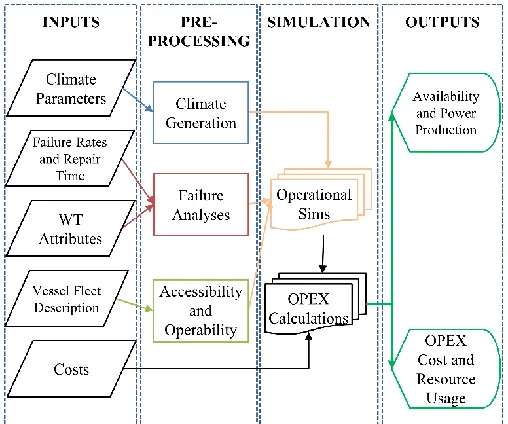
An outline of the resulting model is shown in Fig. 1 and described in the remainder of this section.

Climate parameter inputs comprise wind speed, wave height and wave period. All parameters are

used to determine accessibility and wind speed is used to determine wind farm power production.

Unlike onshore sites where high quality data sets of climate conditions are available, wind and

wave data at offshore sites is sparse. In addition, measurement campaigns, which are required for

project financing, are expensive for offshore projects and typically comprise a few years rather

than the expected operating lifetime of 20-25 years. Using the small sample period for all

simulations will fail to capture the variability and associated uncertainty of real world performance

over the life of a wind farm. It is therefore necessary to be able to produce representative synthetic

climate time series that can cover the duration of the wind farm life from smaller data sets. This

can be achieved by using a Multivariate Auto Regressive (MAR) climate model[14]. Key climate

characteristics for this application are annual mean, variance and distribution, persistence,

seasonality and critically, correlation between parameters.

The general form of an MAR model, normalized by the mean of the data μ is shown in (1), where

Xt is the simulated data at time step t, φ is the auto-regressive co-efficient, p is the model order

and E is a random noise covariance matrix. In order to apply (1) to a time series data set, the data

set mean and variance must be stationary and approximate a Gaussian distribution. Neither wind

speed nor wave period and height time series meet these criteria and therefore pre-processing is

required before a synthetic time series can be generated using (1). For the wind time series, removal

of seasonality and diurnal has been shown to be appropriate [16]. For the wave time series, it is

necessary to apply the Box-Cox transformation described in (2) or (3) where 𝜇̂ represents a

seasonal Fourier series fit of the transformed data and Λ is a transfer co-efficient in the range -1:1

Having transformed the data, (1) can be applied to both wind and wave data with the covariance

E replacing the independent random noise term and preserving the observed correlation in the

untransformed data. The determination of AR coefficients and model generation is implemented

using the arfit algorithm in MATLAB [18]. Order is chosen by optimizing Schwarz's Bayesian

Criterion and coefficients are estimated using a stepwise least squares estimation process. The

transfer co-efficient is optimized based on minimizing the skewness of the data set.

Failure rates and repair times inputs specify the reliability characteristics of the modeled system;

failure rate and repair time. Wind turbine (WT) attributes define the type and number of wind

turbines. A thorough discussion on reliability of offshore wind farms is presented in [19] covering

both wind farm and power system reliability. The failure analysis in this paper is related to the

wind farm level performance, but has wider applications on system level planning and reliability.

The methodology of the failure analyses block can be extended to cover wind farm level

components such as substations or to represent degradation of individual subsystems. Failure

behavior is implemented based on the methodology described by [20] and extended to wind farm

availability analysis in [21]. The wind turbine is characterized as a series of subsystems. These are

represented by a Markov Chain that can exist in a discrete state during each simulation time-step.

However, for this paper the simplest representation of failure has been adopted, where only wind

turbine subsystems are considered and represented by binary states of operating or failed. The

likelihood of moving from an operating state to a failed state is governed by the failure intensity

function, h(t), which is defined for this model as the probability of observing a failure in a specified

time interval, 1 hour for this study. The failure intensity through the life cycle can be represented

using the Weibull function shown in (4), where the shape parameter β determines the gradient of

This methodology allows for changing failure intensity function throughout the simulated lifetime.

As a greater understanding of offshore wind turbine failure behavior is developed through operator

experience, it will become possible to model design life changes or impacts of climate and

maintenance such as in [22]. However, for this study a beta value equal to 1 has been used

corresponding to constant failure intensity. At each time-step a uniformly distributed random

number, N, in the interval 0 to 1 is generated and used to determine if a failure has occurred using

the criteria in (5) and passed to the operational simulation block.

As each simulated time-step has an associated set of environmental conditions, the accessibility

and the operability of vessels may vary from day to day. Additionally, the transit time from the

O&M port to the wind form is dependent on the operational climate and may vary for each

operating shift. These values are calculated based on the vessel fleet input in the accessibility and

operability block. The transit time is calculated in order to identify the time-step that the repair

activity can begin. Initially, the days that the vessels cannot operate or access the wind farm due

to hostile weather are identified through comparing the weather conditions and the vessel

operability limitations. Thereafter, transit time calculations are performed for the accessible days,

where the available vessels have the potential to visit the wind farm in order to carry out

maintenance. In this context, vessel resistance calculations are performed prior to the transit time

calculations. The resistance calculations provide information to calculate the speed loss due to

waves.

The total calm water resistance RT-Calm of the vessels can be calculated (6) where PE = effective

power and V = vessel speed. Higher waves cause additional resistance on the vessel hull. An

empirical formulation for predicting the added resistance for fast cargo ships in head seas has been

resistance coefficient by (7), where RAW is non-dimensional added resistant coefficient, σAW is

non-dimensional added resistant coefficient, and ζA is wave amplitude; ρ is density of water, g is

acceleration due to gravity, B breadth of vessel, and L is length of vessel. The total resistance of

the vessel, RT is the summation of calm water resistance and added resistance due to waves in the

ocean, shown in (8).

For this paper the power and thrust of the vessels are kept constant; therefore, the vessel speed

changes with the influence of added resistance. In order to calculate the speed loss in each

time-step under the condition of constant power and thrust, (9), derived by [24] and [25] is utilized.

When the summation of these distances become equal to the total distance between port and

offshore wind farm, the vessel has been considered to have reached the wind farm. This process is

described in (10), where RAWi = Added resistance at time-step i; V0 = Operational speed of vessel;

VAi = Achievable speed at time-step i:

𝑋𝑡 = 𝜇 + 𝐸 + ∑𝑝𝑖=1𝜑𝑖(𝑋𝑡−𝑖− 𝜇) (1)

𝑌𝑡 = ln(𝐻𝑠𝑡) − 𝜇̂ln(𝐻𝑠𝑡), 𝑓𝑜𝑟 𝛬 = 0 (2)

𝑌𝑡= 𝐻𝑠𝑡𝛬−1

𝛬 − 𝜇̂𝐻𝑠𝑡𝛬−1

𝛬

, 𝑓𝑜𝑟 𝛬 ≠ 0 (3)

0 for t , )

(t t1 

h (4)

t t h

N(1 ())/ (5)

V P

R_TCalm  _E/ (6)

) / ( g 2B2 L

R_AW _AW  _A (7)

Calm T AW

T R R

i i i T AW A R R V V

V  ₀ ₀ 1 (9)

i

A

i TimeStepIntervalV

Distance (10)

Simulations are then performed by synthesizing all processed climate, failure and operational

information inputs. At the beginning of each simulated shift, subsystem failures are simulated and

assigned to the specified turbines subsystem. In order to perform repair actions, available resources

and accessibility are considered. Working hours are limited by a specified shift duration to

represent current working practices. However, climate parameters may not allow vessels to leave

the port or transport technicians to wind farm within specified shift or allow only a limited period

in the shift. Therefore, the maximum weather window is calculated for each shift in order to

identify the maximum period that the technicians can work, which is then used to determine

maintenance carried out.

If a sufficient repair window is available to travel to and from the wind farm and repairs or

corrective maintenance are required to be performed, a vessel is allocated to a turbine. Repairs are

cumulative, which means if the repair cannot be completed within a single shift, the remaining

repairs can be carried out in the next accessible shift. A simulation run finishes when all operating

shifts in the wind farm life cycle have been simulated. This process is repeated for a large number

of simulation runs and results passed to the output block to provide expected values as well as a

range of observable states.

The model can be used in order to consider a wide range of wind farm performance metrics. For

this study, the focus is on wind farm availability as well as a measure of the power produced in the

although various definitions exist, for this study the industry standard, IEC definition is adopted

as shown in (11) [26].

In order to consider capacity factor of a wind farm, the power produced must be ascertained. Power

produced is determined by using the wind turbine power curve and the instantaneous wind speed

in the simulated time series. The power calculation is determined for each time step using (12)

from [27] where P(t) is power produced, U(t) is the instantaneous wind speed, p(u) is the power

production value at a given wind speed and η is an efficiency term to account for wake and inter

array losses. The power curve is taken from [28]. Capacity factor can then be determined using

(13) where C is installed capacity of wind farm and Yr is the number of years in the lifetime of the

wind farm. Time e Unavailabl Time Available Time e Unavailabl   1 ty Availabili (11)     () ( ) )

(t U t pu

P (12) Yr C t P     8760 ) ( Factor

Capacity (13)

3. IMPACT OF CLIMATE ON PERFORMANCE

The simulated sensitivity analysis was carried out by specifying a baseline wind farm and climate

scenario and then varying the climate over a prescribed range in order to observe the change in

availability and capacity factor. Both wind speed and significant wave height have been scaled

from 70-130% of the measured data set. This captures a range of observed wind and wave

conditions in the North Sea based on [29] and the extreme inter-annual variations within the data

The baseline wind farm is taken from [5] and the key characteristics are summarized in TABLE I.

Delays associated with large vessels such as jack up barges are heavily influenced by vessel

availability and mobilization time which are independent of climate at the operating site [30].

Therefore, failure and associated maintenance of large components that require specialist vessels

were not considered.

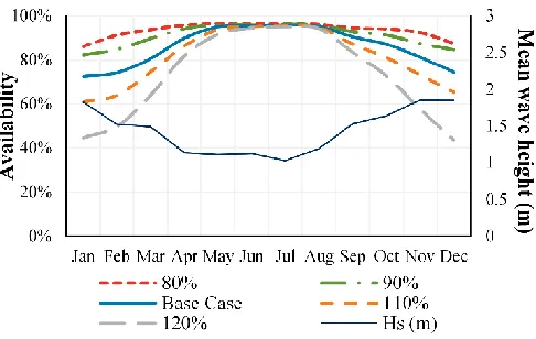
The change in monthly availability (left hand Y-axis) with change in wave height (Hs – right hand

Y-axis) is shown in Fig. 2. It can be seen that there is an inverse relationship where increases in

wave height result in a reduction in availability of the wind farm. This is due to the reduction in

time where the wind farm is accessible in order to perform maintenance. This effect is strongest in

November – March when observed wind speeds are highest. Between May and September Hs is

typically below the maintenance access threshold of 1.5m. Figure 2 shows that O&M planning in

these months will be less critical for availability than in the winter months. Turbines can be

inaccessible for weeks due to lack of suitable weather windows.

Fig. 2. Sensitivity of monthly availability to wave height

showing criticality of winter months due to increased wave height.

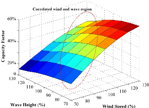
Fig. 3 shows the full range of simulation cases and the joint influence of wind speed and wave

speed and capacity factor and negative correlation between capacity factor and wave height can

be observed. An optimal site would therefore be a site with a benign wave climate but strong wind

climate. However, there is typically a strong, positive relationship between wind speed and wave

height [29] which is identified in Fig. 3. The anticipated correlated region of wind speed and wave

height is also highlighted.

Fig. 3. Impact of wind speed and wave height on capacity factor with the correlated region of wind speed and wave

height highlighted, representing expected operating region.

Due to the positive correlation between wind and wave parameters, it is physically unlikely that

the optimal operational conditions would ever be observed at a real world site. The challenge

therefore is to identify a point at which the gains from increasing wind speed are negated by the

reduction in availability from increased wave height.

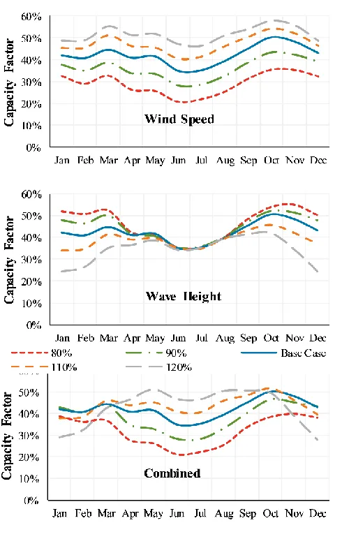
Fig. 4 shows the influence on monthly capacity factors from changing wind speed and wave height

individually and in an associated combination. It can again be seen that there is an increase in

capacity factor from higher wind speeds regardless of time of the year. Conversely, the influence

Fig. 4. Change in capacity factor due to climate identifying importance of considering combined climate

Considering the combined scenario, it can be seen that the reduction in availability associated with

increased wave height negates the benefit from increased wind speed. This results in an optimal

capacity factor value for a given wind farm and accessibility configuration, shown in Fig. 5. For

the baseline scenario a 10% increase in wind speed and wave height values maximizes capacity

factor. Beyond this, the benefit from increased wind resource is cancelled out by reduction in

availability. This is an important result for future site feasibility studies. Sites further from shore

is a reduction in failure repair and maintenance requirements or an improvement in access

technology.

The variability of climate both between sites and between years at a given site are beyond the

control of wind farm and network operators. However, it is possible to negate the negative impact

of increased wave height by increasing the access threshold at which maintenance can be

performed. The monthly improvement in capacity factor for the baseline scenario with increased

access threshold is shown in Fig. 6.

Fig. 5. Individual and combined sensitivity showing combined optimal scenario

The results in Fig. 6 have important consequences for both wind farm and network operators.

Previous analysis of access threshold has focused on overall availability, such as in [2]. This

analysis replicates the observations from these studies and provides additional insights. For wind

farm operators and developers, it is possible to make a more informed financial investment

decision regarding vessels with improved access capabilities or turbines with a track record of high

reliability. The wholesale value of electricity will vary throughout the year depending on the

market that it is being sold into and therefore the full economic case for improved access thresholds

can only be made by considering increase in generation potential rather than availability alone.

For system operators, improved availability from greater accessibility will not result in a uniform

increase in power output throughout the year. This has the possibility to increase the variability

into the wider electricity network and increase the challenge of balancing the system. By

understanding the combined influence of operational climate it will reduce risk to the system that

this variation presents. This analysis clarifies the extent of the challenge and associated costs of

integration into the power network in a new level of detail. Finally, identifying that increased

output from periods of high wind speed may be curtailed by poor accessibility will improve

operational planning.

4. MODELLING INSIGHTS

Through the process of developing the operational model, a number of insights have emerged from

applying such tools in this domain. Through interviews and workshops, data was collected on the

decision maker’s views on applying Monte Carlo simulation models for this problem. Two

First, due to its extensive use, all the engineers were familiar with Monte Carlo simulation and

were comfortable having detailed discussion about aspects of the model such as the underlying

structure of the model, assumptions, boundaries and scope. This made it easy to explore key

aspects of applied modelling such as validation against observed real world performance. Wind

farm planners responsible for CAPEX budgets must be able to show that their key decisions are

rooted in sound engineering assumptions, therefore an ‘open box’ model which can be

interrogated, and its assumptions articulated, is crucial for this application. If an analytical solution

had been sought, it is likely that it’s overly complex mathematical structure would have made it

too challenging for decision makers to fully understand the inner workings of the model and

therefore rejected for use in practice. Additionally, the complexity of the problem and dependency

on operational configuration meant that a single analytical model was not possible and separate

models would have been required for each operational scenario and this would be impractical. As

the goal of the modelling was a pragmatic one of supporting engineers make planning decisions,

verification was an important factor of any model development. Verification here was done by

developing a requisite model [31]. A “model is requisite if its form and content are sufficient to

solve the problem” [31]. Validation is an almost impossible task in many modeling approaches.

For the operational model developed here, due to familiarity of the method, the engineers were

able to thoroughly verify the model through discussions with contextual experts, benchmarking

against similar models and through scenario analysis.

Second, throughout the modelling development process, industrial collaborators continuously

requested added variables and assumptions to the model to ensure the model remained

representative of reality, but which over time increased the computational burden on the model.

example of the associated modelling challenge, additions from a single model iteration doubled

the required time to do 1000 simulations from 2 hours to 4 hours. This increase meant that it was

not possible to do real-time sensitivity analysis on many of the model inputs. To overcome this,

emulators [32] have been developed to ensure the model remains tractable for decision making.

However, due to the highly complex relationship between failure time, repair time, climate,

vessels, etc., it has been challenging to accurately represent the output using an emulator.

Like any maturing industry, the wind farm O&M planning problem is a highly fluid one. An

optimal decision made 6 months ago can be rendered obsolete by changes in market conditions.

Models can be used to hedge against such risks but there are limits to modelling capability that

need to be acknowledged. An example of this is the decision of whether or not to purchase a jack

up vessel for maintenance rather than entering a vessel charter contract. As recently as 2014 many

models would have pointed towards vessel purchase as the optimal solution for lowering O&M

costs, via hedging against extremely high vessel charter rates. However, a change in market

conditions, driven by a large drop in global demand for vessels from the offshore oil and gas sector,

means that a vessel purchase today would be highly sub-optimal. The role of simulation models

as a decision support tool is more relevant than ever in light of uncertainties such as these. A

decision maker needs to understand the limitations, as well as the advantages of any model being

adopted. This only adds to the importance of decision support models being easily interrogated

and articulated, and puts into question models based on ‘black box’ where model details are hidden

from the decision maker.

5. CONCLUSION

This paper has considered the relationship between the operational climate and the generation

relationship to wave height with increased sensitivity in months November - March, whereas

capacity factor shows a joint dependency to wind speed and wave height. Increased wind speed

has a uniformly positive correlation to capacity factor throughout the year, while influence of wave

height is seasonally dependent with little influence on capacity factor in summer months. It has

been identified that an optimal site would maximize wind speed while minimizing wave height

however, this is not representative of the physical nature of wind speed and wave height, which

are positively correlated. Planners therefore must balance the risk of poor accessibility from the

wind and wave climate against the reward of increased production occurring at very high wind

speed sites. The choice of solution ultimately boils down to the risk appetite of the wind farm

owner. A truly optimal solution (eg one which maximized overall project Return on Investment)

could involve novel operational setups, such as a field support vessel being on station for large

parts of the year. The flexible model developed here enables such key operational decisions to be

made in a very informed way.

The paper has considered the role that simulation can play in modelling immature engineering

discipline. Many of the challenges facing emerging engineering problems have similar

characteristics, e.g. lack of detailed information, modelling requirements poorly defined and

evolving, high level of uncertainty, complex problems with multiple interacting factors, dynamic

operating environment which can change the optimal solution, etc. These challenges do not

diminish the usefulness of simulation as an engineering tool for immature industries. However, it

is necessary to recognize the impact of the challenges identified on any modelling approach in

order to minimize their impact on the development and implementation of simulations. This can

be achieved by ensuring the adopted modelling methodology is flexible and that the overall project

REFERENCES

[1] European Wind Energy Association (EWEA), "Wind in power – 2013 European statistics,"

2014.

[2] B. Van, G. J. W. V. Bussel, Bierbooms, and W. A. A. M. Bierbooms, "The DOWEC

Offshore Reference Windfarm: analysis of transportation for operation and maintenance," Wind

Engineering, vol. 27, pp. 381-391, 2003.

[3] Y. Feng, P. J. Tavner, and H. Long, "Early experiences with UK Round 1 offshore wind

farms," Proceedings of the Institution of Civil Engineers - energy., vol. 163, pp. 167-181, 2010.

DOI:10.1680/ener.2010.163.4.167

[4] M. Hofmann, "A Review of Decision Support Models for Offshore Wind Farms with an

Emphasis on Operation and Maintenance Strategies," Wind Engineering, vol. 35, pp. 1-16, 2011.

DOI:10.1260/0309-524X.35.1.1

[5] I. Dinwoodie, O.-E. V. Endrerud, M. Hofmann, R. Martin, and I. Bakken, "Reference

Cases for Verification of Operation and Maintenance Simulation Models for Offshore Wind

Farms," Wind Enginering, vol. 39, pp. 1-14, 2015. DOI:10.1260/0309-524X.39.1.1

[6] Aven, T., Zio, E., Baraldi, P., & Flage, R. (2013). Uncertainty in risk assessment: the representation and treatment of uncertainties by probabilistic and non-probabilistic methods. John Wiley & Sons.

[7] Martin, R, Lazakis, I, Barbouchi, S, Johanning, L. 2016. Sensitivity analysis of offshore wind farm operation and maintenance cost and availability. Renewable Energy, vol. 85, pp. 1226-1236, http://dx.doi.org/10.1016/j.renene.2015.07.078

[8] J. D. Sorensen, "Framework for Risk-based Planning of Operation and Maintenance for

[9] J. Feuchtwang and D. Infield, "Offshore wind turbine maintenance access: a closed-form

probabilistic method for calculating delays caused by sea-state," Wind Energy, vol. 16, pp.

1049-1066, Oct 2013. DOI: 10.1002/we.1539

[10] L. Rademakers, H. Braam, T. Obdam, P. Frohböse, and N. Kruse, "Tools for estimating

operation and maintenance costs of offshore wind farms: state of the art," in EWEC 2008, Brussels,

2008.

[11] M. B. Zaaijer, "DOWEC- Overall cost-modelling of the DOWEC lifecycle in a wind farm,"

TUDelft, Netherlands 2003.

[12] F. Besnard, K. Fischer, and L. B. Tjernberg, "A Model for the Optimization of the

Maintenance Support Organization for Offshore Wind Farms," Sustainable Energy, IEEE

Transactions on, vol. 4, pp. 443-450, 2013. DOI:10.1109/TSTE.2012.2225454

[13] E. Byon and Y. Ding, "Season-Dependent Condition-Based Maintenance for a Wind

Turbine Using a Partially Observed Markov Decision Process," Power Systems, IEEE

Transactions on, vol. 25, pp. 1823-1834, Nov 2010. DOI:10.1109/TPWRS.2010.2043269

[14] Dalgic, Y., Lazakis, I, Dinwoodie, I., McMillan, D., Revie, M. 2015a. Advanced Planning for Offshore Wind Farm Operation and Maintenance Activities, Ocean Engineering, vol. 101, pp. 211-226

[15] Dalgic, Y., Lazakis, I, Dinwoodie, I., McMillan, D., Revie, M., Majumder, Y. 2015b. Cost benefit analysis of mothership concept and investigation of optimum chartering strategy for offshore wind farms, Energy Procedia, vol. 80, pp. 63 – 71

[16] D. C. Hill, D. McMillan, K. R. W. Bell, and D. Infield, "Application of Auto-Regressive

Models to U.K. Wind Speed Data for Power System Impact Studies," Sustainable Energy, IEEE

[17] C. Cunha and C. Guedes Soares, "On the choice of data transformation for modelling time

series of significant wave height," Ocean Engineering, vol. 26, pp. 489-506, 1999. DOI:

10.1016/S0029-8018(98)00014-6

[18] T. Schneider and A. Neumaier, "Algorithm 808: ARfit—A Matlab package for the

estimation of parameters and eigenmodes of multivariate autoregressive models," ACM

Transactions on Mathematical Software (TOMS), vol. 27, pp. 58-65, 2001. DOI:

10.1145/382043.382316

[19] N. B. Negra, O. Holmstrom, B. Bak-Jensen, and P. Sorensen, "Aspects of relevance in

offshore wind farm reliability assessment," Energy Conversion, IEEE Transactions on, vol. 22, pp.

159-166, Mar 2007. DOI: 10.1109/TEC.2006.889610

[20] R. Billinton, Power system reliability evaluation. London: Gordon and Breach, 1970.

[21] F. Castro Sayas and R. N. Allan, "Generation availability assessment of wind farms,"

Generation, Transmission and Distribution, IEEE Proceedings-, vol. 143, pp. 507-518, 1996. DOI:

10.1049/ip-gtd:19960488

[22] Zitrou, A., Bedford, T. and Walls, W. "A model for availability growth with application to

new generation offshore wind farms." Reliability Engineering & System Safety 152 (2016):

83-94.

[23] V. Jinkine and V. Ferdinande, "A method for predicting the added resistance of fast cargo

ships in head waves," International Ship Building Progress, vol. 21, 1973.

[24] W. Van Berlekom, P. Tragardh, and A. Dellhag, "Large tankers-wind coefficients and

[25] v. W. Berlekom, "Wind forces on modern ship forms–effects on performance," Trans. Of

the North East Institute of Engineers and ship Builders, vol. 97, pp. 123-132, 1981.

[26] International Electrotechnical Commission, "Wind turbines - Part 26-1: Time-based

availability for wind turbine generating systems," in IEC/TS 61400-26-1 ed1.0, ed, 2011, p. 53.

[27] T. Burton, Wind energy handbook, 2nd ed. ed. Oxford: Wiley, 2011.

[28] J. Jonkman, "Definition of a 5-MW Reference Wind Turbine for Offshore System

Development," National Renewable Energy Laboratory 9781234110574, 2009.

[29] Fugro GEOS, Wind and wave frequency distributions for sites around the British Isles:

Great Britain, Health and Safety Executive, 2001.

[30] I. Dinwoodie, D. McMillan, M. Revie, Y. Dalgic and I. Lazakis, "Development of a Combined Operational and Strategic Decision Support Model for Offshore Wind," Energy Procedia, vol. 35, pp. 157-166, // 2013. DOI:10.1016/j.egypro.2013.07.169

[31] Phillips, L. D. (1984). “A theory of requisite decision models.” Acta Psychologica 56: 29-48.

[32] Rougier, Jonathan. "Efficient emulators for multivariate deterministic functions." Journal of Computational and Graphical Statistics 17.4 (2008): 827-843.

TABLE I

Baseline wind farm specification

Variable Value Description

Number of Turbines 80 NREL, 5MW [29]

Climate FINO1 100m Met mast in North Sea [31]

Number of vessels 3 Vessel based on Windcat Workboat Mk1

Failure rate 7.5 Categories from [32], failure rates from [7]