Spatially and angularly resolved spectroscopy for in-situ estimation of concentration and particle size in colloidal suspensions

1

Spatially and angularly resolved spectroscopy for in-situ estimation of

concentration and particle size in colloidal suspensions

Yi-Chieh Chen1_{, David Foo}1_{, Nicolau Dehanov}1_{, Suresh N. Thennadil}2*

1_{Department of Chemical and Process Engineering, University of Strathclyde, Glasgow G1 1XJ, UK} 2_{School of Engineering and Information Technology}

Charles Darwin University, Darwin, Northern Territory 0909, Australia *_{Corresponding Author: E-mail: [email protected], Tel: +61 8 89466564}

Graphical Abstract

Graphical Abstract

A probe designed to acquire diffuse reflectance measurements at different source-detector

distances for 3 incidence angles 0

_{, 30}

_{and 45}

_{was used to estimate particle size and}

concentration of polystyrene beads in aqueous suspension using Partial Least Squares

calibration models.

Light

Source

Detector

Calibration model

Particle size

Concentration

Spatial-angular

2

Abstract

Successful implementation of process analytical technology (PAT) hinges on the ability to make continuous or frequent measurements in-line or at-line of critical product attributes such as

composition and particle size, the latter being an important parameter for particulate processes such as suspensions and emulsions. A novel probe-based spatially and angularly-resolved diffuse reflectance measurement (SAR-DRM) system is proposed. This instrument, along with appropriate calibration models, is designed for online monitoring of concentration of chemical species and particle size of the particulate species in process systems involving colloidal suspensions. This measurement system was investigated using polystyrene suspensions of various particle radius and concentration to evaluate its performance in terms of the information obtained from the novel configuration which allows the measurement of a combination of incident light at different angles and collection fibres at different distances from the source fibres. Different strategies of processing and combining the SAR-DRM measurements were considered in terms of the impact on partial least squares (PLS) model performance. The results were compared with those obtained using a bench-top instrument which was used as the reference (off-line) instrument for comparison purposes. The SAR-DRM system showed similar performance to the bench top reference instrument for estimation of particle radius, and outperforms the reference instrument in estimating particle concentration. The investigation shows that the improvement in PLS regression model performance using the SAR-DRM system is related to the extra information captured by the DRM configuration. The differences in SAR-DRM spectra collected by the different collection fibres from different angular source fibres are the dominant reason for the significant improvement in the model performance. The promising results from this study suggest the potential of the SAR-DRM system as an online monitoring tool for processes involving suspensions.

Keywords

3

Introduction

Process spectroscopy is an application of spectroscopic techniques used to analyze a manufactured product or monitor process performance and conditions at-line or in-line, in contrast to the conventional lab-based spectroscopic techniques, to achieve cost effective and timely measurements of process and product related attributes. Near infra-red (NIR), Raman and FTIR are the most widely used techniques for process spectroscopy. NIR spectroscopy has been the major technology segment in process spectroscopy, due to the US Food and Drug Administration's Process Analytical Technology (PAT) initiative in 2004 that seeks to streamline drug manufacturing processes, followed by the EMA’s Guideline on the use of Near Infrared Spectroscopy and the data requirements by the pharmaceutical industry [1, 2]. In addition to the pharmaceutical industry, there is also increasing interest and emphasis from other chemical process industries on in-line monitoring of vital product-related indicators, such as chemical concentration and particle radius, during various process steps. Despite its great potential, significant challenges remain in the successful utilisation of process spectroscopy for analysis of samples/systems containing particulates, such as powder mixture or particle suspensions. The presence of particulates introduces light scattering effect, a light-matter interaction that re-distributes a scattered light non-linearly and increases the diffusiveness of an incident light, depending on physical characteristics of the particulate. It manifests in spectral characteristics by non-linear variation in intensity, shape and baseline. This is a generic phenomenon which affects optical based measurements, and causes uncertainty in the analysis of interference in the measurement which cannot be regularised or mitigated. Diffuse reflectance measurement (DRM) setup is normally used to collect spectra in the wavelength range from UV-vis to NIR from these type of samples. It uses either an integrating sphere for total diffuse reflectance measurement, or a fibre-optic probe placed on the surface of, or inside the sample to collect the signal. The latter approach is usually used for online monitoring of suspensions [3]. In this case, light is delivered by one or more source fibres and the reflected light is collected by several detection fibres. As the technique collects the light after it being scattered and absorbed when travelling through a turbid sample, the DRM spectra contain both absorption and scattering information which can be related to the chemical and physical properties of particulate suspension. The light scattering effect introduces non-linear spectral variations to the pure absorption spectrum of a chemical species, typically manifested as asymmetric absorption peak broadening, nonlinear changes in absorption intensity and spectral baseline. The DRM hence presents limitations on obtaining accurate estimation of chemical and physical information.

Currently, the common approach to reducing the impact of light scattering is by using empirical scatter correction techniques. Various empirical based signal pre-processing methods are commonly used, such as multiplicative scatter correction (MSC) [4], standard normal variates (SNV) [5], extended multiplicative scatter correction (EMSC) [6], first or second derivative of the signal [7] and others [8-10]. The methods are aimed at linearizing the chemical related information or remove spectral variation due to scattering effect and/or other non-chemical effects, returning a pre-processed spectrum which correlates better with the regressand (such as concentration of analyte). In their review, Rinnan et al [11] came to the conclusion that SNV and MSC are the recommended pre-processing methods for scatter-correction in most cases.

4 size [14]. Regression model for the analyte of interest can then be built using Partial Least Squares (PLS) regression or similar methods with potentially better performing models than would be obtained using empirical scatter correction techniques. In order to apply this approach, multiple measurements are required. For in-situ and on-line applications, this can be achieved by collecting light from detection fibres placed at specific distances from the source fibre. This approach is known as spatially resolved diffuse reflectance measurement (SR-DRM). Each SR-DRM spectrum (i.e. spectrum for each detection fibre) corresponds to a different light travelling path in a sample, hence being affected differently by the scattering and absorption effect.

The design of SR-DRM is popular in the application of NIR spectroscopy in the field of biomedical diagnostics where the multiple measurements are used to determine the change in tissue and cell structures and to extract physiological information [15]. The multiple measurements are used to decouple the absorption and scattering effects through the use of radiative transfer theory [16]. Several methods have been developed for inverting SR-DRM spectra to obtain the bulk absorption and scattering spectra. These include the diffusion approximation [17-19] and Monte Carlo combined with interpolation [20-21], multivariate calibration [22] or neural networks [23]. More recently, Watté et al [24] proposed a meta model approach which they investigated using intralipid suspensions over a wide range of concentrations. In all these papers, it is clear that inverting spatially resolved measurements to obtain sufficiently accurate absorption and scattering spectra is very challenging due to the high correlations that exist between the intensities of the spatially distributed detection fibres and the limited number of such fibres that can be used due to the rapid drop-off in signal intensity with distance. As a result, the errors in the extracted absorption and scattering spectra can be considerable. This error will be further propagated when used for extracting particle size and concentration information from the measurements.

Owing to these challenges, to our knowledge, there has been no work in the literature that has sufficiently demonstrated the successful utilisation of the radiative transfer theory with spatially resolved measurements to provide estimates of particle size and concentration of chemical species in a suspension which can surpass the performance of using spectroscopic measurements (such as reflectance and transmittance) in conjunction with chemometrics. It has also not been demonstrated that spatially resolved spectroscopy using chemometrics will provide better results than just using a standard reflectance probe. Off-line measurements using reflectance or transmittance using a research grade laboratory instrument has been widely used and can be considered as the standard against which these new approaches should be tested. Therefore, such measurements will serve as the benchmark for this study.

This problem might be alleviated by introducing new variation in measurement configurations which relates differently to the light scattering characteristics. We propose a novel spatial and angularly resolved diffuse reflectance measurement (SAR-DRM) system which incorporates extra source fibres to deliver light at different incident angles for improving the signal content of the measured spectra. The improved signal content could be beneficial to the calibration models for achieving desired performance and robustness without the necessity to extract the absorption and scattering properties by invoking the computationally intensive radiative transfer theory. In this paper we address the following questions:

5 measurements of each sample compared to using a consolidated value of reflectance where the reflectances from all the fibres are added together as is the case in normal fibre optic reflectance probes.

(2) Will the addition of angularly resolved measurements provide an improvement over the spatially resolved measurements in terms of improved calibration model performance?

If sufficient improvement and robustness of the calibration models can be achieved with this approach then for many cases it may not be necessary to attempt to extract the absorption and scattering spectra by invoking the computationally intensive radiative transfer theory. This paper will investigate these questions using colloidal suspensions drawn from emulsion polymerisation reactions. While the goal is to use this technology platform for online measurements, this initial study focussed on proof-of-concept by carrying out offline measurements so that a controlled dataset spanning a realistic range of conversions (monomer concentrations) and polystyrene particle radiuses and concentrations can be collected so that the questions raised above can be rigorously addressed.

Experimental and Methodology

SAR-DRM Instrument setup

The system for SAR-DRM consists of the following component: a light source using tungsten-halogen lamp, an optical fibre probe with multiple source and detecting fibres, a 16x2 optical multiplexer connected to UV-vis-NIR spectrometers. The system uses N.A. = 0.22, low-OH optical fibres with 200um in diameter. Figure 1(a) shows a schematic drawing of the SAR-DRM setup.

Light source The light source uses a 400W lamp positioned in a modified lamp house (LSH-T100, Horiba Jobin-Yvon) and powered at 29V, 10A. The lamp house couples the light into the source fibres in a ferrule which illuminate the incident light at the end of optical fibre probe. The lamp house also provides a shutter for blocking the incident light entering the optical fibre.

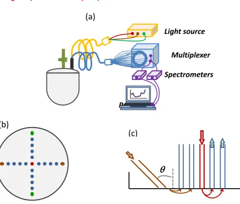
SAR-DRM Probe The custom built, multi-leg SAR-DRM probe used in this study consists of 5 source fibres and uses 16 fibres to collect the diffuse reflectance signal. Black PEEK (Victrex) was used to hold all the fibres at the probe end using black epoxy for adhesion. All fibres are polished to the surface of the probe end. A schematic drawing of the view at the probe end is shown in Figure 1(b) and (c) [25]. The probe offers a maximum of 48 (3 incident angles x 16 fibres) combinations between the source and collecting fibres. However, considering the fibre arrangement, the probe consists of a total of 20 configurations in terms of the spatial and angular relationship between the source and detecting fibres. After data collection it was found that two of the fibres appeared to be damaged judging from the spectra collected from these fibres. Therefore, the analysis presented here is based on data from 14 fibres i.e. 42 (3 incident angles x 14 fibres).

6

Optical Multiplexer and spectrometer The 16 collecting fibres were connected to the 16x2 optical multiplexer (FOM-UVIR200-2x8, Avantes) to couple to 2 optical fibres which connects to the two spectrometers in UV-vis-NIR spectral region (USB4000 and NIRQuest 2.2-512, Ocean Optics). The multiplexer uses a stepping motor to switch between the 16 channels of the incoming signal to couple with the 2 optical fibres for the output channels. The UV-vis-short NIR spectrometer uses 3648 pixels to provide spectral coverage between 350-1000 nm with a ~0.2 nm spectral interval. The NIR spectrometer provides 512 pixels cover spectral range between 900-2100 nm with 4-5 nm data interval. Typical measuring time for the UV-vis-short NIR is 25-100 ms, and 2 s for the NIR spectra. For each sample, the UV-vis-NIR spectrum from each of the 16 collecting fibres was detected individually by scanning across the 16 channels for an incident illumination angle. The same steps were repeated for incident light at all 3 angles, resulting in a total of 48 spectra measured.

Control software The key components (multiplexer and spectrometer) came with own software, however, for the SAR-DRM system an integrated platform was developed in MATLAB (R2012b, Mathwork) utilising the Data Acquisition Toolbox to synchronise the spectra acquisition and the switching of the multiplexer channels. To complete a typical measurement for the total of 48 spectra allowed takes around 5 min.

Materials

The dataset was created by using polystyrene latex suspensions that were available in-house from previously run emulsion polymerisation reactions. Seventeen batches were run by varying the reaction temperature, surfactant concentrations and monomer concentrations and monodisperse polystyrene particle suspensions with radius ranging 50-250 nm were prepared. Materials for the reactions were purchased from Sigma-Aldrich (United Kingdom). Details of the reactions are given elsewhere [26]. Of the seventeen batches, the stock suspensions were chosen from a subset that in general provided a dataset for which the mean particle radius was reasonably evenly spread across the range since many of the batches had similar particle radius. This was to limit the number of samples to be measured (both spectroscopy and reference measurements) to a practical number. These latex suspensions were diluted to obtain different particle concentrations for each particle size. This was done by drawing an aliquot from the sample and diluted to a predetermined value. Each time a separate aliquot was drawn from the sample to ensure that any errors arising from the dilution are independent. In this manner, a samples of polystyrene particle suspensions of various particle radius and concentration were prepared. Particle concentrations of the suspensions covered a range between 2-15% by weight, which were measured gravimetrically as described later. The particle radius was measured using dynamic light scattering (DLS) as described later. Several samples had to be discarded due to issues arising from possible aggregation during storage. After removing outliers due to bad samples possibly due to agglomeration and in some cases malfunction of instrument during measurement, 45 samples were available for the study. The particle radius and concentration for each of the 45 samples are provided in the supplementary materials (Table S1).

Measurements

7 incident illumination is on and off (by using the shutter to block the incident light). All signal collected at this stage are subjected to further signal processing. The SAR-DRM intensity was normalised by using a reference spectrum (𝐼_{𝑆𝑝ℎ𝑒𝑟𝑒}) obtained from a 3.3” integrating sphere (Newport) where the fibre optics probe was fitted into the sphere via an adapter for a 1” port. The same measurement steps used for the samples were followed. It should be noted that the spectra of the diluted samples were measured in random order with respect to their particle diameter and concentrations. This was done to avoid chance correlations due to the order of the measurements affecting the dataset.

Total diffuse transmittance and reflectance measurements Total diffuse transmittance (Td) and reflectance (Rd) were collected from the polystyrene suspensions loaded in a 1 mm path length cuvette using a Cary 5000 (Varian) spectrometer equipped with an external diffuse reflectance accessory (DRA-2500), as the reference spectroscopic measurement. The measurement set up is the same as that used in earlier work [12]. The same sample running order to the SAR-DRM was used, the spectra between 300-2130nm with 1 nm internal were collected using 1 s for the integrating time. Results using the measurements from Cary 5000 were considered as benchmark results.

Dynamic Light Scattering (DLS) measurements Particle radius measurements were obtained using the DLS technique performed by a Nanosizer ZS (Malvern) as the reference method. Due to the DLS measurement requiring particle at concentration that produces single light scattering process, the polystyrene suspensions were diluted by over 1500:1 to bring the concentration within the range of the instrument’s capability. An aliquot of the diluted sample was drawn. Using the built-in parameters to fit the measurement, the estimated mean particle radius was taken from the average radius estimates over 3 runs. These 3 replicates were used to estimate the standard deviation for each measured radius. The overall standard deviation was then calculated as the average over the 45 samples. This was found to be 1.76 nm. For the purpose of comparing the different approaches, the uncertainty in the reference measurement for particle radius is taken to be 2 times the overall standard deviation (= 3.5 nm).

Gravimetric measurements Reference measurements for the particle concentration were obtained separately using gravimetric measurements. 1 ml of the suspensions was placed in a glass vial and dried in an oven at 100 o_{C for 8 hrs, weights of the empty vial, vial containing the samples before and} after the drying were recorded. The actual weight of polystyrene particles was calculated after deducting the weight of surfactant, according to the starting concentration of the surfactant for each reaction, from the remaining solid in the vial for the particle concentration by weight. Three replicate measurements were made for each sample and the overall standard deviation was calculated in the same manner as for radius. The overall standard deviation was 0.11 wt% and the uncertainty in the measurement was taken as 2 times the overall standard deviation (= 0.22 wt%).

Data processing

All data processing were performed using MATLAB (R2012b, Mathworks). Td and Rd spectra from the CARY 5000 spectrometer (benchmark measurements) were smoothed using Savitzky-Golay filter, using the function (‘savgol’) in PLS Toolbox (Eigenvector Research Inc.). The smoothing window size was set to 21 data points (=21 nm) and polynomial order was 2.

8 intensity profile of the light source and the impact of the responses of the optical components on the light reaching the sample, variation of coupling efficiency among the channels of the multiplexer and any other instrument characteristics that will impact the signal received by the detector. This was performed by normalising the spectra from a sample using the spectra collected from the integrating sphere as indicated below.

The first step of the process is to calculate the intensity of the measurement. Dark signal (signal without incident illumination) was subtracted from the signal obtained when the illumination for all 48 source-to-collecting fibre combinations. The subtracted signal was then smoothed using the Savitzky-Golay filter (PLS toolbox by Eigenvector Research Inc.) with a smoothing window of 101 data points (20nm) and polynomial order of 2. The final step of the process is to calculate a normalised reflectance (𝐼_𝑅) by taking the ratio of the smoothed intensity spectra of the sample

(𝐼_{𝑆𝑎𝑚𝑝𝑙𝑒}) to the intensity measurement for the integrating sphere (𝐼_{𝑆𝑝ℎ𝑒𝑟𝑒}) as follows:

𝐼𝑅 = 𝐼_𝐼𝑆𝑎𝑚𝑝𝑙𝑒+𝛿

𝑆𝑝ℎ𝑒𝑟𝑒+𝛿 (1) δ is a small number with respect the maximum intensity which is typically around 200 for 𝐼_{𝑆𝑝ℎ𝑒𝑟𝑒} and > 600 for 𝐼_𝑆𝑎𝑚𝑝𝑙𝑒 that was added to offset the smoothed spectra for avoiding the case of 0 divided by 0. In this study, δ=5 was chosen for all the spectra. Strictly speaking, it is not necessary to include δ in the numerator since, it is only necessary to ensure that the denominator does not have a value of 0 (or very close to 0).

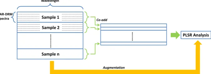
Multi-block Data Sets The SAR-DRM system produces 48 spectra for each sample, corresponding to 20 different spatial and angular configuration for capturing diffuse reflectance signal. The 48 spectra can be regarded as 48 individual data blocks, as well as be combined to produce grouped information, i.e., combining information in multiple data block to produce a final data block for further analysis. There are two approaches to form the final data block, as illustrated in Figure 2.

The first approach co-adds the spectra from the multi-block to form a combined spectrum for a sample. This is similar to many of the probe-based measurement which combines all the returning signal and produce 1 spectrum per sample (excluding replicates). Averaging can be applied to the co-added signal although this is not expected to make a difference in the following multivariate regression analysis. Alternatively, the second approach joins the data blocks by augmentation, forming a large data matrix with the total numbers of variates equal to the sum of the numbers of variates in each individual data blocks. The different approach used to combine the SAR-DRM data might have different effects on the performance of multivariate regression models.

In addition, there are numerous ways data blocks can be formed by varying data blocks selection and combination from the 48 available individual data blocks. For instance, a final data block consisting of spectra of 4 different fibres can be constructed by combining spectra of 4 fibres of the same spatial and angular relationship to the source fibre, or of different spatial and angular relationship. This could also lead to different results in further analysis.

9 selected randomly as test samples. The remaining 36 samples forms the calibration set and the PLSR models were built using leave-one-out cross-validation. The calibration and test data sets were split prior to any data pre-processing steps so the pre-processing parameters determined by the calibration data set were applied to the test set.

It was pointed out by one of the reviewers that the test set may not be independent of the

calibration set given that they are dilutions of samples which are present in the calibration set.

The alternative would be to construct a test set with samples which are drawn from the same

stock solution i.e. all the dilutions from a particular batch. While naturally there will be

correlations between components when a base stock suspension is diluted, here we have a

calibration dataset which was made up of diluting different base stock suspensions obtained

from different batches. For example, a stock suspension with particle radius 50 nm and solids

concentration of 20% by volume with a monomer conversion of 50% (plus some specified

amount surfactant and initiator) is diluted by a different extent than a stock suspension

containing 250 nm an solids concentration of 10% and 70% conversion (different amount of

surfactant and initiator compared to the first example). So correlations across the dataset will

be broken even if the samples within a batch will correlate.

When the dataset is relatively small, the advantage (if any) gained by completely leaving out

entire set of observations which may possibly be correlated is offset by the fact that a “gap” is

created in the particle size. Since the dataset consists of samples with only 6 distinct mean

particle sizes, this can lead to larger uncertainties particularly in the estimation of particle

radius. Further, since this is essentially a comparative study, any effect of correlation can be

expected to equally impact the different approaches and thus any differences in performance

can be attributed to the differences between the approaches. As a check, the analysis was

carried out as follows: Samples from three batches (samples with same particle size and their

dilutions) were taken out to form the independent test set: radius = 107.5, 150.25, 190.75 nm.

Each group had 3 samples (different dilutions). It was found (data not shown) that the

conclusions arrived from way the data was originally split into calibration and test set was not

significantly different from when distinct batches were taken out to form the test set. As

expected, the errors in prediction of particle radius were higher in this case. However, the

relative performances of the different approaches were still similar. Therefore, the results and

discussions will be based on the data set being split as indicated in the first paragraph of this

section.

Three common empirical pre-processing methods, MSC, EMSC and SNV were applied prior to building the PLSR models, and mean centring was applied for all datasets. For the SAR-DRM data sets, if the data from multiple fibres was combined using augmentation approach, the pre-processing was performed on individual data block of the chosen fibre and the resultant pre-processed data blocks for each fibre were augmented to form the final data block. Matlab code for these pre-processing methods were written in-house and used in earlier works [12-14, 27].

10 to the wavelength of the Td and Rd measurements. The final SAR-DRM, Td and Rd data sets contain the same spectral range (450-900nm) and interval (1 nm) for the regression analysis. Data set formed using the co-adding approach will therefore have the same wavelength intervals in the data matrix as Td and Rd data sets. This eliminates the effect of the numbers of variables on the PLS regression model performance.

The number of latent variables was chosen based on leave-one-out cross-validation and inspecting the curve of root mean square error of cross-validation (RMSECV) vs number of latent variables (LV). The value of LV which provided the lowest RMSECV was chosen if this was a clear minimum value. In many cases the RMSECV curve has a relatively flat profile after appreciable drop in value in the first few latent variables. In this case, a lower LV which was chosen based on visual inspection of the curve so that the RMSECV of higher LV models give negligible reduction in RMSECV. For cases where RMSECV decrease monotonically with an apparent flat profile, a model using no less than 6 LV was chosen, after visual inspection of loading curves of the higher LV. The minimum of 6 LVs is decided based on the numbers of varying component in each sample (particle size, particle size distribution, concentration of particle, water, surfactant and residual styrene). The choice of using the number of LVs above 6 is based on both the decrease in the RMSECV and visual examination of the loadings of those LVs. For example, if the RMSECV is decreasing continuously up to number of LVs equal to 10 but loading for LVs from 9 is noisy, then the number of LVs is chosen to be 8 i.e. up to the LV which shows systematic behaviour. It should be noted that, for each iteration of the leave-one-out cross-validation, the spectra were mean-centred by using the mean spectrum which does not include the left-out spectrum. Once the best calibration model for each input data set was chosen, model comparison was made based on the RMS error of cross-validation (RMSECV) and in predicting the test samples (RMSEP).

Results and Discussions

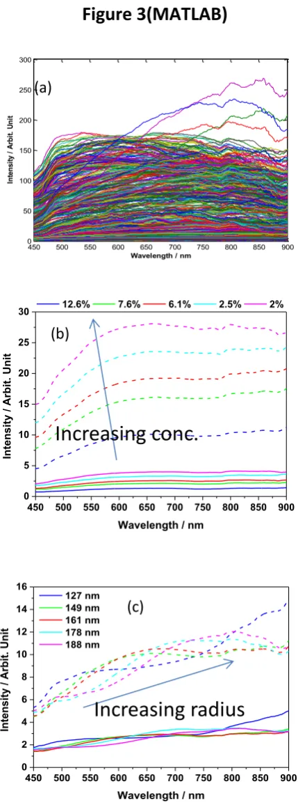
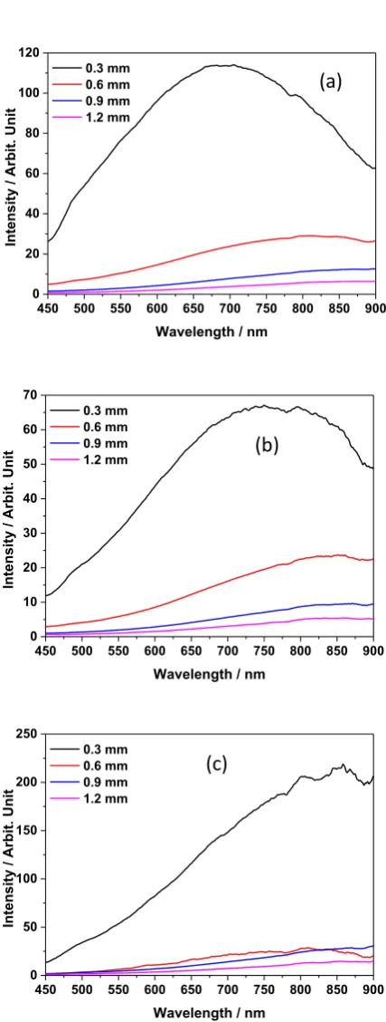
SAR-DRM spectra from the polystyrene suspensions using all 48 source-detecting fibre combinations are shown in Figure 3(a). Figure 3(b) and (c) shows examples of changes in spectra from different source-detecting fibre distances for samples of similar particle radius with varying concentration, and those of similar concentration with varying particle radius. Figure 3(b) shows that the decrease in intensity with increasing concentration is dependent on the wavelength. At wavelength of 450 nm the intensity increases by about 3 times from the highest to the lowest concentration, but this is only about 2.5 times at wavelength of 900 nm. In Figure 3(c), the wavy pattern of the spectra shifts toward longer wavelength as the radius increases, without appreciable systematic changes in magnitude. The non-linearity of the spectral variations with concentration is a characteristic of light scattering effect and commonly observed in NIRS study of turbid media. In addition, increasing the distances between source-detecting fibres decreases non-linearly the intensity. For example, an intensity ratio between the two fibre distances of around 4.4 is obtained at wavelength of 450 nm, but the ratio increases to around 8 at wavelength of 950 nm. The rationale behind the observation is simple; the optical path for light to travel through the sample and reach a detecting fibre varies with different source-detecting distances, hence the spectra manifest differently the non-linear light scattering effect.

11 intensity differences between fibre distances are evident. By changing the angular relationship between the source and collecting fibres, diffuse reflectance at a specific angle is captured to provide angular-resolution of the total reflectance from a sample of specific set of scattering and absorption properties. For a uni-directional incident light, the diffusiveness of the light increases as it undergoes light scattering event, i.e., the angular distribution of the scattered light varies as the incident light travel into a light scattering medium, and the longer it travels the more diffusive the light becomes. The design of SAR-DRM configurations facilitates angular measurement configurations in order to obtain a more complete profile of the light scattering properties which could relate to physical properties of the scatterers. Figures 3 and 4 indicate the complexity in the information associated with each source-detecting fibre distances; it is not interpretable by a simple multiplicative effect.

The results are organised into two parts. Part One comprises comparisons of the SAR-DRM performance to the reference spectroscopic measurements (i.e. using the CARY 5000 spectrometer) for estimating physical (particle radius) and chemical (particle concentration) characteristics of the polystyrene suspensions. Part Two investigates further the source of information contained in the SAR-DRM spectra that affects the model performance. It examines changes in the model performance for particle radius and concentration estimation by changing the amount of spectra used to construct the data sets.

Part One – Estimation of Particle Radius and Concentration

To determine the usefulness of the angular configuration provided by SAR-DRM, we compare the regression models built on the SAR-DRM spectra, with benchmark models built using the total diffuse transmittance and reflectance measured by the reference spectrometer, CARY 5000 (spectra shown in supplementary material, Fig S1). The SAR-DRM spectra collected from all 48 fibre combinations are organised into two data sets for using the data co-adding and augmentation approaches. The data co-adding approach imitates the signal provided by conventional reflectance measurement probes. It returns a single-block data set with a combined reflectance for each sample. The augmentation approaches re-arrange the 48 spectra from a sample, resulting in a long array containing 18542 (= 42*451) variables for each sample.

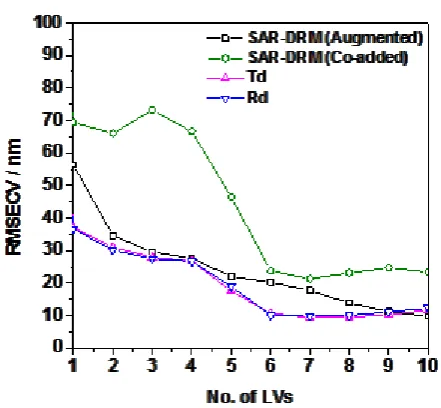
A clear difference in the calibration model performance is seen in Figure 5 between models built on the spectra using co-adding and augmentation approaches for estimating particle radius. At this stage, no data pre-processing step was applied. As stated earlier, the SAR-DRM data set arranged using the co-adding approach mimics the spectra normally obtained from reflectance probes. In this case, the model results in higher RMSECV values, especially when only using small numbers of LVs are used. The same SAR-DRM spectra, when combined using the augmentation approach, result in a smoother LVs curve with the overall REMSECV level similar to the model built on the spectra (Td and Rd) from the reference spectroscopic instrument. In addition, it is also seen that the LV curves for models built on Rd and Td exhibit similar results. This could be due to the negative correlation between the two measurement configurations in a spectral region dominated by the light scattering effect. The sum of the measured Td and Rd from a purely scattering media should be equal to 1 as there is no loss of light due to absorption (and assuming other light-matter interactions are negligible). Td and Rd respond to changes in sample condition in a similar way (but in opposite direction in terms of its intensity), hence result in similar model performance.

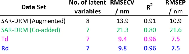
12 Model performances are summarized in Table 1. Noting that the uncertainty in the reference values is 3.5 nm, it can be seen that a significant drop in RMSEP is achieved by using augmentation (10.9 nm) instead of co-adding (21.6 nm). Both are higher compared to the benchmark measurements. However, the difference in RMSEP between the model based on augmented data and the models based on benchmark data is within the experimental uncertainty of the reference values. Examining the prediction plot (Estimated vs. Actual), it was found that for the SAR-DRM data set using the co-adding approach (Fig. S2(b) in supplementary material) appears to lead to increased uncertainty in the estimated particle radius near the boundaries of the particle radius range compared to the other models (Fig. S2(a), (c) and (d)).

The number of latent variables chosen for the models is high for all the cases. As explained earlier, there are 6 possible components in the system that can vary though the major variations will be due to variations in particle size and concentration. It was felt that this number was justified due to the fact that the latent variables did not appear to be noisy until about LV 9. This can be seen from Figure S3 in the supplementary material where the loadings plots for the augmented dataset corresponding to the results shown in the first row of Table 1 are provided.

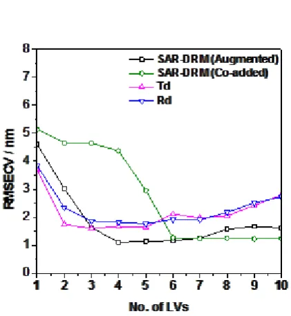
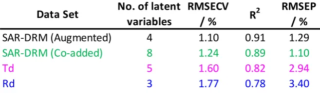
Similar analysis of calibration model performance was also conducted with the model for estimating particle concentration. Figure 6 and Table 2 show that the models built on SAR-DRM data sets outperform those built using the benchmark Td or Rd measurements. The RMSECV curves for the models built with Td and Rd exhibit similar shape due to the same reasons as was discussed previously, for models built to estimate particle radius. The cross-validation error in the estimated particle concentration is slightly lower (see Table 2) when using the augmented dataset compared to the other 3 approaches, but given that the reference value has an uncertainty of 0.22 wt%, this improvement does not appear to be statistically significant. The RMSEP, on the other hand, indicates that the SAR-DRM with augmented data can outperform the benchtop measurements. Based on the combined observation of the RMSECV and RMSEP, the SAR-DRM may have the potential to outperform the bench-top measurements. Also, the number of latent variables required for the augmented dataset is 4 while, it is double that for the co-added dataset. This indicates that a large gain in model parsimony can be achieved using augmentation. The prediction plots (Estimated vs Actual concentration) are given in supplementary materials (Fig. S4).

Part Two - Why better models performance from the augmented data set?

The PLS regression analysis in Part One indicated interesting results that, although using the same SAR-DRM spectra to build the data set, the model performance on the physical and chemical characteristics is dependent on the data combining strategy. As the co-adding approach represents the way that DRM signals are typically captured and produced by a reflectance probe, it is important to investigate the cause of the superiority of the model performance. There are three possible hypotheses to explain the observed phenomena:

(1) The augmented data set provides significantly more variables than the co-adding approach. Those additional variates are treated as extra information for the PLS regression model to improve the accuracy of estimation.

13 spectra by co-adding these differences would lose those distinct differences, and deteriorates the model performance.

(3) The inclusion of angular incidence provides extra information that can be utilised by regression models

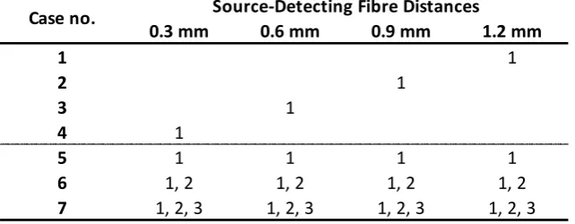
To investigate these possibilities, PLS regression analysis was applied to a number of data sets created by different combinations of source-detecting fibre configurations available. There are 7 cases based on different combinations that were studied.

Cases 1-4 used measurements from only 1 source-detector distances namely 1.2 mm, 0.9 mm, 0.6 mm and 0.3 mm respectively. These cases were studied to determine whether there is a significant impact in the way measurements from multiple fibres with the same source-detector distance are combined together, i.e. whether there is a difference in augmentation and co-adding approach. Since there are multiple detection fibres for each source-detector distance, they were used to examine this aspect for each of the 4 available source-detector distances. Note that only the measurements where incident light is normal i.e. angle of source fibre is 00 _{to the normal is considered in these four cases.}

Case 5 examines the impact of including all the different source-detector distances either by augmentation or by co-adding. In this case, there are 4 source-distance combinations that are considered together. The purpose of investigating Case 5 is to see if introducing different information contained in the different source-detector distances has an impact on the calibration model performance. Also it allows us to examine whether the way this information is introduced i.e. whether augmentation or co-adding is used will affect model performance.

Case 6 is an extension of Case 5 whereby additional measurements using angularly incident light (300 to the normal) are added to the dataset. Thus 8 combinations of source-detector (4 for each incident angle) are considered together.

Case 7 further adds measurements using angularly incident light (450 _{to the normal) to Case 6 so that} 12 source-detector combinations are included in the dataset. The last 2 cases examine whether there is additional advantage in adding angularly incident measurements. Table 3 summarises the seven cases considered in this study. At this stage, no data pre-processing step was applied to the resultant data sets in order to compare directly to results in Part One.

14 co-added data set. Therefore, improvement in the calibration model performance is not simply related to the increase of variables as suggested in hypothesis (1) given above. Co-adding spectra is commonly used to improve the signal-to-noise ratio which subsequently improves model performance. The results suggest that this effect on SAR-DRM data is probably negligible, compared to other factors discussed later in this section.

Tables 6 and 7 summarise the results obtained for estimation of particle radius and concentration respectively. The corresponding RMSECV curves are shown in Fig. S6(a) and (b) in supplementary materials. Comparing, results shown in Tables 4 and 6, it can be seen that if all the source-detector information is used together using augmentation, there is a significant improvement in model performance for estimating particle radius. The lowest RMSEP value obtained when only measurements from one source-detector distance are used is 34.4 nm (Table 4 Case 1). The lowest RMSEP when the different source-detector distances are used via augmentation is 9 nm (Table 6, Case 5). Since the uncertainty reference value of 3.5 nm is much smaller than the difference between these two RMSEPs, the results suggest there is a significant advantage in using the augmentation approach utilising different source-detector distances. However, the addition of extra measurements through different incident angles does not seem to provide additional improvement. The co-adding approach appears to benefit from adding both source-detector and angular measurements with the lowest RMSEP of 21.6 nm (Table 6 Case 7). While this is significantly smaller than when only one source-detector measurement is utilised, it is appreciably higher than the values obtained using augmentation.

For estimation of particle concentration, comparison of Tables 5 and 7 suggests that the adding spatial and angular measurements leads to a slight reduction in the RMSEP which may not be significant compared to the reference value uncertainty of 0.22 wt%. The lowest RMSEP obtained when using a single source-detector distance is 1.52 wt% (Table 5 Case 2) while the lowest RMSEP is 1.29 wt% (Table 7 Case 7) when augmentation, which includes both angular and spatial measurements, is used. However, compared to co-adding the measurements, which gives an RMSEP of 1.1 wt% (Table 7 Case 7), this is not significantly different. Thus, for particle concentration estimation, model performance in terms RMSEP does not benefit from adding extra measurements from different source-detector distances. However, the additional measurements lead to an appreciable reduction in the number of latent variables needed (4 for Augmented and 7-8 for Co-added data), thus leading to a much more parsimonious model when augmented data is used. While the addition of angular incidence measurements gave the lowest RMSEP, there is not sufficient evidence to suggest that they provide an improvement over just using the normal incidence measurements.

Finally, we examine if calibration model performance can be improved for Cases 1-7 by the use of data pre-processing. The concept of data pre-processing is to pre-condition the spectra obtained using the same configuration, typically by removing its slope and baseline variation (such as MSC and EMSC) as well as by regularising the scaling of the spectra (such as SNV). For augmented data sets, the pre-processing step was applied to each configuration separately to preserve the different information captured by the different configurations. For the co-added data sets, the pre-processing was applied following the co-adding step. As mentioned earlier, SNV, MSC and EMSC methods were the scatter correction techniques that were considered.

15 examination of Table 8(a) indicates that even though SNV gives the lowest RMSEP (8.4 nm), taking into account the error in the reference values and RMSECV, it is not clear that this reduction in error is significant compared to MSC or when no pre-processing is applied. However, the model obtained using SNV corrected spectra lead to an appreciable reduction in the number of LVs needed in the model. This indicates that a more parsimonious model can be achieved by using SNV with augmented spectra. Co-added spectra on the other hand, do not indicate any improvement in the RMSEP or for improving model parsimony.

For the estimation of particle concentration, examination of Table 8(b) suggests that there is no significant improvement in prediction error due to pre-processing the augmented spectral data. However, in this case, it appears that not using pre-processing could lead to more parsimonious model. For co-added spectra, it appears that using EMSC could provide a lower prediction error compared to not using any pre-processing. But given that the RMSECV for EMSC is higher than the other methods, it is not clear whether this improvement is significant.

Conclusions

We have presented the design, setup and analysis of a novel probe-based spatially and angularly-resolved diffuse reflectance measurement (SAR-DRM) system. The new system was investigated using polystyrene suspensions of various particle radius and concentration to evaluate the performance of the system in terms of the information obtained from the novel SAR-DRM configuration. This system showed similar performance to the bench top reference instrument for estimation of particle radius, and could have the potential outperform it for estimation of particle concentration. The investigation shows that the improvement in PLS regression model performance using the SAR-DRM system is related to the extra information captured by the SAR-DRM configuration. The study indicates that the extra information is better utilised when the dataset is built by augmentation instead of co-adding the spectra. The increase in signal-to-noise by co-adding additional signal from fibre of the same spatial and angular relationship has negligible effect on model performance except in the case where EMSC is used for pre-processing. However, the conflicting indications given by RMSECV and RMSEP make this improvement suspect.

While the estimation error for particle concentration does not show a significant improvement due to the additional measurements, a more parsimonious model is obtained if the additional spatial measurements are used. Measurements from additional angular incidences seem to improve models in some cases but the improvement is not sufficient to indicate that it is statistically significant for the system studied here. The superiority in the performance from the SAR-DRM system can be concluded to be the result of integrating the novel design of measurement configuration with the data combining strategy i.e. augmentation. The promising results from this study suggest the potential of the SAR-DRM system as an online monitoring tool for processes involving suspensions.

Acknowledgements

16

Declaration of Conflict of Interest

The authors declare no conflict of interest.

References

1. Administration, U.S.F.a.D., Guidance for Industry PAT — A Framework for Innovative Pharmaceutical Development, Manufacturing, and Quality Assurance. 2004: Rockville, MD. 2. Agency, E.M., Guideline on the use of near infrared spectroscopy by the pharmaceutical industry

and the data requirements for new submissions and variations. 2014: London, UK.

3. De Beer, T., Burggraeve A., Fonteyne, M., Saerens, L., Remon, J. P., Vervaet, C. Near infrared and Raman spectroscopy for the in-process monitoring of pharmaceutical production processes.

Int. J. Pharm., 2011. 417(1–2): p. 32-47.

4. Geladi, P., MacDougall, D., Martens, H. Linearization and Scatter-Correction for Near-Infrared Reflectance Spectra of Meat. Appl. Spectrosc., 1985. 39: p. 491-500.

5. Barnes, R.J., Dhanoa, M. S., Lister, S. J. Standard Normal Variate Transformation and De-trending of Near-Infrared Diffuse Reflectance Spectra. Appl. Spectrosc., 1989. 43: p. 772-777. 6. Martens, H., Nielsen, J.P., Engelsen, S. B.Light Scattering and Light Absorbance Separated by

Extended Multiplicative Signal Correction Application to Near-Infrared Transmission Analysis of Powder Mixtures. Anal. Chem., 2003. 75: p. 394-404.

7. Norris, K. H., Williams, P.C. Optimization of mathematical treatments of raw near-infrared signal in the measurement of protein in hard red spring meat. 1. Influence of particle size. Cereal Chem., 1984. 61(12): p. 158-165.

8. Pedersen, D. J., Martens, H., Nielsen, J.P., Engelsen, S. B. Near-Infrared Absorption and Scattering Separated by Extended Inverted Signal Correction (EISC): Analysis of Near-Infrared Transmittance Spectra of Single Wheat Seeds. Appl. Spectrosc., 2002. 56: p. 1206-1214. 9. Svensson, O., Kourti, T., MacGregor, J.F. An investigation of orthogonal signal correction

algorithms and their characteristics. J. Chemom., 2002. 16: 176-188.

10. Chen, Z.-P, Morris, J., Martin E. "Extracting Chemical Information from Spectral Data with Multiplicative Light Scattering Effects by Optical Path-Length Estimation and Correction". Anal. Chem. 2006. 78(22):7674-7681.

11. Rinnan, A., Berg, F.v.d., Engelsen, S. B. Review of the most common pre-processing techniques for near-infrared spectra. Trends Anal. Chem., 2009. 28(10): p. 1201-1222.

12. Steponavicius, R. and S.N. Thennadil, Extraction of Chemical Information of Suspensions Using Radiative Transfer Theory to Remove Multiple Scattering Effects: Application to a Model Two-Component System. Anal. Chem., 2009. 81(18): p. 7713-7723.

17 14. Steponavicius R, Thennadil SN. Full correction of scattering effects by using the Radiative

Transfer Theory for improved quantitative analysis of absorbing species in suspensions. Appl. Spectrosc. 67(5) 526 – 535 (2013).

15. Utzinger, U., Richards-Kortum, R.R. Fiber optic probes for biomedical optical spectroscopy. J. Biomed. Opt., 2003. 8(1): p. 121-147.

16. Doornbos, R.M.P., Lang, R., Aalders, M.C., Cross, M. W., Sterenborg, H. J. The determination of in vivo human tissue optical properties and absolute chromophore concentrations using spatially resolved steady-state diffuse reflectance spectroscopy. Phys. Med. Biol., 1999. 44(4): 967 - 981. 17. Groenhuis, R.A.J., Ferwerda, H.A., Ten, J.J. Scattering and absorption of turbid materials

determined from reflection measurements. 1: Theory. Appl. Opt., 1983. 22 (16):. p. 2456-2462. 18. Groenhuis, R.A.J., Ferwerda, H.A., and Ten, J.J. Scattering and absorption of turbid materials

determined from reflection measurements. 2: Measuring method and calibration.: Appl. Opt., 1983. 22(16): p. 2463-2467.

19. Farrell, T.J., Patterson, M.S. A diffusion theory model of spatially resolved, steady-state diffuse reflectance for the noninvasive determination of tissue optical properties in vivo. Med. Phys., 1992. 19: p.879-888.

20. Dam, J.S., Dalgaard, T., Fabricius, P. E., Andersson-Engels, S. Multiple polynomial regression method for determination of biomedical optical properties from integrating sphere measurements. Appl. Opt., 2000. 39(7): p. 1202-1209.

21. Thueler, P., Charvet, I., Bevilacqua, F., St Ghislain, M., Ory, G., Marquet, P., Meda, P., Vermeulen, B., Depeursinge C. In vivo endoscopic tissue diagnostics based on spectroscopic absorption, scattering, and phase function properties. J. Biomed. Opt., 2003. 8(3): p. 495-503. 22. Farrell, T. J., Wilson, B.C., Patterson, M.S. The use of a neural network to determine tissue

optical properties from spatially resolved diffuse reflectance measurements. Phys. Med. Biol., 1992. 37 (12): p. 2281-2286.

23. Dam, J.S., Andersen, P.E., Dalgaard, T., Fabricius, P. E. Determination of tissue optical properties from diffuse reflectance profiles by multivariate calibration. Appl. Opt., 1998. 37 (4): p. 772-778. 24. Watté, R., Aernouts, B., Van Beers, R., Saeys W. Robust metamodel-based inverse estimation of

bulk optical properties of turbid media from spatially resolved diffuse reflectance measurements. Opt. Mat. Exp., 2015. 5(11): p. 27880- 27898.

25. Thennadil, S.N., Chen, Y. -C. Measurement apparatus and method with variable path lengths and variable reflective surfaces. Patent Application, GB2496690. Date of Filing, 21/11/2011.

26. Dehanov, N., Thennadil, S. N., Monitoring of mean particle size during emulsion polymerisation reactions using visible and near infrared diffuse reflectance spectroscopy. Asia Pacific Conf. Chem. Eng. Cong. 2015 (APCChE 2015) incorporating CHEMECA 2015 / IChemE; EA. ISBN 9781922107473. Library Australia ID 54817420.

18

Figure 1(Microsoft Powerpoint)

Fig. 1 Schematic drawing reproduced from [26] (a) SAR-DRM system. (b) Source and detecting fibre arrangements viewed from the probe end. All detecting fibres are in blue. The red, brown and green solid circles are the source fibres illuminating light from 0, 30 and 45o _{to the probe axis. (c) Definition}

of angle () for the source fibres in (b).

Light source

Multiplexer

Spectrometers

P

C

(a)



(b)

19

Figure 2(Microsoft Powerpoint)

Fig. 2: Illustration of co-adding and augmentation methods for combining SAR-DRM spectra.

……

...…

Sample n

SAR-DRM

spectra Sample 1

Sample 2

Wavelength

…..…

Co-add

PLSR Analysis

20

Figure 3(MATLAB)

Fig. 3 (a) All SAR-DRM spectra collected from the 45 polystyrene particle suspensions. (b) Changes of SAR-DRM spectra for particles of radius 149nm at different particle concentrations (12.6-2%) using fibres of distances of 0.6 (dash lines) and 1.2 (solid lines) mm from the normal incident source fibres. (c) Changes of SAR-DRM spectra for12.6% latex suspensions with different particle radius (127-188 nm) from fibres of distances of 0.6 (dotted-dash lines) and 0.9 (solid lines) mm to the normal incident fibres.

450 500 550 600 650 700 750 800 850 900 0 50 100 150 200 250 300

Wavelength / nm

In te ns ity / A rb it. U ni t

450 500 550 600 650 700 750 800 850 900

0 5 10 15 20 25 30 Intensit y / Arbit. Unit

Wavelength / nm

12.6% 7.6% 6.1% 2.5% 2%

450 500 550 600 650 700 750 800 850 900

0 2 4 6 8 10 12 14 16 Intensit y / Arbit. Unit

Wavelength / nm

21

Figure 4 (MATLAB)

Fig. 4 SAR-DRM spectra of suspension with particle radius of 81 nm and concentration of 12.9% from fibres of 4 different distances to the source fibres at angle  of (a) 0, (b) 30, and (c) 45o

450 500 550 600 650 700 750 800 850 900

0 20 40 60 80 100 120

Intensit

y /

Arbit.

Unit

0.3 mm 0.6 mm 0.9 mm 1.2 mm

Wavelength / nm

450 500 550 600 650 700 750 800 850 900

0 10 20 30 40 50 60 70

Intensit

y /

Arbit.

Unit

Wavelength / nm

0.3 mm 0.6 mm 0.9 mm 1.2 mm

450 500 550 600 650 700 750 800 850 900

0 50 100 150 200 250

Intensit

y /

Arbit.

Unit

0.3 mm 0.6 mm 0.9 mm 1.2 mm

Wavelength / nm

(a)

(b)

22

Figure 5(Origin)

23

Figure 6(Origin)

24

Table 1

Table 1: Summary of calibration model performance for estimating particle radius using different data sets.

Data Set

No. of latent

variables

RMSECV

/ nm

R

2

RMSEP

/ nm

SAR-DRM (Augmented)

8

13.9

0.91

10.9

SAR-DRM (Co-added)

7

21.3

0.80

21.6

Td

7

9.4

0.96

7.5

25

Table 2

Table 2: Summary of calibration model performance for estimating particle concentration using different data sets. Particle concentrations are expressed as % weight of sample.

Data Set

No. of latent

variables

RMSECV

/ %

R

2

RMSEP

/ %

SAR-DRM (Augmented)

4

1.10

0.91

1.29

SAR-DRM (Co-added)

8

1.24

0.89

1.10

Td

5

1.60

0.82

2.94

26

Table 3

Table 3: Measurements configurations on which datasets used for cases 1-7 were built. These were constructed using spectra from collecting fibres of different distances and source fibres of different angles (1 for source fibre of  = 0 o_{, 2 for source fibres of}  _{= 30} o_{, and 3 for source fibres of}  _{= 45}o₎

0.3 mm 0.6 mm 0.9 mm 1.2 mm

1 1

2 1

3 1

4 1

5 1 1 1 1

6 1, 2 1, 2 1, 2 1, 2

27

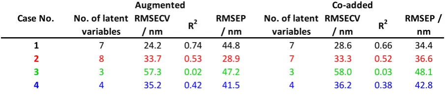
Table 4

Table 4: Summary of calibration model performances for estimating particle radius using datasets from Cases 1-4 with augmentation and co-adding approaches for utilising the data.

No. of latent variables

RMSECV / nm R

2 RMSEP / nm

No. of latent variables

RMSECV / nm R

2 RMSEP / nm

1 7 24.2 0.74 44.8 7 28.6 0.66 34.4

2 8 33.7 0.53 28.9 7 33.3 0.52 36.6

3 3 57.3 0.02 47.2 3 58.0 0.03 48.1

4 4 35.2 0.42 41.5 4 36.2 0.38 42.8

Augmented Co-added

28

Table 5

Table 5: Summary of calibration model performance for estimating particle concentration using datasets from Cases 1-4 with augmentation and co-adding approaches for utilising the data.

No. of latent variables

RMSECV

/ % R

2 RMSEP / %

No. of latent variables

RMSECV

/ % R

2 RMSEP / %

1 7 1.26 0.89 2.01 6 1.34 0.87 1.16

2 8 1.58 0.83 1.52 7 1.45 0.85 1.42

3 8 1.10 0.92 1.68 8 1.32 0.87 1.10

4 3 1.79 0.78 3.01 3 1.87 0.76 3.10

Augmented Co-added

29

Table 6

Table 6: Summary of calibration model performance for estimating particle radius using datasets from Cases 5-7 with augmentation and co-adding approaches for utilising the data.

No. of latent variables

RMSECV / nm R

2 RMSEP / nm

No. of latent variables

RMSECV / nm R

2 RMSEP / nm

5 8 13.3 0.92 9.0 10 35.4 0.47 29.8

6 8 11.4 0.94 12.9 7 27.0 0.68 28.8

7 8 13.9 0.91 10.9 7 21.3 0.80 21.6

Augmented Co-added

30

Table 7

Table 7: Summary of calibration model performance for estimating particle concentration using datasets from Cases 5-7 with augmentation and co-adding approaches for utilising the data.

No. of latent variables

RMSECV

/ % R

2 RMSEP / %

No. of latent variables

RMSECV

/ % R

2 RMSEP / %

5 4 1.24 0.89 1.78 7 1.29 0.88 1.30

6 4 1.19 0.90 1.51 8 1.28 0.89 1.33

7 4 1.10 0.91 1.29 8 1.24 0.89 1.10

Case No.

31

Table 8

Table 8: Summary of calibration model performances when pre-processing was applied to datasets from Cases 1-7. For each pre-processing method (MSC, EMSC, SNV) used, the combination of configurations i.e. the Case for which they resulted in the lowest RMSEP are presented for augmentation and co-adding approach; (a) Estimation of particle radius, (b) Estimation of particle concentration.

(a)

Case No.

No. of latent variables

RMSECV

/ nm R

2 RMSEP /

nm

Case No.

No. of latent variables

RMSECV

/ nm R

2 RMSEP /

nm

None 6 8 11.4 0.94 12.9 7 7 21.3 0.80 21.6

MSC 5 7 16.8 0.87 12.0 7 6 22.5 0.77 23.1

EMSC 3 7 37.5 0.41 61.2 7 6 30.3 0.58 29.3

SNV 6 5 12.2 0.93 8.4 7 6 24.8 0.73 25.2

(b)

Case No.

No. of latent variables

RMSECV

/ % R

2 RMSEP /

%

Case No.

No. of latent variables

RMSECV

/ % R

2 RMSEP /

%

None 6 4 1.19 0.90 1.51 5 7 1.29 0.88 1.30

MSC 5 7 1.24 0.89 1.22 5 7 1.20 0.90 0.86

EMSC 4 8 1.43 0.86 1.35 7 6 1.45 0.85 0.59

SNV 5 7 1.25 0.89 1.42 5 7 1.13 0.91 0.96

Preprocessing Method

Augmented Co-added

Preprocessing Method

32

SUPPLEMENTARY MATERIAL

Figure S1(MATLAB)

Fig. S1 (a) Total diffuse reflectance and (b) total diffuse transmittance of all 45 polystyrene suspensions measured using CARY 5000 spectrometer which was used as the benchmark.

450 500 550 600 650 700 750 800 850 900 0 5 10 15 20 25 30 35 40 45

Wavelength / nm

To ta l di ff us e t ra ns m it ta nc e / %

450 500 550 600 650 700 750 800 850 900 45 50 55 60 65 70 75 80 85 90 95

Wavelength / nm

33 Supplementary Material: Figure S2 (Origin)

Fig. S2. Particle radius prediction plots for SAR-DRM by (a) augmentation, (b) co-adding, and for (c) Td, and (d )Rd.

50 100 150 200 250

50 100 150 200

250 Calibration_Test

Estimat ed radi us / n m

Actual radius / nm

50 100 150 200 250

50 100 150 200

250 Calibration_Test

Actual radius / nm

Estimat ed radi us / n m

50 100 150 200 250

50 100 150 200 250

Actual radius / nm

Estimat ed radi us / n m Calibration Test

50 100 150 200 250

50 100 150 200

250 Calibration_Test

Estimat ed radi us / n m

Actual radius / nm

(a)

(b)

(c)

(d)

LV = 8; R2 = 0.91 RMSECV = 13.9 nm RMSEP = 10.9 nm

LV = 7; R2 = 0.96 RMSECV = 9.4 nm RMSEP = 7.5 nm

LV = 7; R2 = 0.8 RMSECV = 21.3 nm RMSEP = 21.6 nm

34

Supplementary Material Figure S3 (Origin)

Fig. S3. Particle concentration prediction plots for SAR-DRM by (a) augmentation, (b) co-adding, and for (c) Td, and (d) Rd.

0 2 4 6 8 10 12 14 16

0 2 4 6 8 10 12 14 16

Actual conc. / %

Calibration Test Estimat ed co nc . / %

0 2 4 6 8 10 12 14 16

2 4 6 8 10 12 14 16 Calibration Test

Actual conc. / %

Estimat ed co nc . / %

-2 0 2 4 6 8 10 12 14 16 -2 0 2 4 6 8 10 12 14 16

Actual conc. / %

Estimat ed co nc . / % Calibration Test

-4 -2 0 2 4 6 8 10 12 14 16 -4 -2 0 2 4 6 8 10 12 14 16

Actual conc. / %

Estimat ed co nc . / % Calibration Test

(a)

(b)

(c)

(d)

LV = 4; R2 = 0.91 RMSECV = 1.10 % RMSEP = 1.29 %

LV = 5; R2 = 0.82 RMSECV = 1.60 % RMSEP = 2.94 %

LV = 8; R2 = 0.89 RMSECV = 1.24 % RMSEP = 1.10 %

35

Supplementary Material Figure S4 (Origin)

Fig. S4. PLS Loadings for the augmented dataset corresponding to the results shown in the first column of Table 1. Note that the top frame shows the loadings of all the wavelengths and source-detector distances associated with incident angle of 0o _{and the bottom frame shows this for both}

angular (30o _{and 45}0_{) incidences.}

0 1000 2000 3000 4000 5000 6000 7000

0 20 40

0 1000 2000 3000 4000 5000 6000 7000

-5 0 5

0 1000 2000 3000 4000 5000 6000 7000

-1 0 1

0 1000 2000 3000 4000 5000 6000 7000

-0.5 0 0.5

0 1000 2000 3000 4000 5000 6000 7000

-0.5 0 0.5 LV1 LV2 LV3 LV4 LV5 LV6 LV7 LV8 LV9 LV10 0.6m m 0.3m m 1.2m m 0.9m m 0.6m m 0.3m m 1.2m m 0.9m m 0.6m m 0.3m m 1.2m m 0.9m m 0.6m m 0.3m m

Incident angle = 0

60000 7000 8000 9000 10000 11000 12000 13000

20 40

6000 7000 8000 9000 10000 11000 12000 13000

-5 0 5

6000 7000 8000 9000 10000 11000 12000 13000

-1 0 1

6000 7000 8000 9000 10000 11000 12000 13000

-0.5 0 0.5

6000 7000 8000 9000 10000 11000 12000 13000

-0.5 0 0.5 LV9 LV10 LV7 LV8 LV5 LV6 LV2 LV3 LV4 LV1

Incident angle = 30 Incident angle = 45