Systematic analysis of the evolution of electricity and carbon markets under deep decarbonization

City, University of London Institutional Repository

Citation

:

This is the unspecified version of the paper.

This version of the publication may differ from the final published

version.

Permanent repository link: http://openaccess.city.ac.uk/id/eprint/22722/

Link to published version

:

Copyright and reuse:

City Research Online aims to make research

outputs of City, University of London available to a wider audience.

Copyright and Moral Rights remain with the author(s) and/or copyright

holders. URLs from City Research Online may be freely distributed and

linked to.

City Research Online: http://openaccess.city.ac.uk/ [email protected]

1

Systematic Analysis of the Evolution of Electricity and

Carbon Markets under Deep Decarbonisation

William Blyth

, Derek Bunn

, Michail Chronopoulos

, Jose Munoz

Revised Version November 2015

Abstract

The decarbonisation of electricity generation presents policy-makers in many countries with the delicate task of balancing initiatives for technological change whilst maintaining a commitment to market liberalisation. Despite the theoretical attractions, it has become doubtful whether carbon markets by themselves can offer the desired solution. We address this question through an integrated modelling framework, stylised for the GB power market within the EU ETS, which includes three distinct components: (a) long-term least-cost capacity planning, similar in functionality to many used in policy analysis, but innovative in providing the endogenous calculation of carbon prices; (b) short-term price risk analysis producing hourly dispatch and pricing outputs, which are used to test the annual financial performance metrics implied by the longer-term investments; (c) agent-based

computational learning to derive pricing behaviour in imperfect markets. The results indicate that the risk/return profile of electricity markets may deteriorate substantially as a result of decarbonisation, reducing the propensity of companies to invest in the absence of increased government support and/or more beneficial market circumstances. Markets may adjust, if allowed, by deferring investment until conditions improve, or by consolidating to increase market power, or by operating in a tighter market with reduced spare capacity. To the extent that each of these ‘market-led’ solutions may be politically unpalatable, policy design will need to sustain a delicate regulatory regime, moderating the possible increased market power of companies whilst maintaining low-carbon subsidies for longer than expected. This paper considers some of the modelling implications for this compromise.

Keywords: Carbon Trading; Electricity Markets; Risk; Investment; Market Power

JEL: L94, Q42, Q48

Corresponding author: Derek W. Bunn, London Business School, Sussex Place, Regents Park,

London NW1 4SA, UK. E:[email protected]; T:00442070008827

Acknowledgements

The authors acknowledge the financial support of the Electric Power Research Institute, including technical support from individuals at EPRI, as well as from UKERC and the London Business School. Earlier versions benefitted from discussions at the London Energy Forum 2012 and at the UK

Department of Energy and Climate Change.

1

Oxford Energy Associates: [email protected]

2

London Business School:[email protected]

3

NHH, Bergen: [email protected]

2

1.

Introduction

Long-term targets for reducing the carbon intensity in the EU envisage a progressive move to full decarbonisation of the electricity sector by 2050, with several member states aiming to be close to this by 2030. Similar policy trends are emerging, with various ambitions and degrees of commitment, from many countries worldwide. What this implies, as a consequence, for the price formation process in the wholesale electricity market is unclear, but apparently radical. Although a substantial amount of research has considered the operational implications of a high proportion of wind and other renewable generation for power system security, transmission investment and system operations, basic questions remain on how competitive wholesale markets should be supplemented by subsidies or other market mechanisms to incentivise both the emergent low carbon technologies and maintain resource adequacy.

Market-based approaches to electricity decarbonisation rely upon incentives. Their effectiveness is therefore as much a function of behaviour as it is of fundamental economics, and the dynamic aspects of this process are crucial. Several regional and national Governments have been motivated, either individually or collectively, to create carbon markets, but it has become an open question if carbon markets by themselves are sufficient to motivate efficient decarbonisation in a liberalised context5. From an incentives perspective, a crucial complication is that the dynamic properties of carbon prices depend endogenously upon the investments which the prices seek to stimulate. Furthermore, the investment models widely used for policy formulation often do not include risk considerations in the propensity of agents to invest, nor do risk models of wholesale price formation generally include considerations of oligopoly behaviour, or the feedback of risk into the evolution of the system as a whole.

All of which raises interrelated questions on how policy interventions and subsidies can be

appropriately formulated and, in particular, whether carbon and electricity “energy-only” markets can co-evolve in a substantially liberalised manner to meet these policy targets. To address these

complications in market design, we use an integrated model-based analysis which links three distinct modules: (a) long-term least-cost capacity planning, similar in functionality to many used in policy analysis, but innovative in providing the endogenous calculation of carbon prices with temporal arbitrage; (b) short-term price risk analysis producing hourly dispatch and pricing outputs, which are used to test the annual financial performance risks, as implied by the longer-term investments, using metrics consistent with lender considerations; and (c) agent-based computational learning to derive pricing behaviour in the more realistic setting of imperfect market competition.

It should be emphasised that in seeking to address these considerations in general, in order to be grounded in our analysis, we calibrated our model to the UK and European situation in 2012, but we are not addressing particular issues resulting from the economic recession of 2008-2012, or the over-supply of allowances in the EU-ETS, or various support measures for renewable technologies, or making forecasts, but rather seeking to examine the basic principles driving the interaction of carbon and electricity markets in a realistic but stylised setting.

5

3

2.

Context of the Research

The effects of rapid structural changes, market reforms and innovations on the risks and financial performances of both existing and prospective assets, are crucial to market participants and policy makers. Thus, it is now widely recognised that the increased penetration of wind and solar generation has led, and will continue to lead, to substantial changes in the wholesale market dynamics with greater price volatility and different operational regimes for existing power plants (e.g. Sàenz de Miera et al., 2008; Sensfuß et al., 2008; Pöyry, 2009; Green and Vasilakos, 2010, Hirth, 2012). More fundamentally, with greater penetration of renewables, and perhaps nuclear, questions on the ability of the typical wholesale market for energy to deliver attractive returns for investors have been raised and, in GB, motivated proposals for market reform in which a guiding principle was the need to “de-risk” (sic) new investment in low carbon technologies and adequate reserves (DECC, 2011a).

A substantial amount of research has already looked at the properties of renewable investment and their effects on wholesale power markets, including lower average prices, higher volatility and a declining incremental wind value as decarbonisation progresses (following the “merit order” effect as higher price-setting plant is pushed out of normal price-setting), e.g. Sensfuß et al.(2008), Obersteiner et al (2010), Gowrisankaran et al (2011), Hirth (2012). A key observation in this theme of work has been the increasing divergence between the average price that an intermittent producer can achieve compared to that of a firm producer, due to periods of high renewable output depressing prices. That feature is extended in the work reported here with a focus more specifically upon the risk/return profile for new and existing assets in the power sector, as it undergoes radical decarbonisation.

Risk and its impact on investment decisions has also been extensively analysed from a portfolio perspective (e.g. Awerbuch, 2006, Bazilian & Roques, 2008) and, with respect to the timing, synergy and operational flexibility of investments, from a real options perspective (Keppo et al, 2003, Fleten et al, Yang et al, 2008; 2009, Reuter et al, 2012). But how investment risks and returns may change over the lifetimes of investments, as wholesale price formation adapts to the low carbon structural changes, remains an open question. This is clearly a crucial aspect in understanding whether policies aimed at stimulating low carbon investment may, or may not, be as successful as economic analysis might suggest. Moreover, the risk of financial underperformance in terms of operational cash flows not covering financing costs is in practice explicitly evaluated as a key investment metric (CPI, 2011; Moody’s, 2009), and therefore, in this study, the analysis incorporates financial risk in terms of capital coverage as well as conventional returns on investment (as in Fortin et al, 2008; Kettunen et al, 2011).

Investment risk depends upon revenue and cost risks and these arise over two distinct timescales. Over longer time periods, the market structure as well as the economic fundamentals may evolve radically according to various scenario assumptions. But, since the generation mix and ownership evolve relatively slowly, the annual electricity price-risk profile will be determined by fluctuations in inputs such as fuel prices, demand and wind availability. Although fuel price risk therefore plays an important part in both the short and long term views, the stochastic processes at play are quite

4

3.

An Integrated Modelling Framework

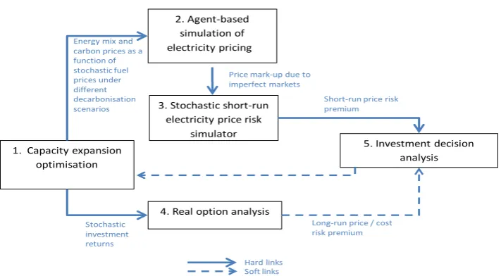
The methodology in this research is developed to adapt the long-term capacity investment scenarios that result from the use of conventional, least-cost optimisation programs with the behavioural implications of imperfect competition (leading possibly to prices above the competitive level) and with some aversion to the risks of financial underperformance (leading possibly to non-investment in NPV positive projects if the downside risks are too high). We therefore seek to develop an integrated and coherent link between these three elements: least-cost planning, strategic behaviour, and risk analysis. Figure 1 displays the overall scheme of module linkages. The hard links between the modules imply that the output files of one module provide the input files for another, in the direction of the link, with all exogenous parameters in common. The soft links suggest that the results of a particular analysis may cause the user to question some of the basic assumptions and re-iterate the analysis.

Figure 1. Schematic of Linkages between Modules

3.1. Module 1: Long-term Least Cost Planning

The analysis begins by developing long-term least-cost expansion plans for the electricity sector, as might be undertaken by a Government to embed various policy targets. In particular, given policy targets for carbon abatement quantities, we include endogenous consideration of carbon price

formation through a carbon market, such as that of the EU ETS. This is distinct from most investment models to support policy and decision-making in the power sector, which assume either exogenous carbon prices, or a relatively simple carbon price formation process (e.g. based on the costs of fuel-switching or the marginal abatement cost of some other particular abatement technology). Similarly, electricity price formation is sometimes approximated by assuming that a particular technology sets the system marginal cost. However, with decarbonisation, we expect deep structural changes to occur in the generation mix which will affect the price formation mechanisms for both carbon and

electricity. In other words, carbon and electricity price are at the same time drivers of, and also driven by, the electricity generation mix. Whilst we develop quite a stylised investment model, we contribute

1. Capacity expansion optimisation

2. Agent-based simulation of electricity pricing

4. Real option analysis

5. Investment decision analysis

Energy mix and carbon prices as a function of stochastic fuel prices under different decarbonisation scenarios

Stochastic investment returns

Long-run price / cost risk premium

Short-run price risk premium Price mark-up due to imperfect markets

Hard links Soft links

3. Stochastic short-run electricity price risk

5

a coherent analysis by seeking to develop carbon price trajectories with technology investment choice and timing determined endogenously to the overall exogenous carbon quantity caps, set as policy targets. As with many carbon markets, the carbon trading is intended to extend beyond a single electricity market, and in taking GB as an example, we need to consider carbon prices being set in the EU-ETS. We therefore construct a two-level formulation to understand firstly how prices are set at the wider regional level of carbon trading, and secondly how these then feed into the investment

economics of a particular, more localised, electricity system.

Thus, we assume a set of possible generation technologies i ∈ {CCGT, coal, nuclear, biomass, OCGT, onshore wind, offshore wind, CCS gas, CCS coal, CCS biomass}. Being a stylised model, not all generation technologies are included, nor are they necessary for the general insights sought. In particular, solar power was excluded, but the explicit effects of intermittent renewables in this model were represented by wind. Key operating characteristics for these technologies include capital cost Γi, fixed operating and maintenance costs FOMi, non-energy variable operating costs VOMi, and heat

rate HRi. Capital costs are calculated as annuitized values, taking into account the overnight capex,

the financial lifetime of the plant and a cost of capital discount rate ρcap. These parameters may vary

over time. We consider a 30 year time horizon, with 7 time steps y ∈ {0,5,10,15,20,25,30}. Any plant built in year y is deemed to have the characteristics associated with vintage v. For example capital costs Γi,v for later vintages will be lower than for earlier vintages if that technology is expected

to benefit from (exogenous) learning effects. Fuel inputs are defined for four main fuel type f ∈ {gas, coal, nuclear, biomass}. Each fuel type is assigned a price in each modelling period, which is an exogenously defined variable PFf,y., and has a carbon emission factor EFf per unit of fuel used.

Demand for electricity is modelled as an inverse load duration curve, which specifies the number of

hours for which demand exceeds a certain level. The curve is divided into 11 tranches, t ∈ {1,…11}; Dt is the total demand in each tranche, ht is the number of hours at which demand is at that level. For

each vintage of technology in each year carbon emissions are calculated as: CO2i,v,y = EFf HRi,v,y ∑t ht

Ci,v,y,t. The key decision variables for the optimisation are the capacities of each technology i of each

vintage v deployed in each year y and in each demand tranche t, denoted as Ci,v,,y,t. The total

generation capacity in each tranche has to at least meet demand, ∑ 𝐶_{𝑡 𝑖,𝑣,𝑦,𝑡} ≥ 𝐷_𝑡 . Since the availability of generation units are below 100%, the installed capacity is higher than expected peak demand creating an effective reserve margin in the model. This margin is about 5% but, as this long-term least cost module is delong-terministic and nonstrategic, neither scarcity prices nor outages appear at this stage, and the main carbon price and generation mix outputs from this module are invariant to the operational reserve. This is in keeping with conventional modelling, whereby the reserve margin is often an exogenous consideration to least cost capacity expansion plans. The reserve margin sensitivity is, however, introduced into the linked risk and strategic modules as described below, where it has a substantial effect.

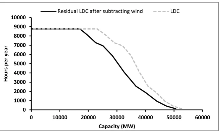
Wind power is intermittent, so the deterministic optimisation cannot dispatch the level of deployment in each tranche separately. Instead, we calculate, for any particular level of wind deployment, the ‘residual load curve’. This is a widely used method and recent examples include Schill (2014), Lise (2013), and Steffen (2013). We therefore subtract, from each demand tranche, the expected

contribution of wind to that particular tranche. Statistically, wind is less likely to contribute to peak tranches than baseload or shoulder tranches and, in this model, it is assumed that expected

contribution of wind to baseload is 33%, whilst its contribution during peak periods is 5%.

6

the resulting impact of wind on the load duration curve is shown in Figure 2 for one particular realisation of the amount of wind in the system:

Figure 2. Example impact of wind on the load duration curve

Carbon capture and storage is modelled as a retrofit technology that can be applied to gas, coal or biomass baseload plants. Capital costs are the marginal costs of the additional plant, marginal emissions are assumed to be negative (so that the combined base plant + CCS have a reduced total emission compared to the base plant on its own).

To model the regional EU-ETS cap-and-trade scheme, the total carbon emissions from the system as a whole, CO2y in year y = ∑ 𝐶𝐶_𝑖,𝑣 2_{𝑖,𝑣,𝑦} , is constrained to meet a cap, CAPy, the level of which is

assumed to be an exogenous variable, set by policy. The price of carbon, PCy , in this case is an

output from this module, and is calculated as the dual variable for the carbon constraint. Banking of allowances between periods is enabled by allowing the model to choose emissions CO2y < CAPy, so

that the difference is carried forward. This raises the cap, CAPy+1 , in the following year. The

optimisation will choose to do this if abatement costs are higher in future years. Borrowing from future allowances is not allowed. At the EU level, the contribution of the other non-electricity sectors within the EU-ETS to meeting the target is based on a simple cost curve approach, taken from EU PRIMES model, and optimised to reduce the degree of emissions reductions required from the electricity sector without affecting the balance of the electricity supply and demand.

The total LRMC of electricity generated by a particular technology i is therefore

LRMC𝑖,𝑣,𝑦= � 𝐶𝑖,𝑣,𝑦,𝑡 𝑡

(𝛤𝑖,𝑣+𝐹𝐶𝐹𝑖,𝑣+ ℎ𝑡𝑆𝑆𝐹𝐶𝑖,𝑣,𝑦)

where the SRMC, in the case of the EU-ETS, is the energy and other variable costs given by:

SRMC𝑖,𝑣,𝑦 = VOM𝑖,𝑣,𝑦+ HR𝑖,𝑣,𝑦𝑃𝐹𝑓,𝑦

Carbon prices calculated from the EU-level model are then passed through to the more detailed local GB market model. The structure of the electricity investment optimisation is the same in principle,

0 1000 2000 3000 4000 5000 6000 7000 8000 9000 10000

0 10000 20000 30000 40000 50000 60000

Ho

urs

p

er y

ea

r

Capacity (MW)

7

except that the carbon price now feeds directly into the calculation of the plant operating costs. Thus, for the GB investment model

SRMC𝑖,𝑣,𝑦 = VOM𝑖,𝑣,𝑦+ HR𝑖,𝑣,𝑦𝑃𝐹𝑓,𝑦+ HR𝑖,𝑣,𝑦𝐸𝐹𝑓𝑃𝐶𝑦

The total system cost for a given year is simply the sum of all LRMC for all plant in the system, plus the cost of offsets and the optimisation objective is to minimise the discounted (at rate ρsys) sum of

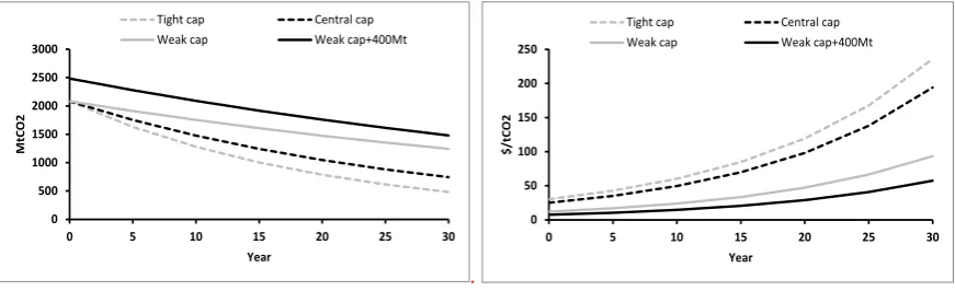
these over the entire 30 year horizon. The parameter estimates and sources are detailed in Appendix 1. With 2012 as the base year, the evolution of the power generation mix is considered under four carbon cap scenarios, as shown in Table 1. These carbon caps are the key exogenous input drivers, and the corresponding carbon price outputs from this module are shown in Figure 3.

Table 1: Exogenous Carbon Abatement Policies

Scenario Annual reduction in cap

Tight cap 5.00%

Central cap 3.50%

Weak cap 1.74%

Weak cap + 400 MtCO2 excess credits 1.74%

Figure 3: Carbon abatement scenarios at the EU level and resulting carbon price outputs

.

(A) Model inputs: EU emissions cap MtCO2 (B) Model outputs: carbon prices ($/tCO2)

The ‘weak’ cap scenario has an annual reduction of 1.74% which corresponds to the rate of reduction specified in the EU-ETS Directive 2009/29/EC, although we apply it as a proportional decline rather than a linear trend. The ‘central’ cap scenario annual reduction is approximately doubled to 3.5% which would be roughly in line with the EU’s more ambitious target of 30% reduction in GHG emissions by 2020, and continuing at this rate thereafter. The ‘tight’ cap scenario considers a faster rate of 5% approximately in line with scenarios that have been suggested for example by the UK’s Climate Change Committee 4th Carbon Budget (CCC 2010).

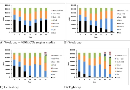
This module does not include any subsidies to support or preclude particular technologies (they are considered in later modules) but wind is forced into the system as a required fraction of generation, to represent the policy requirements under the EU’s targets for renewable energy in 2020. After 2020, the model only introduces wind if it is cost-effective without subsidies. This means that offshore wind starts to retire (whilst onshore wind remains cost-effective and stays in the system). This explains the reduction in wind capacity under the weaker cap scenarios, as displayed in Figure 4. Offshore wind only recovers its share of the generation mix in later years when the carbon price rises under the central and tight carbon caps.

0 500 1000 1500 2000 2500 3000

0 5 10 15 20 25 30

M

tC

O

2

Year

Tight cap Central cap

Weak cap Weak cap+400Mt

0 50 100 150 200 250

0 5 10 15 20 25 30

$/

tC

O

2

Year

Tight cap Central cap

8

Figure 4 Evolution of UK generation mix under four deepening carbon cap scenarios

A) Weak cap + 400MtCO2 surplus credits B) Weak cap

C) Central cap D) Tight cap

Being long term, optimal least cost plans, such results can only really be considered indicative in a centrally planned context, but nevertheless they are often the starting point for long-term policy and fundamental analysis. They leave open the questions of market price formation and the need for investors to earn an adequate return before committing to new capacity. How these mark-ups could be achieved, whether through normal market pricing mechanisms or through additional subsidies, is taken into next the linked modules in the modelling framework.

However, some observations can be made from the outputs of this initial module. Since all of the low-carbon technologies benefit from low-carbon prices increasing steadily over the lifetime of the facilities, annuitized capital costs are only covered in later years. This has two implications. Firstly, with uncertainties in costs and revenues, as well as risk aversion, the benefits of delaying even NPV positive investments may be attractive. Furthermore, if the trajectory of carbon prices changes to become more convex, flatter in early years and steeper towards the end, induced perhaps by market participants making inefficient temporal arbitrage assumptions on the value of banking allowances, this would also increase the value of delay. A later section uses the optimisation model in stochastic mode to identify this potential value of delay using a real options approach.

3.2. Module 2: Strategic Pricing Behaviour

The optimal least cost modelling, as described above, provides a perspective on capacity investment for the EU and GB, taking account of endogenous carbon price formation under an EU-wide target, assuming competitive behaviour. This is the conventional way in which long term baseline pathways are developed. But the analysis does not address what the market prices would have to be for the investments to be attractive to market participants. In the absence of further subsidies, beyond the carbon price, mark-ups above SRMC may be required to achieve the required investment returns,and

0 50000 100000 150000 200000 250000 300000 350000

0 5 10 15 20 25 30

GW

h

Year

Biomass + CCS Gas + CCS Coal + CCS Wind Biomass Nuclear Gas Coal 0 50000 100000 150000 200000 250000 300000 350000

0 5 10 15 20 25 30

GW

h

Year

Biomass + CCS Gas + CCS Coal + CCS Wind Biomass Nuclear Gas Coal 0 50000 100000 150000 200000 250000 300000 350000

0 5 10 15 20 25 30

GW

h

Year

Biomass + CCS Gas + CCS Coal + CCS Wind Biomass Nuclear Gas Coal 0 50000 100000 150000 200000 250000 300000 350000

0 5 10 15 20 25 30

GW

h

Year

9

the question of whether a liberalised market could achieve these is crucial. If generators in a moderately concentrated market can achieve the required mark-ups, it suggests that relaxations of regulatory policy, as an alternative, or supplement, to market subsidies, may become part of the decarbonisation initiatives. This is not such a radical consideration, as SRMC will inevitably diverge from LRMC, as the market share of low marginal cost, high capital cost, renewable technologies increases.

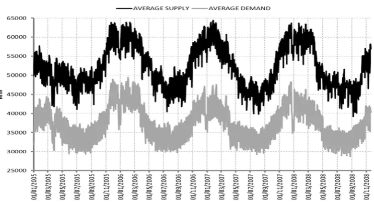
Figure 5 Companies manage availability in response to demand.

In order to set the context for considering market power in this context, we look at real historical behaviour in the GB market as a guide. Even with a relatively unconcentrated market during 2005 to 2008 (average HHI below 1000), the ability of the generators to manage capacity is most remarkably evident in the seasonal pattern shown in Figure , which shows daily average demand and supply over these 4 years. Evidently supply availability was well managed by the generators to maintain a constant capacity margin (the system operator contracts additionally for short term reserve margins), and thereby manage stable prices within and throughout those years (average summer and winter prices were similar despite the annual demand cycle). Further analysis reveals that this intra-yearly capacity management was mainly being carried out by the mid-merit coal plant. With decarbonisation seeking to replace all of this coal, it is evident that a greater intra-yearly role for seasonal capacity profiling will fall upon gas, followed ultimately by nuclear and renewables. Although the generation sector is well-used to coping with low utilisation factors, it is clearly much more tolerable for the larger players. Large players with strong balance sheets and portfolios of assets can temporarily or permanently withdraw capacity without creating the financial distress that a smaller IPP might face.

Thus, the management of capacities and the potential for pricing above marginal cost are

10

Furthermore, there is some empirical evidence on daily behaviour that market participants do not appear to achieve the high prices that theory would prescribe (Wolfram, 1999). This is partly because theoretical solutions to power price gaming usually require highly stylized settings, but more

importantly, the analyses are usually based upon single stage gaming, i.e. one-shot daily or hourly profit maximisation, rather than the repeated game that an oligopoly of generators may seek to maintain over the long term. It is also the case that several researchers have noted that co-ordination in practice is difficult and that real market participants are likely to sub-optimise (Crawford, 2007; Bunn and Day, 2009). Thus, the normative implications of prices from theoretical models of imperfect competition should be treated with caution and almost certainly diluted. Moreover, when market power is exerted in practice it often appears to follow price leadership so that focal points emerge, which may not reflect the fundamental equilibria, but rather manifest local co-ordination around mutually satisfactory outcomes. Thus, econometric models of daily prices tend to show a mixture of fundamental variables such as demand, reserve margin and fuel prices together with lagged variables going back only one day (Karakatsani et al., 2008). More dramatic focal points driven by price leadership occasionally become manifest in apparently classic collusive ways, e.g. Wolak (2000) refers to the punishment strategy invoked by the market-leader, Statkraft, in Norway to sustain a high price level. All of which raises a difficult question on how and to what extent strategic behaviour and imperfect competition should be modelled and evaluated in prospective investment analyses. It would appear realistic to recognise the potential of market participants to achieve prices above the

competitive levels, regulatory surveillance permitting, as this has been large part of the history of liberalised power markets around the world since 1990. Model-based analysis can illuminate this, but given the evidence, gaming models should be more reflective of the bounded rationality seen in practice and at best they should only be considered indicative of what may be possible.

With this perspective in mind, computational learning is increasingly finding application as the most effective methodology to develop insights into price formation in complex markets, where there may be imperfect competition and where analytical results are elusive in all but the over-simplified stylisations. As such, electricity markets have been quite extensively analysed in this way, with a variety of learning algorithms (see Weidlich et al, 2008 for a review). In this research, we have followed a simple and transparent reinforcement algorithm first implemented by Bower et al (2001) to investigate the reform of the British power pool to bilateral trading in 2001. The stylized model is based upon the stack of plant capacities and their marginal costs, together with the 2012 demand distribution consistent with the specification of the optimisation and risk simulation models in the previous sections. In addition, an ownership specification is included, which we choose to specify in various stylized allocations of plant to generic owners, in order not to imply specific behaviour for any currently identifiable companies operating in the GB market. Market clearing is modelled the same way as in the risk simulations. The learning process is iterative based upon repeated offers to the same daily profile. The average daily profile for 2012 is presented repeatedly and the companies may thereby learn, through trial and error, to make offers above SRMC. The agents’ offering strategy is driven by a primary objective of reaching a minimum specified utilisation rate of their plant portfolio and a secondary objective of maintaining or increasing profit once the primary objective has been achieved. By following these objectives through a computational learning algorithm, the agents learn the profit-maximising policy, subject to utilisation, for offering capacity and prices for all their plants in the daily auction.

11

Each agent has a minimum utilisation hurdle𝑈_𝑖 which it wants to exceed.

Each unit j of agent i defines its offer price,𝑃_𝑖𝑖 , as marginal cost, 𝐹𝐶_𝑖𝑖, plus mark-up, 𝐹𝑈_𝑖𝑖. For all ij at learning iteration k, we have 𝐹𝑈_𝑖𝑖𝑖 and Profit Contribution 𝑃𝐶_𝑖𝑖𝑖

For all ij at learning iteration k, we record the previous change in offer prices at each plant

𝐷𝑃𝑖𝑖𝑖

For all agents we have total market portfolio Profits 𝑃𝐶_𝑖𝑖, and Utilisation 𝑈_𝑖𝑖. At iteration k,

If 𝑈_𝑖𝑖−1>𝑈_𝑖, go to B; if not go to A;

A: Reduce 𝐹𝑈_𝑖𝑖𝑖 of all units individually by separate random e1 values subject to merit order

conditions.

B: if 𝑃𝐶_𝑖𝑖 >𝑃𝐶_𝑖𝑖−1 , repeat 𝐷𝑃_𝑖𝑖𝑖, if not, revert to the previous offer at 𝐹𝑈_{𝑖𝑖𝑖−1}, in each case with the addition of a small random value, e2.

[e1 is positive with a range (0,E1), e2 varies about zero with a range (-E2, E2)] Repeat to iteration 𝑘+ 1

Record average market price (𝐴𝐴𝐹𝑃_𝑖) for final half of the iterations.

Merit order needs to be preserved, so random adjustments are constrained never to lead to offers that would reverse the basic marginal cost merit order of the units within each agent’s portfolio. This means that at any iteration, for all units in company j, offer prices, 𝑃_𝑖𝑖𝑖, should be nondecreasing in i. While the desired rate of utilisation is defined exogenously, the profit objective is pursued

endogenously: each generator is continuously learning to improve performance in the profit objective using the previous trading day’s profit as a benchmark to evaluate the current day’s performance. There are several reasons why companies will want to maintain a utilisation target. This could be part of their long-term market share strategy, or it could reflect prior contracting, or in some cases it could reflect availability obligations promised to the regulator. As will be seen later, assumptions about utilisation are critical to price formation, but if a low utilisation hurdle is selected, then it provides a basis for the company to substantially withdraw capacity, or indeed, if sustained, shrink in size.

It should be re-emphasised that the outputs of such a strategic model should only be considered indicative of what might be possible. How real agents will chose to co-ordinate is highly speculative; sometimes less so than models of imperfect competition would suggest, sometimes more collusively. Furthermore, even in the simple setting of a symmetric duopoly, without demand elasticity, where offers are for a fixed amount of capacity, the often-cited work by Fabra et al (2006) informs us that there will be three equilibrium solution regions, one at the competitive level for low demand, one unbounded or at a cap for high demand and an intermediate region of indeterminate or mixed strategies. The intuition is that in the intermediate conditions, the incentive to undercut when one agent is moving the prices up creates the potential for cycling behaviour. In our more complex setting, the solution regions are not amenable such simple analysis, but we expect a similar perspective that pure equilibria may often not exist. As such, computational learning models can at best only be indicative of the potential for co-ordination.

For the purposes of this analysis, the basic moderately concentrated scenario is a stylization of the GB market in 2012 with six large generators (“Big 6”) and a competitive fringe, which is assumed to comprise the excess capacity in the system, and which does not behave strategically. We assume the Big 6 are symmetric in terms of size and technology ownership. We then go on to consider

consolidations of the Big 6 to produce Big 5, Big 4, Big 3 and Big 2 market structures in a similar symmetric way. Later we relax the symmetries.

12

year which averages 39.5GW, with a maximum 54GW6. With this amount of excess capacity, if the competitive fringe seeks to be fully utilised, then the strategic players will be forced to withdraw substantial capacity in order to support prices, as they have done in GB since 2012, and as a consequence operate within our model at low average utilisation levels around 50%.

Without excess capacity and a competitive fringe, strategic behaviour by a symmetric group of six or less generators would always lead to unbounded prices. For simplicity in the initial experiments, we assume that decarbonisation takes place through the activities of the big players, and that the competitive fringe stays constant. The competitive fringe consists of 50 facilities (denoted by

“Others” in the figures below). We have two variations of reserve margin/competitive fringe; one with 34% of the market and another with 15%. The types of technologies associated with the competitive fringe are offshore wind, onshore wind, OCGT, CCGT, and biomass, distributed across 20 owners. We start with exactly 77815 MW installed and initially take the case of 15% in to the competitive fringe. Average demand is about 40GW. So if the fringe always dispatches at 90%, ie almost 12GW, it leaves about 28GW on average of demand to be covered by the strategic players who own 64252 MW. Thus, if the strategic players’ utilization targets are close to 50%, on average they will be competing with the competitive fringe and prices will be close to marginal cost. If they are willing to come down to 40% or below on average, then one of the players could become pivotal and prices may be unbounded. In theory, therefore, if they are all able to move capacity utilization down to the required level, very high prices can be maintained and all investment could be supported.

Alternatively, if they all seek too high a level of utilization, prices will be driven to competitive levels. In between these extremes, co-ordinating and maintaining prices may be delicate as one player may be unwilling to take on the role of the residual price maker, even if it leads to higher profits, as that may involve accepting substantially lower utilization than the other symmetric large players.

Furthermore, in practice with demand and supply fluctuating hourly, the convergence of offers will be even harder to learn than in this experimental setting where the same daily demand profile is

repeatedly presented to the computational agents.

In this study, we are seeking therefore to understand plausible multi-agent behavior in moving and maintaining offers above marginal cost to exercise market power, and so the initial trajectories of learning over 100-200 iterations are most revealing in terms of identifying the relative ease of co-ordination, given that with very extensive learning on the same market situation, unbounded prices will always be possible in our experiments. We accept the evidence that market participants tend to adjust their offers in a cautious adaptive manner with bounded rationality, and we advanced the simple reinforcement learning algorithm with that in mind. Recall that the reinforcement behavior is simply one of repeating or reversing previous offers, plus a small random search, to maintain or improve profits subject to minimum utilization. Furthermore, in pursuing it, it is likely that the search for improved performance by market participants will be gradual. These conjectures are important, as tuning the search parameter in the algorithm is quite delicate, as indeed is setting a plausible lower bound for utilization levels7. The following indications from running this module as a standalone function set this context.

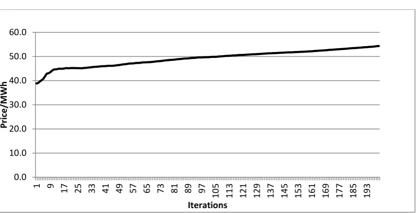
If we allow substantial withdrawal by any of the strategic players, down to as low as 30%, and look at the initial state, with the six strategic players seeking to co-ordinate, Figure 6 shows that the agents steadily learn to increase prices, as indeed theory would suggest.

6

Demand was low in 2012 because of the post 2008 recession. Highest recorded GB demand was 60.1GW in December 2002

13

Figure 6. Agents learn to increase prices

Most revealing is to study how they do this by looking at their utilisations. We found that after a period of large swings in utilisation, the market settles with two companies accepting the lower utilisation (around 35%) role of being the price makers, and the others having the higher load factors, closer to their maximum (80-90%, taking annual planned and unplanned availabilities into account). With symmetry, evidently the particular companies found and locked into such relative roles randomly. Once a company has settled into the role of being the marginal price-setter, then prices increase steadily. It does not follow however, that the more concentrated the market becomes, the easier it is to co-ordinate and increase prices more steeply. Recall the earlier reference to the symmetric duopoly theory (Fabra et al 2006), which suggests that if the agents are offering a fixed capacity, then there are three solution regions, marginal cost for low demand, unbounded at high demand and mixed strategies in between. In our setting, if we were to merge the six companies into two, we would be in a low demand setting if they tried to sell all (80-90%) of their capacity. Low prices would emerge from the repeated attractions of undercutting whenever one player raised prices. We found in this case that prices became locked into a cycle, as the company that has taken on the lower utilisation seeks repeatedly to undercut and increase market share. A similar process emerges if we have an asymmetric triopoly. The larger companies, as theory suggests, take the lower utilization roles, but even here, we see slow escalation of prices. We see a quicker price rise if we set a minimum 30% utilization target from the outset.

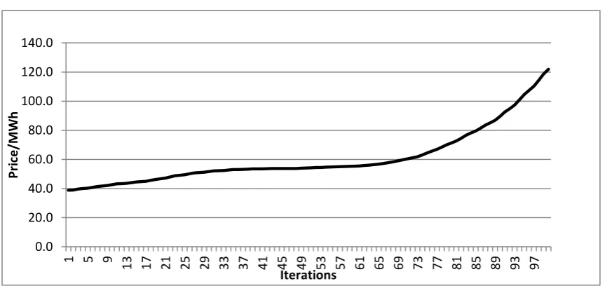
An important variant of this investigation was to explore asymmetry in the distribution of plant technologies across owners according to the allocations Table 2. In this Table, the six companies are labelled AAA, BBB, etc. We see slightly lower prices and a more difficult co-ordination process than in the symmetric in the Big 6 case. However, if we allow AAA to merge with BBB and CCC thereby concentrating all CCGT and Coal power plants into a single company, this focusses market power and leads to a more dramatic prices, as in Figure 7. Now, only in very few cases do utilization rates fall below 30% and, as a result, average daily prices reach £120/MWh within 100 iterations and seem set to escalate thereafter even more quickly. Thus, it is clear that mergers allied to technology niches is clearly a crucial aspect of achieving market power results more easily in a moderately concentrated market.

0.0 10.0 20.0 30.0 40.0 50.0 60.0

1 9 _{17 25 33 41 49 57 65 73 81 89 97}

10

5

11

3

12

1

12

9

13

7

14

5

15

3

16

1

16

9

17

7

18

5

19

3

Pr

ic

e/

M

W

h

14

Table 2. Share of each plant type amongst the big 6 companies

Figure 7. Pricing behaviour when CCGT and coal plant are owned by a single company

3.3. Module 3: Short-run Market Price Risk

The third key element we need to introduce into considerations of investability in the power sector is the short-run (intra-year) price risk. We take the view that investors will acknowledge long-term least- cost modelling for providing a view of where market fundamentals are driving the industry, the way in which policy makers will think about interventions, and therefore how the long-run structure of the industry is likely to evolve in terms of generation mix. Investors may, however, be quite cautious about the sustainability of market power. Typically, when it comes to the final investment decision point for an individual project, lenders and investment committees examine a detailed financial model that makes explicit analysis of risk, and in particular, if it is viewed as a project, the risk that the annual net operational earnings will cover the financing costs (i.e. the “coverage ratio”, as in CPI, 2011; Moody’s, 2009).

In order to focus precisely upon the annual financial performance risks of assets, therefore, particularly with respect to coverage ratios under progressive decarbonisation, the risk analyses developed here are formulated as a series of detailed, specific year analyses of the output from the optimisation and strategic modules. This allows for a probabilistic simulation of operational and price

0.0 20.0 40.0 60.0 80.0 100.0 120.0 140.0

1 5 9 _{13 17 21 25 29 33 37 41 45 49 53 57 61 65 69 73 77 81 85 89 93 97}

Pr

ic

e/

M

W

h

15

risks within a particular year, based upon empirical data, so that annual operational profit probability distributions can be compared with annuitized financing costs. The long-term specifications result from least cost optimisation module. Essentially these longer term parameters set the mean values for each year, which may have price mark-ups determined by the strategic simulations, and the target year risk simulations analysed here are calibrated to intra-year variations around such means. The annual risk model is much more detailed in its modelling of stochastic supply and demand effects than in the longer term investment scenarios of module1.

Wind speed is now represented in this module using Weibull probability distribution functions, and this is converted to power according to a typical wind-power nonlinear transfer function, following Zonneveld et al (2008), Kusiak (2008) and Hossain et al (2011), leading to an average annual production of around 30% of installed capacity. The portfolio averaging of extensive wind farm penetration is modelled by considering two regions in GB, north and south. From studies on wind speeds in geographic locations (Sinden, 2007) an output correlation index of 0.7 is taken for plants in the same geographic areas within the north or south, and an index of 0.1 is used between the north and south plants. New offshore wind generation is assumed to be distributed evenly between north and south. The model is formulated as a ‘stylised’ scenario-based model in which market structure follows the outputs of the long-term optimisation model and the agent behaviour may be competitive (at marginal cost) or strategic with mark-ups determined by the computational learning of module 2.

In the stylised GB model no allowances were made for start-up costs, but the market price

uncertainties in EU carbon allowances are included, having been estimated empirically around yearly means over previous years. Transmission constraints do not factor into wholesale market prices, as they are part of the real-time system balancing activities. We have negative marginal costs for wind implied by the renewable subsidies (ROCs). This means that these generators would, if necessary, be willing to pay up to the value of their subsidy in order to produce; hence the negative wholesale prices that sometimes appear (especially in Germany and Denmark where wind penetration was much higher than GB in 2011). Parametric values are sampled statistically as Monte Carlo simulations. A winter and summer demand are sampled repeatedly to form seasonal hourly demand distributions, based upon the actual 2012 hourly data. This seasonal split is designed to interact with typical seasonal availabilities for the generating facilities. No demand elasticity is assumed. Unplanned outages are simulated according to binomial distributions based upon average availabilities.

Fossil-fuel prices are sampled from log-normal distributions with intra-yearly standard deviations and correlations estimated empirically over recent years as follows:

Correlations Oil Gas Coal

Oil 1

Gas 0.631 1

Coal 0.861 0.628 1

The module simulates hourly market prices and utilisations for each plant, thereby returning statistical distribution for annual profit contribution for each plant in the system. These can also be aggregated by company ownership. New investment performance is monitored in terms of annual profit

16

ratio above 1 means that the asset is making a positive return, and that would be comparable to an NPV criterion. Following the risk simulation analysis, we have a probability distribution for this ratio and a critical value exceeding 1.2 with 95% confidence is taken as an indicative criterion that may be considered by analysts and ratings agencies to retain an investment grade (CPI, 2011). Although, as a baseline, 100% debt financing of new assets was assumed, it is recognised that typically, onshore wind assets have been 80% debt financed in GB, offshore rather less, and CCGT/coal/nuclear generally being on-balance sheet. However, for some rather fundamental comparative insights, these baseline assumptions were taken to provide a reasonable and conservative proxy for the range of financial performance metrics that may be used in practice (since for leverage below 100%, higher equity returns than debt will generally be required). For this reason we refer to this ratio more generally as capital coverage in what follows. In any particular case, a company’s idiosyncratic tax, leverage, amortisation and corporate circumstances will, of course, be quite distinctive.

4. Integrated Results

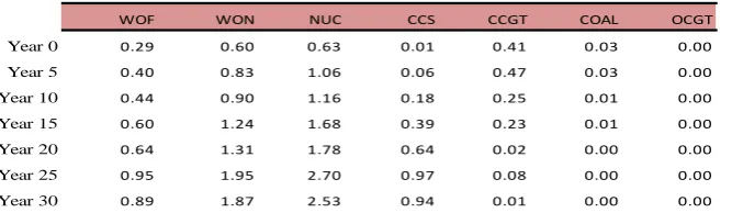
We report first the output from the stylised version of the investment risk simulation module 3, linked to the output from module 1 but without the strategic behaviour being activated through module 2. This is therefore a competitive market baseline. Risks are simulated, as above, for each of the 5-year modelling periods according to the outputs from the long-term optimisation model. Table 3 shows the 5th percentile values for the distribution of capital coverage ratios for each of the main technology types covered in the model8. The scenario represented here is the central carbon cap, and assumes a high nuclear cost scenario. No further subsidies are assumed for low-carbon plant in this scenario. In order to meet the capital coverage threshold, the 5th percentile should be above 1.2. In the early years until year 15, for this scenario, the results of risk simulation indicate that none of the technologies would meet the criterion of debt coverage exceeding 1.2 with 95% probability. By year 15, and thereafter, with the higher carbon prices coming through, nuclear and onshore wind meet the criterion, but that is all. In fact, similar results have been produced, but not reported here, for all the other carbon cap scenarios that do not include any low carbon subsidies.

Table 3. 5th Percentile value of capital coverage ratios

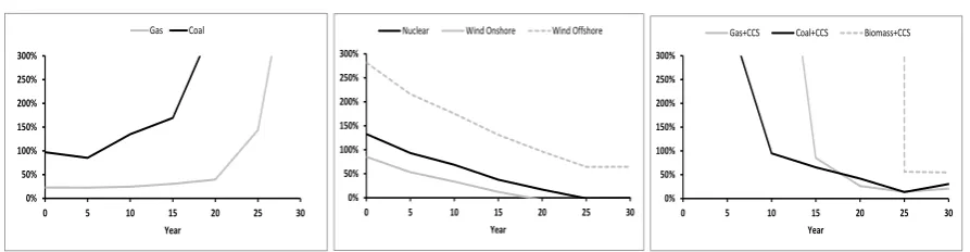
In other words, the risk neutral view of least cost planning in the aggregate would be confronted by risk-averse financial planning considerations at the level of the firm. The consequences of this are various. There could be a capacity-building hiatus, until scarcity induced higher prices, or it is possible that prices could be raised by firms with sufficient market power, or there could be further subsidies. We will revert to a discussion of these remedies later. Figure 8 shows the significant level of mark-up above system short-run marginal cost that would be required in order to raise up these

8

WOF: wind offshore, WON: wind onshore, NUC: nuclear, CCS: coal with carbon capture and storage, CCGT: combined-cycle gas turbine, COAL: coal, OCGT: open-combined-cycle gas turbine.

WOF WON NUC CCS CCGT COAL OCGT

Year 0 0.29 0.60 0.63 0.01 0.41 0.03 0.00

Year 5 0.40 0.83 1.06 0.06 0.47 0.03 0.00

Year 10 0.44 0.90 1.16 0.18 0.25 0.01 0.00

Year 15 0.60 1.24 1.68 0.39 0.23 0.01 0.00

Year 20 0.64 1.31 1.78 0.64 0.02 0.00 0.00

Year 25 0.95 1.95 2.70 0.97 0.08 0.00 0.00

17

coverage ratios so that they exceed a factor of 1.2 with 95% probability. Evidently, to be able to up revenue in this way requires that the whole supply function is lifted uniformly by the mark-up, which, in the absence of subsidies, requires co-ordination amongst all owners of all technologies.

Figure 8. Price mark-up above system marginal cost required to reach 95% probability of capital coverage ratio >1.2 for various technologies under the central carbon cap scenario.

The short-run risks for gas and coal plant increase quite substantially in the intermediate years. Under the central scenario, the coal plant becomes steadily less attractive anyway because of rising carbon prices. For gas plant, the risk arises due to the potential future addition of newer gas plant to the system with an expected improvement in efficiency which would push the current vintage gas plant further down the merit order and increases the risk that it may not get deployed. This indicates that investors in fossil-fired plant either need to plan on recouping their investment in the initial 10 to 15 year period, or perhaps consider other ways of assessing their willingness to accept short-run risk.

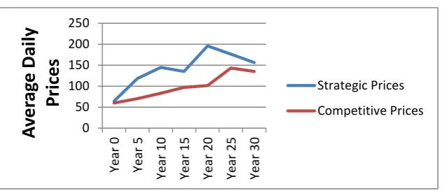
It was evident from the initial simulations of the strategic module, in section 3.2 above, that mark-ups in this stylised setting can be substantial and will depend upon the reserve margin, the degree of concentration and the diversity of technology ownership. All of these dimensions of market structure can be expected to be co-evolutionary, if allowed, as the industry re-organises itself to meet the required profits. The insights from the strategic simulations in section 3.2 suggest that even the moderately high mark-ups required in Figure 8 for the low carbon technologies over the medium and longer terms are within reach for a concentrated industry. Additional complexity in the market power effects also comes from its uneven dynamic properties. For example, if we compare the relatively unconcentrated and over-supplied market structure of the basic six symmetric companies and a 34% competitive fringe, acting strategically and competitively, and evolving over time in response to the changes in generation mix consistent with the outputs of the long-run optimisation module 1, with the central carbon-cap, high nuclear-cost reference scenario, we see an uneven emergence of market in Figure 9.

Figure 9. Electricity price evolution with 34% competitive fringe

0% 50% 100% 150% 200% 250% 300%

0 5 10 15 20 25 30 Year

Gas Coal

0% 50% 100% 150% 200% 250% 300%

0 5 10 15 20 25 30 Year

Nuclear Wind Onshore Wind Offshore

0% 50% 100% 150% 200% 250% 300%

0 5 10 15 20 25 30 Year

Gas+CCS Coal+CCS Biomass+CCS

0 50 100 150 200 250 300

Year

0 Year5 Year10 Year15 Year20 Year25 Year30

Av

er

ag

e Daily

Pr

ic

es

18

The strategic prices are those which emerged after 100 learning iterations. Evidently these are not equilibrium prices but for the reasons mentioned previously, we feel it is more constructive to look at the relative speed of learning to consolidate, as a way of differentiating the strategic potential in the various scenarios. As for the Year 0 analysis reported in 3.2, we again look at the sensitivity to different scenarios for the size of the reserve margin and competitive fringe of 15% and 34%. In both cases, the ability for companies to manage prices upwards is very evident, but with 15%, the pattern was similar, but with higher prices. The evolution of market power is evidently, therefore, non-monotonic over time. Market power increases to a local peak after ten years, as the Big 6 retain price–setting with gas plant, and are able to increase inframarginal profits though the replacement of some of coal facilities with the lower marginal cost wind eroding prices. They are therefore able to operate their fossil price-setting plant more aggressively. With further decarbonisation, however, they lose this price-setting benefit, the competitive fringe is more influential, and mark-ups decline. Finally, after 30 years, market power returns as some CCS facilities, together with high gas and carbon prices increase the price setting capabilities at the margin. The subtle interaction of the profile of technological change and market concentration is therefore revealed. Furthermore, policy affects this non-monotonicity as well. With a tighter carbon cap, prices are higher in earlier years as shown in Figure 10, with a remarkable change in the profile of market power evolution. It seems that the increased pace of decarbonisation opens up the market power potential sooner.

Figure 10. Electricity price evolution with a tight carbon cap

Overall, as these mark-ups are substantial and compare to the risk premia identified previously, these results suggest that once the companies have determined their lowest mutually acceptable utilization levels, co-ordination to increase prices is possible, leading to adequate investment support, even with six similar companies operating. This will presumably be easier the less excess capacity is in the system, and the process of withdrawing excess capacity is easier, the more concentrated the market. Thus, market consolidation may be a precursor to effective strategic pricing support for decarbonizing investment, in the absence of substantial subsidies. Furthermore, consolidation and technology specialization may offer greater potential for price movers, which may imply that market power will emerge unevenly as decarbonisation trajectories evolve.

As a consequence of these insights, the ability to achieve adequate investment returns in an energy only market through strategic behaviour is evidently idiosyncratic to the specific market under

consideration, its level of concentration, capacity mix, reserve and the ability of market participants to learn collusive outcomes. To give a final focus to this we therefore look at a more specific example, with the GB market under its ownership structure in 2012 (ie not stylized into the AAA, BBB, etc, companies as above) and consider how investability in this market in 2012 would vary if wind progressively replaced more of the 26GW of coal in the system at that time. This is not a forward

0 50 100 150 200 250

Yea

r 0

Yea

r 5

Yea

r 1

0

Yea

r 1

5

Yea

r 2

0

Yea

r 2

5

Yea

r 3

0

Av

er

ag

e Daily

Pr

ic

es

19

looking scenario, but a sensitivity analysis of 2012, with all of the 2012 parameters, if it had different replacement levels of coal by wind. The coverage ratios that would result for wind, nuclear and gas, under competitive offers and with strategic learning (100 iterations) are shown in Figure

Table 4: Investment Coverage Ratios in the 2012 GB market if wind replaced coal

Each cell gives the average coverage ratio, and we notice that it declines with more decarbonisation. The shaded cells are where the P95 criterion of being greater than 1.2 is not met. Evidently, when 21 of the 26GW of coal are replaced with wind, none of the technologies would meet the coverage ratio criterion without further help, or a tighter reserve margin, or greater market concentration. On the other hand, strategic behaviour would support all investments in the base case, and offshore wind up to 14 GW replacement. The circumflexes in the base case cells indicate that the prices were rising rapidly even before 100 iterations and the investment criterion would have been met comfortably and restrained only by a price cap.

5. Risk and Delay

Finally we consider possibility that in response to not meeting the risk criteria and without the ability to rely upon the exercise of market power (eg for regulatory concerns), investors may choose to delay and create an investment hiatus. Evidently, this will cause prices to rise, depending upon demand growth and plant retirements, but it will also affect the trajectory of carbon prices. We therefore feed this consideration back into module 1 to see what it would do to carbon prices. Figure 11 displays this. Evidently, carbon emissions rise during the period of the investment hiatus because of the greater reliance on existing fossil plant, some of which is old and less efficient. The higher emissions lead to higher carbon prices in the short and medium periods of the modelling horizon. This arises because more carbon allowances are required in the early period to cover the greater use of fossil fuel plant, so fewer allowances are available to bank through to later periods. Furthermore, higher carbon prices in turn would improve the investment case for new plant because they raise the expected electricity price.

GW Coal Replaced

Base Case

7

14

21

Wind Offshore

Competitive

1.3

1.3

1.3

1.2

Wind Offshore

Strategic

^

1.75

1.7

1.3

Nuclear Competitive

0.9

0.8

0.7

0.6

Nuclear Strategic

_^

1.8

1.6

0.8

CCGT Competitive

0.7

0.4

0.3

0

20

Figure 11. Impact of investment hiatus on carbon price trajectory (average of all cap scenarios)

When companies are faced with the choice of making an irreversible investment in a project with uncertain future returns, there can be a real options value in waiting if this allows the company to avoid some downside risk. However, the cost of waiting will eventually outweigh the value of waiting, and rational investors would choose to proceed at that point. To evaluate this real option, we use an approximation to dynamic programming (as in Dixit, 1994), whereby the optimisation model is run N times, with different realisations of the main stochastic variables for each run. The average NPV across all N runs is evaluated for each time period t, and the value of waiting is calculated, assuming that the evolution of the overall market is unaffected by this decision to delay. We evaluate average mark-ups above SRMC in order for investing immediately to be a better opportunity than the option of waiting until Year 5. The mark-ups depend on the stochastic parameters (see Appendix 1) which are mainly based upon the DECC 2050 pathways calculator, DECC (2011) and Parsons Brinkerhoff (2012).

As a result, Figure 12 reports the mark-ups required to bridge different investment hurdles following the feedback effects of delayed investment. The charts show the ‘Breakeven’ mark-ups required to achieve a positive NPV, based on the expected value across all the stochastic scenarios evaluated at 7% discount rate as well as the mark-ups required to bring capital coverage ratio (CCR) above either 1.0 or 1.2 in 95% of outcomes. The CCR>1.0 is shown for sensitivity, and might be appropriate for larger companies able to accommodate short-run risks. The Long-run mark-up (LR) evaluates a premium based upon the dispersion of annual average values over time (as produced by module 1) whereas the LR+SR premium considers both this long run and the short run premia to meet the additional intra years risks, as evaluated through module 3. Evidently, in focussing upon the mark-ups required, we are again suspending the strategic learning in module 2, but we observe that these mark-ups are within reach of the strategic behaviour as evidenced in the previous simulations

On the horizontal time axis, a distinction is made for the case of investing in year 5 or 10 where the market evolves according to the optimal plan and the ‘delay’ case in which no new plant is built by any players in the early periods. In the delay scenarios (5-year or 10-year), the retirement profile for existing fossil-fired power plants is relaxed so that there is sufficient existing plant on the system to meet demand over the full 10 year period until a new plant is built. Compared to no delays, the improvement in expected returns resulting from the investment hiatus is noticeable for the low-carbon generation sources, but it takes ten years to show up. It is important to recognise that in this analysis, it is not due to prices rising because of scarcity; we maintain the same level of security by retaining

0 20 40 60 80 100 120 140 160 180

0 5 10 15 20 25 30

Ca

rb

on

P

ric

e

$/

tC

O

2

Year

21

facilities that otherwise would be retired. Rather it is the endogenous effect of carbon prices rising and thereby reducing the risk premia required to initiate investment. Total emissions are higher in the short term, but lower in the longer term since the optimal investment trajectory is still required to meet the same final cap. Overall, the endogenous nature of carbon and electricity markets appears to be somewhat self-correcting. However, we see that for wind and CCS, even after ten years, with the hiatus-induced higher carbon prices, further financial support, or the market power to achieve prices above SRMC would be required.

Figure 12. Evolution of investment conditions over time and under an investment hiatus

-50% 0% 50% 100% 150% 200%

Yr 0 Yr5 Yr5 delay Yr10 Yr10 delay

M

ark

-u

p

Gas+CCS LR+SR premium CCR>1.2 LR+SR premium CCR>1 LR risk premium Breakeven NPV=0

-50% 0% 50% 100% 150% 200%

Yr 0 Yr5 Yr5 delay Yr10 Yr10 delay

M

ark

-u

p

Coal LR+SR premium CCR>1.2 LR+SR premium CCR>1 LR risk premium Breakeven NPV=0

-50% 0% 50% 100% 150% 200%

Yr 0 Yr5 Yr5 delay Yr10 Yr10 delay

M

ark

-u

p

Coal+CCS LR+SR premium CCR>1.2 LR+SR premium CCR>1 LR risk premium Breakeven NPV=0

-50% 0% 50% 100% 150% 200%

Yr 0 Yr5 Yr5 delay Yr10 Yr10 delay

M

ark

-u

p

Nuclear LR+SR premium CCR>1.2 LR+SR premium CCR>1 LR risk premium Breakeven NPV=0

-50% 0% 50% 100% 150% 200%

Yr 0 Yr5 Yr5 delay Yr10 Yr10 delay

M

ark

-u

p

Biomass+CCS LR risk premium Breakeven NPV=0

-50% 0% 50% 100% 150% 200%

Yr 0 Yr5 Yr5 delay Yr10 Yr10 delay

M

ark

-u

p

Onshore Wind LR+SR premium CCR>1.2 LR+SR premium CCR>1 LR risk premium Breakeven NPV=0

-50% 0% 50% 100% 150% 200%

Yr 0 Yr5 Yr5 delay Yr10 Yr10 delay

M

ark

-u

p

Offshore Wind LR+SR premium CCR>1.2 LR+SR premium CCR>1 LR risk premium Breakeven NPV=0 -50% 0% 50% 100% 150% 200%

Yr 0 Yr5 Yr5 delay Yr10 Yr10 delay Mark

-up