City, University of London Institutional Repository
Citation: Ballotta, L. ORCID: 0000-0002-2059-6281 and Fusai, G. ORCID:
0000-0001-9215-2586 (2018). Tools from Stochastic Analysis for Mathematical Finance: A Gentle Introduction (10.2139/ssrn.3183712). SSRN Working Paper Series.This is the draft version of the paper.
This version of the publication may differ from the final published
version.
Permanent repository link: http://openaccess.city.ac.uk/20049/
Link to published version: http://dx.doi.org/10.2139/ssrn.3183712
Copyright and reuse: City Research Online aims to make research
outputs of City, University of London available to a wider audience.
Copyright and Moral Rights remain with the author(s) and/or copyright
holders. URLs from City Research Online may be freely distributed and
linked to.
Electronic copy available at: https://ssrn.com/abstract=3183712
A Gentle Introduction
Laura Ballotta
1Gianluca Fusai
2May 23, 2018
Electronic copy available at: https://ssrn.com/abstract=3183712
The idea of this document is to provide the reader with an intuitive, yet rigorous and comprehensive introduction to the main tools in stochastic analysis required in Finance to understand the modern modelling, pricing and hedging techniques.
We would like to emphasize that this document is very much work in progress and we would like to encourage readers to get in touch with us with feedback, comments, suggestions for additions and, of course, corrections of typos. All of these will be gratefully acknowledged in the future releases of this document.
Few implemented examples for each model discussed here can be found on the website https://sites.google.com/uniupo.it/stochasticcalculus/home?authuser=1.
If you have suggestions please contact us at the following email: [email protected]
Laura Ballotta and Gianluca Fusai
A Gentle Introduction to Stochastic Calculus in Continuous Time
I
A Gentle Introduction to Stochastic Calculus in Continuous Time
3
1 Aims 7
2 The Brownian motion 9
2.1 Defining the Brownian Motion . . . 10
2.1.1 The odd properties of the Brownian Motion . . . 10
2.1.2 Density of the Brownian Motion at different Time Horizons . . . 11
2.1.3 The (auto)-covariance function . . . 12
2.1.4 Correlated Brownian motions . . . 13
2.1.5 Martingale property . . . 14
2.1.6 Scaling property . . . 15
2.1.7 Markov property . . . 16
2.1.8 Simulation of Brownian sample paths . . . 17
2.1.9 Total Variation . . . 17
2.1.10 Quadratic Variation . . . 19
2.1.11 Properties of the Increments of the BM . . . 23
3 The Stochastic Integral and Stochastic Differential Equations 25
3.1 Introduction . . . 26
3.2 Defining the Stochastic Integral . . . 26
3.3 The Ito stochastic integral as a mean square limit of suitable Riemann-Stieltjes sums . . . 27
3.4 A motivating example: ComputingR0tW(s)dW(s) . . . 28
3.4.1 Example: ComputingR0tW(s)dW(s)by simulation . . . 28
3.5 Properties of the Stochastic Integral . . . 28
3.6 Stochastic integrals as Time Changed Brownian Motions . . . 32
3.7 Ito process and Stochastic Differential Equations . . . 36
3.8 ABM with deterministic volatility . . . 36
3.8.1 Matlab: Simulating the Arithmetic Brownian Motion . . . 39
3.9 Solving Stochastic Integrals and/or Stochastic Differential Equations . . . 42
3.9.1 Deterministic vs. Stochastic Differential Equations . . . 43
3.9.2 Examples of stochastic differential equations . . . 45
3.9.3 Existence and uniqueness of the solution . . . 45
4 Introducing Ito’s formula 47 4.1 A fact from ordinary calculus. . . 48
4.2 It ˆo’s formula whenY =g(X),g(X)∈ C2 . . . 49
4.3 Guiding principle . . . 50
4.4 It ˆo’s formula whenY(t) = g(t,X),g(t,X) ∈ C1,2 . . . 50
4.5 The Lamperti transformation . . . 52
4.5.1 Example . . . 53
4.6 The Multivariate Ito’s lemma whenZ= g(t,X,Y). . . 54
4.6.1 Examples . . . 56
5 Important SDEs 58 5.1 The Geometric Brownian MotionGBM(µ,σ) . . . 60
5.1.2 Solving the SDEdX =µXdt+σXdW . . . 61
5.1.3 Matlab Implementation: Simulating GBM . . . 64
5.1.4 Remark. GBM with deterministic drift and volatility . . . 68
5.2 The Vasicek Mean-Reverting process . . . 75
5.2.1 A Note: The Ordinary Differential Equationdx(t) = α(µ−x(t))dt. . . 76
5.2.2 Solving the SDEdX(t) =α(µ−X(t))dt+σdW(t) . . . 79
5.2.3 The (auto)-covariance function . . . 80
5.2.4 Matlab: Simulation of the Vasicek model . . . 81
5.2.5 Extension: MR with deterministic volatility . . . 87
5.3 The Cox-Ingersoll-Ross (CIR) model . . . 89
5.3.1 Solving the SDEdX(t) =α(µ−X(t))dt+σpX(t)dW(t) . . . 89
5.3.2 Computing the expectation of the CIR model . . . 90
5.3.3 Computing the variance of the CIR model . . . 91
5.3.4 Again on computing the variance and the auto-covariance of the CIR model . . . 92
5.3.5 The distribution of the short rate in the CIR model . . . 94
5.3.6 The Extended-CIR model . . . 97
5.3.7 Simulating the CIR model . . . 100
5.4 The Constant Elasticity of Variance (CEV) model . . . 106
5.5 CIR, CEV and the Bessel Process . . . 116
5.6 The Brownian Bridge . . . 118
5.6.1 A Note: The Ordinary Differential Equationdx(t) = (b−x(t))/(T−t)dt. . . 118
5.6.2 Solving the SDEdXt = (b−X(t))/(T−t)dt+dW(t) . . . 119
5.6.3 Matlab Implementation: Simulating Brownian motions (part 2) . . . 121
5.7 The Heston Stochastic Volatility model . . . 126
5.7.1 The characteristic function of the log-price . . . 128
5.7.2 Heston model: Monte Carlo Simulation . . . 134
5.7.3 Recovering the density function in the Heston model via inversion of the characteristic function . . . 138
5.7.4 Heston model and option pricing . . . 144
5.8 The Heston app . . . 152
6 Stochastic Processes with Jumps 155 6.1 Preliminaries . . . 156
6.1.1 The Poisson process . . . 156
6.1.2 The Compound Poisson process . . . 158
6.1.3 The Gamma process . . . 159
6.1.4 Simulation of Jump Processes . . . 160
6.2 Jump Diffusion (JD) processes . . . 163
6.2.1 The Merton Jump Diffusion Process . . . 163
6.2.2 The Kou process . . . 173
6.3 Subordinated Brownian motions . . . 176
6.3.1 The Variance (VG) Gamma process . . . 177
6.4 Final Remark: L´evy processes . . . 184
6.5 Jumps versus Stochastic Volatility . . . 185
7 Changes of Measure 191 7.1 Preliminaries . . . 192
7.2 Girsanov Theorem for Brownian motions . . . 196
7.2.1 Application 1: Risk neutral measures . . . 198
7.2.2 Application 2: The Num´eraire Pair . . . 200
8 References 213
9 Matlab LiveScripts 216
II
Appendix
218
10.1 The Normal Distribution . . . 221
10.2 The Lognormal distribution . . . 221
10.3 The Chi-Square distribution . . . 227
10.4 The noncentral chi-squared distribution . . . 229
10.5 The Poisson distribution . . . 233
10.6 The Exponential distribution . . . 234
10.7 The Gamma distribution . . . 238
10.8 The multivariate Gaussian distribution . . . 241
10.8.1 The bivariate Normal distribution . . . 242
10.9 Simulating Random Variables . . . 250
10.9.1 Example: Sampling from the Normal Distribution . . . 252
10.9.2 Example: Sampling from the Lognormal Distribution . . . 255
10.9.3 Example: Sampling from the Poisson Distribution . . . 256
10.9.4 Example: Sampling from the Gamma Distribution . . . 256
10.9.5 Example: Sampling from the Chi-Square Distribution . . . 256
10.9.6 Example: Sampling from the Non-Central Chi-Square Distribution . . . 256
10.9.7 Example: Sampling from the Multivariate Normal Distribution . . . 258
11 Quadrature Methods 262 11.1 Quadrature Rules . . . 262
11.2 Newton-Cotes integration . . . 263
11.2.1 Rectangle and Mid-Point Rule . . . 264
11.2.2 Trapezoid Rule . . . 266
11.2.3 Error analysis for polynomial rate of convergence . . . 267
11.2.4 An example . . . 268
11.2.5 Newton-Cotes integration . . . 269
11.2.6 Limits of Newton-Cotes rules . . . 270
11.3 Gaussian Quadrature Formulae . . . 272
11.5 An example . . . 275
11.5.1 Newton-Cotes integration . . . 275
11.6 Gaussian quadrature . . . 277
11.6.1 Adaptive Quadrature . . . 279
12 Inversion of the characteristic function and the COS method 281 12.1 Characteristic function and density function . . . 281
12.2 Characteristic function and option pricing . . . 282
12.2.1 FFT method in MATLAB®Algorithms . . . 287
2.1 Density of the Brownian Motion at different time horizons. . . 12
2.2 Simulating the Brownian Motion: Excel example. . . 18
2.3 Simulated Paths of the Brownian Motion. . . 19
2.4 Movie of simulated variance in the Heston model. . . 20
2.5 Total and Quadratic Variation of Brownian motions . . . 22
3.1 Computing by simulation the stochastic integralR0tW(s)dW(s) . . . 29
3.2 Simulated sample paths of the ABM(0.2,0.3). . . 42
3.3 Simulated and theoretical expected value ofX(t)of the ABM(0.2,0.3) at different horizons. . . 42
3.4 Simulated and theoretical variance of the ABM(0.2,0.3) at different horizons. . . 43
3.5 Simulated and theoretical standard deviation of the ABM(0.2,0.3) at different horizons. . . 43
3.6 Simulated distribution of the ABM(0.2,0.3) at different horizons. . . 44
3.7 Time evolution of the exact distribution of the ABM(0.2,0.3). . . 44
5.1 Sample Paths of the GBM(0.2,0.3). . . 68
5.2 Density of the GBM(0.2,0.3) at different horizons. . . 68
5.3 Theoretical and Monte Carlo estimated expected value of the GBM(0.2,0.3) at different horizons. . . 69
5.4 Theoretical and Monte Carlo estimated variance of the GBM(0.2,0.3) at different horizons. . . 69
5.5 Theoretical and estimate mean of the GBM(0.2,0.3) at different horizons. . . 70
5.6 Theoretical and estimate variance of the GBM(0.2,0.3) at different horizons. . . 70
5.7 Simulated GBM paths fitting in average the term structure of futures prices . . . 75
5.8 Mean reversion and expected change in the state variable (here an interest rate). . . 77
5.9 Convergence to the long-run value of a mean-reverting process . . . 78
5.10 The Vasicek model: sample trajectories . . . 82
5.11 Mean reverting processes: densities . . . 83
5.12 Movie with simulated paths of the Vasicek model starting above the long term level. . . 85
5.13 Movie with simulated paths of the Vasicek model starting at the long term level. . . 86
5.14 Movie with simulated paths of the Vasicek model starting below the long term level. . . 87
5.15 CIR model: densities . . . 97
5.16 Asymptotic density in the CIR model . . . 98
5.17 Violation of the Feller condition: density of the CIR process . . . 98
5.18 CIR process: sample trajectories via Euler scheme . . . 103
5.19 CIR process: sample trajectories via exact moments . . . 104
5.20 CIR process: sample trajectories via sampling from non-central chi-square distribution . . . 105
5.21 Density function of the CEV model . . . 112
5.22 Density function of log-returns in the CEV model . . . 112
5.23 Implied Volatility in the CEV model for different values of β. . . 114
5.24 Simulated Paths of the Brownian motion via Brownian Bridge. . . 123
5.25 Scenario Generation via Brownian bridge . . . 124
5.26 Mean, standard deviation, skewness and kurtosis of the Heston model varying the correlation coefficientρ . . . . 133
5.27 Term structure of skewness in the Heston model for different values of the correlation coefficientρ . . . 134
5.28 Term structure of kurtosis in the Heston model for different values of the correlation coefficientρ . . . 134
5.29 Skewness in the Heston model for different values of the vol-vol parameterε . . . 135
5.30 Kurtosis in the Heston model for different values of the vol-vol parameter ε . . . 135
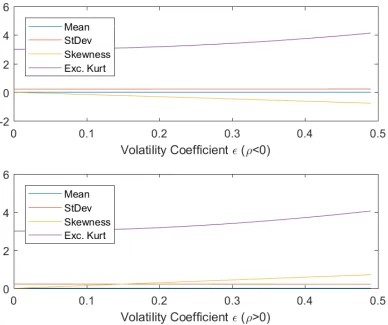
5.31 Mean, standard deviation, skewness and kurtosis of the Heston model varying the volatility coefficientε . . . 136
5.32 Movie comparing the Euler and the exact scheme. . . 139
5.33 Movie of simulated log-returns in the Heston model. . . 140
5.34 Movie of simulated variance in the Heston model. . . 141
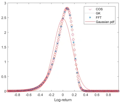
5.35 Heston vs Black-Scholes: comparing densities . . . 145
5.37 Heston PDF changing ε . . . 149
5.38 Heston PDF changingκ . . . 149
5.39 Heston PDF changing θ . . . 149
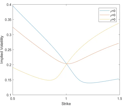
5.40 Implied Volatility as a function ofρin the Heston model . . . 150
5.41 Implied Volatility as a function ofe in the Heston model . . . 150
5.42 Implied Volatility as a function ofθ in the Heston model . . . 151
5.43 Implied Volatility as a function ofκin the Heston model . . . 151
5.44 The app can be downloaded from herehttps://sites.google.com/uniupo.it/stochasticcalculus/download-apps. Its functioning has been checked on Windows 64 bit. . . 154
6.1 ABM vs JD: sample trajectories . . . 157
6.2 Poisson, Compound Poisson and Gamma processes: sample trajectories . . . 162
6.3 Merton JD: sample trajectories . . . 170
6.4 Merton JD vs the Brownian motion: density and returns . . . 171
6.5 VG: term structure of skewness and excess kurtosis . . . 180
6.6 VG vs Brownian motion: densities . . . 181
6.7 VG process: sample trajectories . . . 182
6.8 Implied Volatility as a function ofθ in the VG model . . . 188
6.9 VG PDF changingθ . . . 188
6.10 Implied Volatility as a function ofkin the VG model . . . 188
6.11 VG PDF changingσ . . . 188
6.12 Implied Volatility as a function ofσin the VG model . . . 189
6.13 VG PDF changingk . . . 189
6.14 Convergence of L´evy processes to the Brownian motion . . . 190
7.1 Girsanov theorem: Densities and distribution under change of measure . . . 211
7.2 Girsanov theorem: simulated paths under changes of measure . . . 212
10.1 Density and Cumulative Distribution of the Gaussian random variable. . . 223
10.3 Density and Cumulative Distribution of the Lognormal random variable. . . 226
10.5 Density of the Chi-Square random variable varyingn. . . 228
10.4 Density and Cumulative Distribution of the Chi-Square random variable withn=20 degrees of freedom. . . 229
10.6 Density and CDF of the noncentral chi-squared distribution withn=5 andd=2. . . 231
10.7 Density of the non-central chi-square distribution varying the parameter of non centralityd. . . 232
10.8 Density and CDF of the Poisson distribution with λ=5 . . . 234
10.9 PDF (top) and CDF (bottom) of the Poisson distribution varying the rate of arrivalλ. . . 235
10.10Density and CDF of the Exponential distribution withλ=1.5. . . 237
10.11Density and CDF of the Gamma distribution with α=5,λ=0.5. . . 239
10.12PDF and CDF of the Gamma distribution varying the shape parameterα and the rate parameterλ . . . 240
10.13Bivariate standard Gaussian distribution and contour levels. ρ=0.9 . . . 245
10.14Bivariate standard Gaussian distribution and contour levels. ρ=0.0 . . . 246
10.15Bivariate standard Gaussian distribution and contour levels. ρ=−0.9 . . . 247
10.16Jointly simulated standard Gaussian random variables with different correlation . . . 248
10.17Gaussian margins, non Gaussian joint distribution . . . 250
10.18Non Gaussian convolution . . . 250
10.19Inverse transform method for a hypothetical CDF FX. . . 251
10.20Sampling from the standard Gaussian distribution. . . 253
10.21Sampling from the Gaussian distribution with µ=0.2 andσ =0.1. . . 254
10.22Sampling from the Lognormal distribution with parametersµ =0.05 andσ=0.2. . . 255
10.23Sampling from the Poisson distribution with λ=10. . . 257
10.24Sampling from the Gamma distribution with α=2,λ=0.5. . . 258
10.25Sampling from the bivariate Gaussian distribution (positive correlation). . . 261
11.1 Left: Rectangle rule, Right: Mid-point. . . 265
11.2 Approximation of the integral using trapezium. . . 266
11.3 Matlab adaptive routine quad: integration ofsin(1/x) . . . 274
12.1 Black–Scholes price–FFT price . . . 290
2.1 Calculus withdW . . . 24
3.1 Properties of the stochastic integral. . . 33
3.2 Properties of the arithmetic Brownian motion process. . . 38
3.3 Examples of deterministic and stochastic differential equations. . . 45
5.1 Relevant SDEs for Financial Modelling . . . 60
5.2 Properties of the geometric Brownian motion process. . . 64
5.3 Light Sweet Crude Oil (WTI) Futures prices quoted at CME as of march 12, 2013 . . . 72
5.4 Monte Carlo simulation: Futures prices . . . 74
5.5 Properties of the Vasicek model . . . 84
5.6 Properties of the Square-Root model . . . 102
5.7 Moments of log-returns in the CEV model varying the leverage parameterβ. . . 113
5.8 Properties of the Constant Elasticity of Variance CEV(µ,σ,β) . . . 115
5.9 Moments of the Heston model . . . 132
5.10 Moments computation by inversion of the characteristic function in the Heston model . . . 144
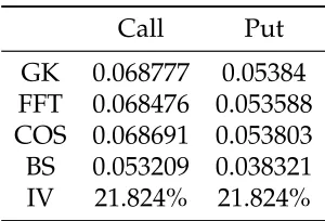
5.11 Prices of European at-the-money call and put options in the Heston model . . . 147
5.12 Properties of the Heston model. . . 153
6.1 Properties of the Gamma process. . . 161
6.2 Sample moments of daily log-price changes in oil price in year 2012. . . 167
6.3 Calibrated parameters of the MJD model to sample moments of daily log-price changes in oil price for year 2012. 168
6.4 Properties of the Merton Jump-Diffusion model. . . 172
10.1 Probability intervals of the Gaussian distribution. . . 222
10.2 Moments of the Gaussian distribution. . . 222
10.3 Properties of the Lognormal distribution. . . 225
10.4 Moments of the Chi-square distribution. . . 228
10.5 Moments of the noncentral chi-squared distribution. . . 231
10.6 Moments of the Poisson distribution. . . 233
10.7 Moments of the Exponential distribution. . . 236
10.8 Moments of the Gamma distribution. . . 239
11.1 Numerical integration of the integral in 11.7. . . 270
11.2 Numerical integration error in the computation of the integral in 11.7 using different rules. . . 270
11.3 Comparing quadrature methods . . . 271
11.4 Trapezoid Rule: Estimate of the order of convergence . . . 271
11.5 Numerical integration of the integral in 11.7. . . 276
11.6 Numerical integration error in the computation of the integral in 11.7 using different rules. . . 276
11.7 Comparing quadrature methods . . . 277
11.8 Gauss-Legendre integration with 5 points . . . 278
11.9 Numerical Integration of the function 11.7 usign a Gauss-Legendre rule . . . 279
11.10Syntax of the MATLAB adaptive quadrature routines. . . 279
12.1 Elementary properties of the characteristic function. . . 282
12.2 Pseudo-code for option pricing via the FFT algorithm. . . 287
12.3 Merton Jump Diffusion distribution: COS approximation . . . 301
1. To introduce the concept of Brownian motion.
• WhatW(t)anddW(t)are; • What the properties ofW(t)are.
2. Explaining the meaning of the stochastic differential equation
dX=µ(X,t)dt+σ(X,t)dW(t). 3. Explaining the meaning of the stochastic integral, specifically
• To give a meaning to
X(T) = X(0) +
Z t
0 µ(Xs,s)ds +
Z t
0 σ(Xs,s)dWs; • Properties ofX(T) : distribution, expected value, variance.
• How to construct a (continuous) martingale.
4. Explaining the Ito’s formula.
• For example, how to relate
to
dlnS=
µ−σ
2
2
dt+σdW 5. Examples of common stochastic differential equations.
• Arithmetic Brownian Motion; • Geometric Brownian Motion;
• Mean-Reverting Gaussian Model (Vasicek); • Mean-Reverting Square-Root Model (CIR); • Constant Elasticity of Variance Model (CEV); • Stochastic Volatility Model (Heston);
6. Examples of jump processes.
• Poisson Process;
• Poisson Compound Process; • Gamma Process;
• Jump Diffusion Process (Merton );
• Jump Diffusion Process (Kou double exponential);
Contents
2.1 Defining the Brownian Motion . . . 10
2.1.1 The odd properties of the Brownian Motion . . . 10
2.1.2 Density of the Brownian Motion at different Time Horizons . . . 11
2.1.3 The (auto)-covariance function . . . 12
2.1.4 Correlated Brownian motions . . . 13
2.1.5 Martingale property . . . 14
2.1.6 Scaling property . . . 15
2.1.7 Markov property . . . 16
2.1.8 Simulation of Brownian sample paths . . . 17
2.1.9 Total Variation . . . 17
2.1.10 Quadratic Variation . . . 19
2.1.11 Properties of the Increments of the BM . . . 23
In this chapter we define the Brownian Motion (BM) and we will present its main properties. Let us recall that a stochastic process (s.p.) is a family of indexed random variables (r.v.’s). Usually, but it is not necessary, the index refers to time. If we use the time index, as we will do, this means that at each instant of time (if the stochastic process is continuous in time) or at discrete times (if the stochastic process is discrete in time) we have to draw a r.v.. Once we have extracted them, we observe a path or a trajectory of the s.p.. We have to stress that in order to fully characterize the s.p. we have to specify the distribution of the r.v. at different times as well as their time dependence properties, i.e. how the r.v. that will be extracted in 1 month will affect the value of the r.v. that will be extracted in 2 months. The simplest process in continuous time is the Brownian motion.
A comprehensive introduction to the BM, stochastic differential equations and and their properties with a range of financial applications is provided by the book of S. Shreve Stochastic Calculus for Finance II, Springer Finance, 2004.
2.1. DEFINING THEBROWNIANMOTION
Fact 1 (Brownian Motion) The stochastic process W :={W(t) : t≥0}is called Brownian motion if i) W(0) = 0
ii) for s≤t, W(t)−W(s)is independent of the past history of W until (and including) time s, i.e. the Brownian motion has increments which are independent of theσ−algebraF(s)generated by the process up to time s.
iii) for0≤s≤t, W(t)−W(s)and W(t−s)have the same distribution, which is Gaussian with mean zero and variance(t−s), i.e. W(t)−W(s) ∼W(t−s) ∼ N(0,t−s).
In other words. the Brownian motion has stationary increments.
iv) W has continuous sample paths: W(t), t≥0is a continuous functions of t (a.s.). 2.1.1. THE ODD PROPERTIES OF THEBROWNIANMOTION
• W(t)is not monotone in any interval, no matter how small the interval is (like in a fractal structure). This property means that, even over very small time intervals, we cannot say if the BM is increasing or decreasing.
• W(t)is nowhere differentiable. This property means that we cannot predict the movement of the BM over the next time interval.
• W(t)is a process of unbounded variation, i.e. the space it travels over any finite time period is infinite. This property is a consequence of the two previous properties. BM paths are so irregular that if you try to measure their length you do not obtain a finite measure.
• W(t)is a process of bounded quadratic variation. Quadratic variation, as we will see shortly, is connected to the variance of the process. Therefore, even being a very irregular process, BM at each finite time has a finite variance.
• Brownian motion has the Markov property. Broadly speaking, this means that the information we have on the past paths of a BM is not useful in determining the current value of the process.
• E(W(t)W(s)) = min(s,t). This property, discussed later, is telling us that the time dependence of the Brownian motion depends on what happened up to min(s,t).
• The BM will eventually hit any and every real value no matter how large, or small. The BM paths are so dispersed that the BM can reach any desired level in finite time with positive probability.
• Once a BM hits a value, it immediately hits it again infinitely often.
2.1.2. DENSITY OF THE BROWNIANMOTION AT DIFFERENTTIME HORIZONS
Fact 2 (Density function of the Brownian Motion) From the definition it follows that W(t)−W(s) ∼ N(0,t−s).
and therefore the density function of the increment of the BM between time s>0and time t>s is
φ0,√t−s(x) = p 1
2π(t−s)
exp −1 2
x
√
t−s
2!
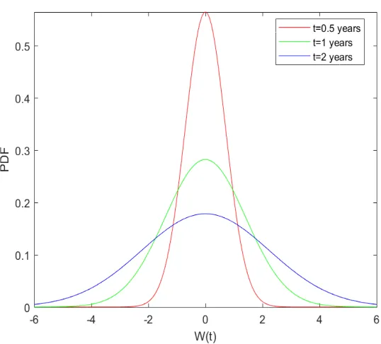
Figure 2.1:Density of the Brownian Motion at different time horizons.
Remark 3 We observe that W(t) = W(t)−W(0), from which it follows that W(t)∼ N(0,t). The dispersion of the BM, as measured by the variance, increases with the time horizon t. This is shown in Figure (2.1).
2.1.3. THE(AUTO)-COVARIANCE FUNCTION
• The (auto)-covariance function of a stochastic processXhaving expectationµXis defined as
• The variance function of X is justcX(t,t).
Fact 4 (Covariance function of the Brownian Motion) A Brownian Motion has covariance function given by cW(t,s) = min(t,s).
Proof: The (auto)-covariance function of the BM
• Let us consider two time instants,tands, t<s. We have
cW(t,s) = cov(W(t),W(s))
= cov(W(t),(W(s)−W(t)) +W(t))
= cov(W(t),(W(s)−W(t))) +cov(W(t),W(t)) = 0+cW(t,t)
= t,
where the penultimate equality follows from the definition of BM.
• With a similar reasoning, if we taketandswith s<t, we have
cW(t,s) =s.
• Therefore
cW(t,s) = min(t,s).
2.1.4. CORRELATEDBROWNIAN MOTIONS
Proposition 5 In order to construct two Brownian motions, W(t)and X(t), such that
we may take
W(t) = ρX(t) + q
1−ρ2Z(t),
where Z(t)is another Brownian motion independent of X(t).
To see this we note the following.
• Any process of the formW(t) = aX(t) +bZ(t)possesses the stationary, independent increments property, has continuous sample paths and starts from 0 at timet.
• The distribution ofW(t) = aX(t) +bZ(t)isN 0,(a2+b2)t
.
• Choosinga =ρ,b =p1−ρ2implies thatVar(W(t)) = t, so thatW(t)is a standard Brownian motion. • Further
Cov(W(t),X(t)) =Cov(ρX(t) + q
1−ρ2Z(t),X(t)) =ρVar(X(t)) = ρt.
2.1.5. MARTINGALE PROPERTY
Remark 6 A stochastic process X = (X(t) : t≥0)is a martingale with respect to the probability measurePif the following conditions are satisfied.
i) E|X(t)|<∞for all t ≥0;
ii) E[X(t)|F(s) ] =X(s)for all s ≤t.
• In other words, a martingale is a random process whose future variations are completely unpredictable given the current information set.
• For this reason, the best forecast of the change inXover an arbitrary interval is zero, i.e. E[X(t)−X(s)|F(s) ] =0.
• A martingale represents a fair game: given the knowledge we currently have, on average the return produced by the investment is what we invested in it.
Proof: The martingale property of the BM
We check that the Brownian motion satisfies the two properties of a martingale process. Hence.
• For the first property, direct calculations show us
E|W(t)| =
Z 0
−∞
−y
√ 2πt
exp −1 2 y √ t 2! dy+ Z ∞ 0 z √ 2πt
exp −1 2 z √ t 2! dz = 2 Z ∞ 0 z √ 2πt
exp −1 2 z √ t 2! dz = r 2t
π <∞.
• Let us consider two time instants,sandt, s<t. We have
E[W(t)|F(s)] =E[W(t)−W(s) +W(s)|F(s)] =E[W(t)−W(s)] +W(s) =W(s), where the last two equalities follow from the definition of BM.
2.1.6. SCALING PROPERTY
Fact 8 (Scaling Property) Let c>0and W(t)a Brownian motion. Then the process B(t) = W(ct)/√c is a Brownian motion.
Proof: The scaling property of the BM
We check that the processB(t)satisfies the definition of Brownian motion. Indeed it starts from zero and it is Gaussian; further. • The moments are.
E(B(t)) = E(W(ct))/√c=0
• Finally, the processB(t)has independent and stationary increments due to again the fact thatW(t)is a Brownian motion. Remark 9 We can rewrite the scaling property given above as √cB(t) = W(ct). Intuitively, this relation suggests that rescaling a Brownian motion by a positive constant is equivalent to observing the Brownian motion evolving according a rescaled time. The expression W(ct), in fact, shows that the process W does not evolve according to the traditional calendar clock t, but a rescaled clock ct. The bigger c, the faster the rescaled clock, the bigger the variance of√cB(t).
We will discuss in further details the change of clock from t to a rescaled version later in relation to solving stochastic differential equations. Indeed, the above result is a particular case of the Dambis, Dubins-Schwarz Theorem given in section 3.6.
2.1.7. MARKOV PROPERTY
Remark 10 LetF (s) denote theσ−field generated by the process up to time s.The process{X}t≥0has the Markov property if, for t ≥ s,
the conditional distribution of X(t)givenF (s)is the same as the conditional distribution of X(t)given X(s)
P(X(t) ≤y|F (s)) =P(X(t)≤y|X(s)), a.s. • In practice, this means the process does not remember how it got to the current statex. Fact 11 (Markov Property) Brownian motion has the Markov property.
2.1.8. SIMULATION OFBROWNIAN SAMPLE PATHS
In order to simulate a Brownian motion sample pathW(t)on the interval[0,T]we can adopt the following steps. 1. Choose an integernand let∆t= Tn, so thatti =i∆t, fori=0, 1, . . . ,n.
2. Generate a sequenceε1, . . . ,εn of iid standard normal rvs:
(a) Generate a sequenceU1, . . . ,Unof Uniform r.v.’s in the interval(0, 1);
(b) Set εi =Φ−1(Ui), whereΦ−1(x)is the inverse cumulative distribution of the standard Gaussian distribution;
(c) SetdWi =εi
√ ∆t.
3. Finally recursively construct the sample path of the BM letting
• W(0) =0
• W(ti) =W(ti−1) +dWi, i=1, . . . ,n
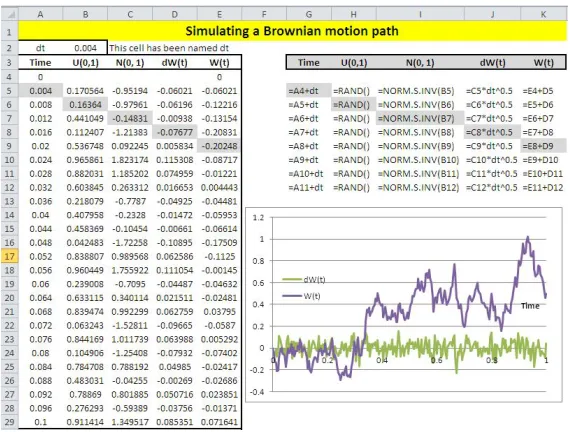
Remark 12 Notice that the simulation of the BM as described above is convenient if you are using a spreadsheet or programming language like C, VBA. This is illustrated in Figure (2.2). If you are using Matlab a different approach, avoiding for cycles, is preferred, see Figure (2.3) and the accompanying code.
A movie showing simulated paths of the Brownian motion is shown in figure 2.4.
2.1.9. TOTALVARIATION
• Given a partition of the interval [x0,xn], the variation of a function f(x) measures the total amount of up and down
movements, i.e.
TV(f) =
N
∑
i=0Figure 2.2:Simulating the Brownian Motion: Excel example.
• The notion of unbounded variation plays an important role in stochastic calculus since the majority of continuous time stochastic processes used to represent asset prices have trajectories with unbounded variation i.e. they are very irregular.
• Heuristically, functions of bounded variation are not excessively irregular. In fact, any smooth function will be of bounded variation.
Fact 13 (Total Variation of the Brownian Motion) The Brownian Motion has unbounded total variation, i.e. TV(W) =
N
∑
i=1|∆W(ti)| → ∞
Matlab Code
%%%%%%%%%%%%%%%%%%%%%%%%%%%%%%%%%%%%%%%%%% %%%%SIMULATING THE BROWNIAN MOTION%%%%%%%% %%%%%%%%%%%%%%%%%%%%%%%%%%%%%%%%%%%%%%%%%%
nsimul=50; %Assigning the number of simulated paths
expiry=1; %time to maturity (expiry)
nsteps=250; %number of steps
dt=expiry/nsteps;%time step (dt)
timestep=[0:dt:expiry]';%observation times (timestep) %Simulate increments of the BM setting:
dw=randn(nsteps,nsimul) * dtˆ0.5;
%Simulate Brownian motion process: %use cumulative sum of the increments
cdW=[zeros(1,nsimul); cumsum(dw)];
%Plot simulated paths:
h=figure('Color', [ 1 1 1]); plot(timestep, cdW) title('Simulated Paths of the Wiener Process'); xlabel('Time (years)')
%Save the figure in a png format
print(h,'−dpng','FigBMPaths')
Figure 2.3:Simulated Paths of the Brownian Motion.
2.1.10. QUADRATIC VARIATION
• Quadratic variation is linked to the variance of the process.
• Given a partition of the interval[t0,tn], the quadratic variation of a function f(t)is given by
QV(f) =
N
∑
i=0(f (ti)−f (ti−1))2.
Figure 2.4:Movie of simulated variance in the Heston model.
• For example, consider the functionX(t) = at. This function has QV equal to∑iN=1(a∆ti)2 = a2N∆t2 = a2N(Nt )2 → 0 as
Fact 14 (Quadratic Variation of the Brownian Motion) The quadratic variation of the BM over the time interval[0,t]tends to t QV(W) =
N
∑
i=1(∆W(ti))2 →t
as N →∞where t0,t1, ...,tN represents a discrete partition of the interval[0,t].
Total Variation and Quadratic Variation of the BM: Matlab example
• Figures (2.5) illustrate, by simulation, that:
– the Total Variation of the BM grows unbounded as we refine the partition of the interval (0,1). Notice that given
E|dW(ti)| = r
dt2
π,
so that (given thatdt =t/N)
E(TV) = N
r
dt2
π = r
TN2
π,
that diverges as we increase the number of points of the partition, for a given horizonT. The blue line in the left panel represents the expected value of the total variation and its simulated values (in red) as the number of points in the partition increases.
– the Quadratic Variation converges to the length of the interval as we refine the partition of the interval (0,1). In this case, it is easy to show that the expected value of the Quadratic Variation converges toT as we increaseN.
• The Matlab code to generate these figures is as follows.
Figure 2.5:Left: the Brownian motion has unbounded total variation. Right: the Brownian motion has bounded quadratic variation
%%%%%%%%%%%%%%%%%%%%%%%%%%%%%%%%%%%%%%%%%%%%% %%%COMPUTING BY SIMULATION TOTAL VARIATION%%% %%%AND QUADRATIC VARIATION OF THE BM%%%%%%%%% %%%%%%%%%%%%%%%%%%%%%%%%%%%%%%%%%%%%%%%%%%%%%
clear all;
i=1; %Counter to be used in the for cycle
expiry=1; %Time horizon
nsimul=500;%Number of simulations
N=(50:50:10000);%number of points in the partition
for jstep=N %increase the number of steps (refine the partition)
dt=expiry/jstep; %reduce the time step %simulate increments of the BM
%compute total variation
TV(i,:)=sum(abs(dW));
%compute quadratic variation
QV(i,:)=sum(dW.ˆ2); i=i+1; %update the counter
end
h=figure('Color',[1 1 1]); plot(N, TV,'r')
hold on
plot(N,(N*expiry*2/pi).ˆ0.5,'b') %this is the plot of the E[TV]
title('BM has unbounded total variation');
xlabel('Number of steps (Fixed time interval=1yr)') print(h,'−dpng','LecBM fig TV')
h = figure('Color',[1 1 1]); plot(N,QV,'r',N,expiry,'b.')
legend('Simulated QV', 'Theoretical QV') title('BM has bounded quadratic variation');
xlabel('Number of steps (Fixed time interval=1yr)')
2.1.11. PROPERTIES OF THE INCREMENTS OF THEBM
In the following we set equal to 0 quantities that areo(dt), i.e. that tend to zero faster than dt. Further, we read the quantity ‘dW(t)’ as the infinitesimal increment of the Brownian motion (i.e. the increment of the process over an infinitesimal period of timedt).
Fact 15 (Calculus with dW) We have 1. dW(t) ∼ N(0,dt) (by definition);
2. E(dW(t)) =0; (by definition);
4. E dW2(t) =dt;(this is the second moment of the increment of the BM: i.e. its variance as the mean is zero by definition); 5. Var dW2(t)
=Et dW4(t)−Et dW2(t)2 =3dt2−dt2 =o(dt);(as dW is Gaussian);
6. dW2(t) =dt (it follows by properties (4) and (5)); i.e. the square of the increment can be approximated by its mean value as the error of doing so, which is measured byVar dW2(t)
is negligible. 7. E(dW(t)dt)2=E dW2(t)
dt2 =dt3 =o(dt)it follows by (4); 8. Var(dW(t)dt) = E(dW(t)dt)2−E((dW(t)dt))2 =E dW2(t)
dt2−o(dt) = o(dt);
9. dW(t)dt =o(dt)(it follows by (3) and (8): the argument is the same as for point (6) above). 10. We can summarize the above results by using Table (2.1).
× dt dW(t)
dt 0 0
dW(t) 0 dt
Contents
3.1 Introduction . . . 26 3.2 Defining the Stochastic Integral . . . 26 3.3 The Ito stochastic integral as a mean square limit of suitable Riemann-Stieltjes sums . . . 27 3.4 A motivating example: ComputingR0tW(s)dW(s). . . 28
3.4.1 Example: ComputingR0tW(s)dW(s)by simulation . . . 28
3.5 Properties of the Stochastic Integral . . . 28 3.6 Stochastic integrals as Time Changed Brownian Motions . . . 32 3.7 Ito process and Stochastic Differential Equations . . . 36 3.8 ABM with deterministic volatility . . . 36
3.8.1 Matlab: Simulating the Arithmetic Brownian Motion . . . 39
3.9 Solving Stochastic Integrals and/or Stochastic Differential Equations . . . 42
3.9.1 Deterministic vs. Stochastic Differential Equations . . . 43 3.9.2 Examples of stochastic differential equations . . . 45 3.9.3 Existence and uniqueness of the solution . . . 45
3.1. INTRODUCTION
• The Ito or Stochastic integral is one way of defining sums of uncountable and unpredictable random increments over time:
Z T
0 σ(X(s),s)dW(s)
| {z }
sum of iid noises
≈
n−1
∑
j=0σ X tj
,tj
| {z }
vol scaling factor intj
W tj+1
−W tj
| {z }
noise in[tj,tj+1] .
• Recall that the sample paths of BM are nowhere differentiable and have unbounded variation.
• This has major consequences for the definition of a stochastic integral with respect to Brownian sample paths.
Fact 16 (Problem in defining the stochastic integral) IfR0T f (s)dg(s) exists as a Riemann-Stieltjes integral for all continuous func-tions f on[0,T], then g necessarily has bounded variation. Unfortunately, the BM has unbounded variation.
3.2. DEFINING THESTOCHASTIC INTEGRAL
• Last observation is telling us that if our aim is to define the stochastic integralR0T f (s)dW(s)for all continuous determin-istic functions f on[0,T], the pathwise integration suggested by the Riemann-Stieltjes integral approach fails since it does not allow the integration of a large class of integrable functions f.
• We will define the integral as a probabilistic average. This will lead us to the so called Ito stochastic integral.
• We define the Ito stochastic integral as a mean square limit of suitable Riemann-Stieltjes sums. This is equivalent to say that the variance of the random errorεn =Xn−X, goes to zero as we refine the partition.
• This has the disadvantage that we loose the intuitive interpretation of an integral which is naturally provided by a pathwise integral.
Definition 17 (Mean square convergence) Let us consider a sequence of random numbers X1,X2, . . . ,Xn, . . .with Xn ∈ L2i.e.E X2n
< ∞. We say that the sequence of r.v. Xnconverges in mean square to the random variable X, and we write Xn L
2
→X, ifflimn→∞E |Xn−X|2
3.3. THEITO STOCHASTIC INTEGRAL AS A MEAN SQUARE LIMIT OF SUITABLERIEMANN-STIELTJES SUMS
• Let:
1. σ(u)is an adapted process1; 2. σ(u)is square integrable, i.e. E
RT
0 σ2(u)du
<∞.
• Then the following limit
lim
kΠk→0
n
∑
j=1σ tj−1 W tj
−W tj−1
= Iσ(0,T)
exists (in the mean square sense) and is independent of the partitions used to take the limit.
• By definition, this limit is the Ito integral ofσ(t)with respect to BM over[0,T].
Example 18 Let us consider the Ito integral of the identity function with respect to BM over[0,T]. Given a partitionΠ={0=t0 <t1 < ...<tn−1 <tn =t}, we define the Riemann-Stieltjes sums
Sn = n
∑
j=1(W(tj)−W(tj−1)).
As Sn is a telescopic sum, then Sn =W(T), therefore Z T
0 dW(u) =W
3.4. A MOTIVATING EXAMPLE: COMPUTING R0tW(s)dW(s)
• Given a partitionΠ ={0=t0<t1 <...<tn−1<tn =t}, let us define the Riemann-Stieltjes sums:
Sn = n
∑
j=1W(tj−1)(W(tj)−W(tj−1)).
• Using the binomial formula for(W(tj)−W(tj−1))2,Sn can be written as:
Sn = W
2(t) 2 −
1 2
n
∑
i=1(W(tj)−W(tj−1))2 =
W(t) 2 −
1
2QVn(W)(t). • But if we refine the partitionτn, thenQVn(W)(t) →t, so that
Var
Sn−W
2(t)−t 2
→0,
i.e. Sn converges in mean square to W
2(t)−t
2 , which we can take as the value of the integral
Rt
0W(s)dW(s).
3.4.1. EXAMPLE: COMPUTING R0tW(s)dW(s) BY SIMULATION
The following code illustrates the one-to-one relationship betweenRt
0W(s)dW(s)and its value
W2(t)−t
2 . See also Figure (3.1): the blue line in the plot has a unit slope and goes trough the origin. This confirms, by simulation, that the integral, albeit being a random variable, can be written as W2(2t)−t.
3.5. PROPERTIES OF THESTOCHASTIC INTEGRAL
%%%%%%%%%%%%%%%%%%%%%%%%%%%%%%%%%%%%%%%%%%%% %%%Computing Integral[W(s) dW(s),{s,0,T}]%%% %%%%%%%%%%%%%%%%%%%%%%%%%%%%%%%%%%%%%%%%%%%%
clear all; expiry=1; nstep=10000; nsimul=10;
%fix the time step
dt=expiry/nstep;
%simulate increments of the BM
dW=randn(nstep,nsimul)*dtˆ0.5;
%simulate the BM by cumulating the increments
W=[zeros(1,nsimul); cumsum(dW)];
%Approximated value of the stoch. integral by a sum
StocInt=sum(W(1:end−1,:).*dW)';
%Exact Value
ExactInt=(W(end−1,:).ˆ2−expiry)'/2;
%Plot the result:
%The simulated values stay on the 45 degree red line.
h = figure('Color',[1 1 1]); axis equal
plot(StocInt, ExactInt,'.') hold on
fplot(@(x) x,[−1,6],'red') ylabel('\int 0ˆt W(s)dW(s)')
print(h,'−dpng','FigStocIntegral') Figure 3.1:Computing by simulation the stochastic integral Rt
0W(s)dW(s)
and comparing to its value W(t2)2−t.
1. E[Iσ(0,T)] =0.
2. E
Iσ2(0,T)
=EhRT
0 σ2(u)du
i
3. The Itˆo integral is Gaussian, for any deterministic integrand functionσ(t)
Iσ(0,T)∼ N
0,
Z T
0 σ
2(u)du
.
4. Iσ(0,T)is aP-martingale.
5. The QV of Iσ(0,T)over the time interval[0,T]is
QV(Iσ) = N
∑
i=1σ2(ti−1) (W(ti)−W(ti−1))2 →
Z T
0 σ
2(u)du
as N →∞.
Proof: Properties of the Stochastic Integral
The above mentioned properties can be shown using the definition of Brownian motion, the fact that the integrand function is an adapted process and the properties listed in section 2.1.11.
1. We use the Tower property of the conditional expectation, so that
E[Iσ(0,T)] = Z T
0 E
[σ(u)dW(u)] =
Z T
0 E[Eu(σ(u)dW(u))] =
Z T
2. Given a partitionΠ =0 =t0<t1<... <tn−1 <tn =t, consider the Riemann-Stieltjes sums
Sn = n
∑
j=1σ(tj−1)(W(tj)−W(tj−1)). It follows
S2n = n
∑
j=1σ2(tj−1)(W(tj)−W(tj−1))2+
∑
j i
∑
6=jσ(tj−1)σ(ti−1)(W(tj)−W(tj−1))(W(ti)−W(ti−1)). Without loss of generality, assumeti <tj; we note
ES2n = E
" n
∑
j=1Etj−1
σ2(tj−1)(W(tj)−W(tj−1))2
#
+E
"
∑
j i
∑
6=jEtj−1 σ(tj−1)σ(ti−1)(W(ti)−W(ti−1))(W(ti)−W(ti−1))
# = E " n
∑
j=1σ2(tj−1)(tj−tj−1)
#
where the last equality follows from the definition of Brownian motion. The result follows.
3. If the integrand function is deterministic, the stochastic integral turns out to be a weighted sum of (independent) Gaussian increments, and therefore it is Gaussian as well. The mean and the variance of the stochastic integral follows from the above properties.
4. We note that Iσ(0,T) = Iσ(0,t) +Iσ(t,T). Then
Et[Iσ(0,T)] = Iσ(0,t) +Et[Iσ(t,T)]
= Iσ(0,t) +Et Z T
t Eu(σ(u)dW(u))
5. Given a partition of the interval[0,T], by definition the QV of the process Iσis given by
QV(Iσ) = N
∑
i=1(Iσ(0,ti)−Iσ(0,ti−1))2
=
N
∑
i=1σ2(ti−1) (W(ti)−W(ti−1))2 →
Z T
0 σ
2(u)du.
Remark 20 As the Ito integral is a zero mean process, the Ito isometry implies that
Var(Iσ(0,T)) =E Z T
0 σ
(u)2du
.
Why is this result relevant in finance? It is related to the interpretation of the implied volatility of an option as the average variance of the underlying stock return over the remaining life of the option.
3.6. STOCHASTIC INTEGRALS AS TIME CHANGED BROWNIANMOTIONS
The following result provides the equivalent for stochastic integrals of the scaling property that we have seen to apply to the Brownian motion (Section 2.1.6).
In order to simplify notation let us denote the QV over the period [0,t] of a stochastic processXas [X]t =QV(X).
IMPORTANT PROPERTIES OF THE STOCHASTIC INTEGRAL
Iσ(0,t)is a stochastic process with continuous sample paths.
Iσ(0,t)is a martingale wrt to the Brownian filtration.
Iσ(0,t)has zero expectation
E(Iσ(0,t)) = 0.
Iσ(0,t)satisfies the isometry property:
Var(Iσ(0,t)) = E h
Rt
0 σ2(u,w)du
i
. For constantsαand β, Iσ(0,t)is linear
Iασ1+βσ2(0,t) = αIσ1(0,t) +βIσ2(0,t). and for adjacent intervals 0≤t≤ T
Iσ(0,T) = Iσ(0,t) +Iσ(t,T).
An intuitive argument for the Dambis, Dubins-Schwarz Theorem
• We have seen in Fact 19 that a continuous martingale can be written in terms of the stochastic integral
Z t
0 σ(u)dW(u). • Also, it follows from Fact 19 that
Z
σ(u)dW(u)
t
=
Z t
0 σ
2(u)du (It ˆo isometry)
• According to the Dambis, Dubins-Schwarz Theorem given above, there exists a Brownian motionWsuch that
Z t
0 σ(u)dW(u) =W
Z t
0 σ
2(u)du
.
Note that the two Brownian motions entering both side of the previous equations are not the same; this is a slight abuse of notation.
• Indeed, letM(t) =WR0tσ2(u)du
. Then, the properties of the Brownian motion imply
Et(M(t)) =Et
W
Z t
0 σ
2(u)du
=0,
from which it follows thatE(M(t)) =0.
• Further, the properties of the Brownian motion also imply
Vart(M(t)) =Vart
W
Z t
0 σ
2(u)du
=
Z t
0 σ
2(u)du;
consequentlyVar(M(t)) =ER0tσ2(u)du
• Finally, consider two points in times <t. Then
Es(M(t)) = Es(M(t)−M(s)) + M(s)
= Es Et W Z t 0 σ 2(
u)du
−W
Z s
0 σ 2(
u)du
+M(s) = M(s)
where the second equality follows from the Tower property (or law if iterated conditional expectations), and the last equality follows from the fact that the increments of the Brownian motion have zero mean. Hence the process M(t) is a martingale.
The meaning of the Dambis, Dubins-Schwarz Theorem is the following. • LetT(t) = [M]t.
• In analogy with what observed for the scaling property of the Brownian motion in Section 2.1.6, we can interpret the stochastic integral R0tσ(u)dW(u) as a Brownian motion evolving on a time scale which is not governed by the standard calendar clock, but by a stochastic clockT(t), i.e.WR0tσ2(u)du
.
• Thus, if we model prices using a stochastic integral, implicitly we recognize that price changes are random due to two reasons.
• Firstly, there is uncertainty related to the time at which the next investor enters the market placing a transaction which is going to alter the current level of the prices.
• Secondly, there is uncertainty related to the magnitude of the change.
• T(t)models the first effect. The Brownian motionWmodels the second one. • In Finance the processT(t)is referred to as business time.
3.7. ITO PROCESS AND STOCHASTICDIFFERENTIAL EQUATIONS
Fact 22 An Ito process is a stochastic process of the form X(t) = X(0) +
Z t
0 f
(X(u),u)du+
Z t
0 σ
(X(u),u)dW(u),
where X(0)is a random variable, and f (X(t),t),σ(X(t),t)are adapted processes satisfying some regularity conditions. The Ito processX(t)can also be written in differential form (as a shorthand notation)
dX(t) = f (X(t),t)dt+σ(X(t),t)dW(t),
X(0) = X. Meaning of f (X(t),t)andσ(X(t),t)
• We observe that
Et(dX(t)) = f(X(t),t)dt,
Vart(dX(t)) = σ2(X(t),t)dt, hence, we can interpret
– f(X(t),t)dt as the expected instantaneous change in X over the time period (t,t+dt); f (X(t),t) is called DRIFT COEFFICIENT.
– σ2(X(t),t)dtas the variance of the instantaneous changes;σ(X(t),t)is calledDIFFUSION COEFFICIENT. 3.8. ABMWITH DETERMINISTIC VOLATILITY
• An Arithmetic Brownian Motion is an Ito process defined as
X(t) = X(0) +
Z t
0 µ(s)ds+
Z t
for any deterministic functionsµ(t),σ(t)such thatR0Tσ2(u)du <∞for any fixedT <∞. • In virtue of the properties of the stochastic integral, it follows that
X(t) ∼ N
X(0) +
Z t
0 µ(s)ds,
Z t
0 σ
2(s)ds
.
• The conditional distribution of X(t) givenF (s)is
X(t)|F (s)∼ N
X(s) +
Z t
s µ(s)ds, Z t
s σ
2(u)du
.
• The expressions of the variance obtained above are obtained using theIto isometry.
• The corresponding stochastic differential equation is
dX(t) =µ(t)dt+σ(t)dW(t).
Example 23 Let us assume thatµ(t) = µ ∈Randσ(t) =σ >0, then the ABM is given by
X(t) = X(0) +µt+σW(t),
or, equivalently
dX(t) =µdt+σdW(t).
ARITHMETICBROWNIAN MOTION: FACTS
The SDE
dX(t) = µdt+σdW(t),X(0) = x0. The solution
X(t) = X(0) +µt+σW(t). The distribution ofX(t)
X(t)∼ N X(0) +µt,σ2t. The moments ofX(t)
E0(X(t)−X(0)−µt)p= (σp(t))p(p−1)!!ifpis even. In particular:
ifn =1 E0(X(t)) =X(0) +µt.
ifn =2 E0 X2(t)
= (X(0) +µt)2+σ2t. The auto-covariance of X(t)
3.8.1. MATLAB: SIMULATING THEARITHMETIC BROWNIANMOTION
Sample paths of the ABM are presented in Figure (3.2) (see the accompanying code below). Figure (3.6) shows the distribution of the ABM at different time horizons.
Matlab Code
%%%%%%%%%%%%%%%%%%%%%%%%%%%%%%%%%%%%%%%%%%%%%%%%%%%%%%%% %%%%SIMULATING THE ARITHMETIC BROWNIAN MOTIONS%%%%%%%%%% %%%%%%%%%%%%%%%%%%%%%%%%%%%%%%%%%%%%%%%%%%%%%%%%%%%%%%%%
clear all
%Assign the number of simulated paths (nsimul)
nsimul=10000;
%Time to maturity (expiry)
expiry=1;
%number of steps (nsteps)
nsteps=250;
%time step (dt) and observation times (timestep):
dt=expiry/nsteps;
timestep=[0:dt:expiry]';
%model parameters
mu=0.2; sigma=0.3;
%Simulate increments ABM dX:
dX=mu*dt+sigma*randn(nsteps,nsimul)*dtˆ0.5;
%Simulate ABM process: cumulate increments
X=[zeros(1,nsimul); cumsum(dX)];
%compute theoretical expected value
EX=timestep*mu;
%Plot simulated paths:
h=figure('Color',[1 1 1]); plot(timestep, X)
hold on
title('Simulated Paths of the Arithmetic Brownian Process ABM(0.2, 0.3)') xlabel('Time')
print(h,'−dpng','LecBMSimulatedABM')
%Sstimate mean of X(t) from the simulations %and compare to the true one
SimulatedMean=mean(X')'; h=figure('Color',[1 1 1]);
plot(timestep, [SimulatedMean, EX]) xlabel('Time')
legend('Simulated expected value','Theoretical expected value')
title('Comparing the theoretical mean of the ABM with the one estimated via MC') print(h,'−dpng','LecBM mean ABM')
%Now we repeat the calculation for the variance. %compute theoretical variance
VX=timestep*sigmaˆ2;
%estimate variance from the simulations
SimulatedVar=var(X')'; h=figure('Color',[1 1 1]);
plot(timestep, [SimulatedVar, VX]) xlabel('Time')
legend('Simulated variance','Theoretical variance','location','best')
title('Comparing the theoretical variance of the ABM with the one estimated via MC') print(h,'−dpng','LecBM var ABM')
%We compare the simulated distribution of the process
% with the Gaussian density with the same mean and variance. %To plot the simulated distribution we use the
%new Matlab command histogram
%Plot distribution of the ABM at different dates: %Range of the plot and number of points
%Fix the times at which to plot the densities
horizon=[50, 125, 250]+1;
h=figure('Color',[1 1 1]);
for j=1:length(horizon) ndays=horizon(j);
subplot(3,1,j);
histogram(X(ndays,:),nbins,'Normalization','pdf');xlabel('ABM') hold on
plot(sort(X(ndays,:)),normpdf(sort(X(ndays,:)),EX(ndays),VX(ndays)ˆ0.5)) legend('Simulated','Gaussian','location','northwest')
xlim([bmmin, bmmax]);
title(strcat('Density in', [' ' num2str(horizon(j)/horizon(end),2)], ' years'))
end
print(h,'−dpng','LecBM dens ABM')
We also plot in a 3D diagram the time evolution of the density of the ABM, see figure 3.7.
%Assign number of bins and the edges
abmmin=mu*timestep(end)−6*sigma*timestep(end)ˆ0.5; abmmax=mu*timestep(end)+6*sigma*timestep(end)ˆ0.5; nbins=100;
edges=linspace(abmmin,abmmax,nbins);
%Build theoretical pdf at each time step
for j=2:nsteps+1
pdf values(j,:)=pdf('normal',edges,...
(mu)*timestep(j),sigma*timestep(j)ˆ0.5);
end
steps=20;
%Finally, the plot
h=figure('Color',[1 1 1]);
zlabel('Density');
title('Time evolution of the ABM density') ylim([timestep(steps) timestep(end)])
Figure 3.2:Simulated sample paths of the ABM(0.2,0.3).
Figure 3.3:Simulated and theoretical expected value of X(t) of the ABM(0.2,0.3) at different horizons.
3.9. SOLVING STOCHASTIC INTEGRALS AND/OR STOCHASTIC DIFFERENTIAL EQUATIONS
• In the previous section we have shown the equivalence between stochastic integrals and stochastic differential equations.
Figure 3.4:Simulated and theoretical variance of the ABM(0.2,0.3) at differ-ent horizons.
Figure 3.5:Simulated and theoretical standard deviation of the ABM(0.2,0.3) at different horizons.
• As illustrated in section 3.4, finding this solution can be quite complicated.
• However, there is a very useful tool for this task: Ito’s lemma. This will be introduced in the next chapter.
• In the remaining of this chapter, we want to summarize some useful facts about SDEs and their solution.
3.9.1. DETERMINISTIC VS. STOCHASTIC DIFFERENTIAL EQUATIONS
Deterministic Differential form
Figure 3.6:Simulated distribution of the ABM(0.2,0.3) at different horizons. Figure 3.7:Time evolution of the exact distribution of the ABM(0.2,0.3).
Integral form
x(t) = x(0) +
Z t
0 f (x(u),u)du
| {z }
Riemann Integral
.
Stochastic
Differential form
Integral form
X(t) =X(0) +
Z t
0 f (x(u),u)du
| {z }
Riemann Integral +
Z t
0 σ(X(u),u)dW(u)
| {z }
Stochastic Integral
. (3.2)
3.9.2. EXAMPLES OF STOCHASTIC DIFFERENTIAL EQUATIONS
Few examples of SDEs are given in Table 3.3, for which we also provide the deterministic version.
Deterministic Stochastic Name
dx=µdt dX(t) = µdt+σdW(t) Arithmetic Brownian Motion (ABM)
dx=µxdt dX(t) = µX(t)dt+σX(t)dW(t) Geometric Brownian Motion (GBM)
dX(t) = µX(t)dt+σXβ+1(t)dW(t) Constant Elasticity of Variance (CEV)
dX(t) = α(µ−X(t))dt+σdW(t) Ornstein-Uhlenbeck (Vasicek)
dx=α(µ−x)dt dX(t) =α(µ−X(t))dt+σpX(t)dW(t) Square root (Cox-Ingersoll-Ross, CIR)
dX(t) = α(µ−X(t))dt+σX(t)dW(t) Lognormal with mean-reversion
dX(t) =µX(t)dt+pv(t)X(t)dW(t)
dv(t) = v(t)dt+κv(t)dW(t) Stochastic Volatility (Hull-White model)
dv(t) = α(µ−v(t))dt+κpv(t)dW(t) Stochastic Volatility (Heston model) Table 3.3:Examples of deterministic and stochastic differential equations.
3.9.3. EXISTENCE AND UNIQUENESS OF THE SOLUTION
Remark 24 (Definition of solution) X(t)is called a strong solution of the SDE (3.1) if for all t>0, X(t)is a function F(t,(W(s),s ≤
t)) of the given Brownian motion W(t), integrals R0t f (x(u),u)du and R0tσ(X(u),u)dW(u) exist and the integral equation (3.2) is
satisfied.
1. They are continuous.
2. They satisfy a Lipschitz condition with respect to the first variable.
|f(x,t)− f(y,t)|+|σ(x,t)−σ(y,t)| ≤K|x−y|.
Then the Ito stochastic differential equation (3.1) has a unique solution X on[0,T].
Contents
4.1 A fact from ordinary calculus. . . 48 4.2 It ˆo’s formula whenY =g(X),g(X)∈C2 . . . 49 4.3 Guiding principle . . . 50 4.4 It ˆo’s formula whenY(t) =g(t,X),g(t,X)∈ C1,2 . . . 50
4.5 The Lamperti transformation . . . 52
4.5.1 Example . . . 53
4.6 The Multivariate Ito’s lemma whenZ=g(t,X,Y).. . . 54
4.6.1 Examples . . . 56
• The main tool in stochastic calculus is the Ito’s formula, a stochastic version of Taylor formula.
• Given the Ito processX(t)
dX=µ(X,t)dt+σ(X,t)dW,
letg ∈C2(i.e. gis a function whose second order partial derivatives are continuous), and define
Y= g(t,X).
• We can think ofgas the price of a derivative written onX(t)), and we aim to find the dynamics of the derivative price. • What is the stochastic differential of the processY(t)?
• In order to answer to this question, let us recall the basic calculus rules with the BM.
× dt dW(t)
dt 0 0
dW(t) 0 dt
• Therefore, we have
(dX)2 = (µdt+σdW)2
= µ2(dt)2+2µσdtdW+σ2(dW)2 = o(dt) +o(dt) +σ2dt
= σ2dt. 4.1. A FACT FROM ORDINARY CALCULUS.
• Let us consider the functionx = f (t)with f a continuously differentiable function. We can write
• Let us now introducey= g(x)with f also being continuously differentiable functions. Then
y0(t) = dy
dt = dg dx×
dx dt =g
0(
x(t)) f0(t). • We are looking for the dynamics ofdy. We have
dy(t) = y0(t)dt =g0(x(t)) f0(t)dt= g0(x(t))dx(t), and over a time period[0,T], we have
y(T) =y(0) +
Z T
0 dy(t) = y(0) +
Z T
0 g
0(
x(t))dx(t).
• How does this result translate when we deal with stochastic differential equations? We derive the Ito’s formula.
4.2. ITOˆ’S FORMULA WHENY =g(X),g(X) ∈C2
• We havedX(t) = µ(X,t)dt+σ(X,t)dW(t), andy=g(X).
– What is the SDE of Y?
• Considering the second-order Taylor series expansions (and using the fact seen in expression (4.1), i.e.(dX)2 =σ2dt)
dY = g0(X)dX+1 2g
00(
X) (dX)2 = g0(X)dX+1
2g
00(
X)σ2(X,t)dt
= g0(X) (µ(X,t)dt+σ(X,t)dW(t)) + 1 2g
00(
X)σ2(X,t)dt
=
g0(X)µ(X,t) +1 2σ
2(X,t)g00
(X)
• The additional term in the drift is due to the ruledW2 =dt. Therefore, we can say that
Fact 26 The SDE for Y= g(X)when dX(t) = µ(X,t)dt+σ(X,t)dW(t)is given by:
dY(t) =
g0(X)µ(X,t) +1 2σ
2(X,t)g00( X)
dt+σ(X,t)g0(X)dW(t).
Remark 27 In contrast to the deterministic case, when X(t) is a Brownian motion or an Ito process, the contribution of the second order term in the Taylor expansion is not negligible, since Brownian motion has finite quadratic variation. This fact is the reason for the deviation from the classical chain rule.
4.3. GUIDING PRINCIPLE
• Write out the Taylor series expansion ofgwith respect to all its argument.
1. Take this Taylor series expansion out to first order for every argument that has zero quadratic variation. 2. Take the expansion out to second order for every argument that has non-zero quadratic variation.
3. As the variation of order 3 of each argument is zero and the covariation ofW(t)and tis zero, the other terms can be neglected.
4.4. ITOˆ’S FORMULA WHENY(t) = g(t,X),g(t,X)∈ C1,2
• We havedX(t) = µ(X,t)dt+σ(X,t)dW(t), and
dY(t) = ∂g(t,X) ∂t dt+
∂g(t,X) ∂x dX+
1 2
∂2g(t,X) ∂x2 (dX)
2
= ∂g(t,X) ∂t dt+
∂g(t,X)
∂x (µ(X,t)dt+σ(X,t)dW) +
σ2(X,t) 2
∂2g(t,X) ∂x2 dt. Therefore.
Fact 28 (Generalized It ˆo’s lemma forY(t) = g(t,X)) The SDE for Y(t) = g(t,X) ∈ C1,2when dX(t) = µ(X,t)dt+σ(X,t)dW(t)
is
dY(t) = ∂g(t,X) ∂t dt+
∂g(t,X)
∂X dX(t) + 1 2
∂2g(t,X)
∂X2 (dX(t))
2
=
∂g(t,X)
∂t +µ(X,t)
∂g(t,X)
∂X +
1 2σ
2(X,t)∂2g(t,X)
∂X2
dt+σ(X,t)∂g(t,X)
∂X dW(t). Further, we deduce that.
Et(dY(t)) = Dri f t(dY(t))dt =
∂g(t,X)
∂t +µ(X,t)
∂g(t,X)
∂X +
1 2σ
2(X ,t)∂
2g(t,X)
∂X2
dt.
Volatilityt(dY(t)) =Di f f usion(dY(t))
√
dt =σ(X,t)∂g(t,X) ∂X
√
dt.
• Ito’s Lemma gives us a tool to derive stochastic differential equations of stochastic processes obtained as function of another Ito process.
Example 29 Let us consider the process Y(t) =W2(t), where W(t)is a BM. By Ito’s lemma, the SDE of Y(t) = g(W)is dY(t) = 2W(t)dW(t) +dt.
Example 30 Let us consider the process X(t) =R0tW(t)dW(t), or equivalently dX(t) =W(t)dW(t). From the SDE of the process Y(t) =W2(t)obtained above, it follows that
dX(t) = 1
2(dY(t)−dt).
By integrating both sides, it follows that X(t) =W2(t)/2−t/2, which verifies the result given in Example 3.4. Indeed X(t) = X(0) +
Z t
0 dX (s) = X(0) +1
2
Z t
0 dY(s)−
Z t
0 ds
= X(0) +1
2(Y(t)−Y(0)−t) = 0+ 1
2
W2(t)−t.
4.5. THELAMPERTI TRANSFORMATION
An application of the Ito’s formula is the following.
• Consider a one-dimensional Ito’s diffusion(X(t))t≥0with time-homogeneous diffusion coefficient, i.e.
dX(t) = µ(X(t),t)dt+σ(X(t))dW(t),X(0) = x0 • The Lamperti transform is defined as follows
Y(t) = g(X(t)) =
Z X(t)
a
du
• Note that
∂Y(t) ∂x =
1 σ(x),
∂2Y(t) ∂x2(t) =−
1 σ2(x)
∂σ(x) ∂x , . • An application of Ito’s lemma gives us
dY(t) =
µ(X(t),t) σ(X(t)) −
1 2
∂σ(X(t)) ∂X(t)
X(t)=g−1(Y(t))
dt+dW(t),Y(0) = g(x0). • This transformation allows us to obtain a process with unit diffusion.
• This is a convenient property in the context of parameter estimation and in the construction of binomial trees based ap-proximations of continuous time diffusion, see for example Nelson and Ramaswamy (1990).
4.5.1. EXAMPLE
• Let us consider the process
dX(t) =k(µ−X(t))dt+σ q
X(t)dW(t),X(0) = x0. • In this case, the Lamperti transformation is
Y(t) =
Z X(t)
0 du σ √ u = 2 σ q
X(t). • We have
∂Y(t) ∂x =
1 σ
√
x,
∂2Y(t) ∂x2x =−
1
σ2 √
x3x. • Therefore, we have a process with constant diffusion coefficient
dY(t) =
µ(X(t),t) σ(X(t)) −
1 2
∂σ(X(t)) ∂X(t)
dt+dW(t),Y(0) = g(x0).