Power Transformer Dissolved Gas Analysis through
Bayesian Networks and Hypothesis Testing
Jose Ignacio Aizpurua, Victoria M. Catterson, Brian G. Stewart, Stephen D. J. McArthur
Institute for Energy and Environment, Department of Electronic and Electrical Engineering, University of Strathclyde99 George Street Glasgow, G1 1RD, UK
Brandon Lambert, Bismark Ampofo
Bruce Power177 Tie Road Tiverton, NOG 2T0, Canada
and
Gavin Pereira
and
James G. Cross
Kinectrics Inc800 Kipling Avenue Toronto, ON M8Z 5G5, Canada
ABSTRACT
Accurate diagnosis of power transformers is critical for the reliable and cost-effective operation of the power grid. Presently there are a range of methods and analytical models for transformer fault diagnosis based on dissolved gas analysis. However, these methods give conflicting results and they are not able to generate uncertainty information associated with the diagnostics outcome. In this situation it is not always clear which model is the most accurate. This paper presents a novel multiclass probabilistic diagnosis framework for dissolved gas analysis based on Bayesian networks and hypothesis testing. Bayesian network models embed expert knowledge, learn patterns from data and infer the uncertainty associated with the diagnostics outcome, and hypothesis testing aids in the data selection process. The effectiveness of the proposed framework is validated using the IEC TC 10 dataset and is shown to have a maximum diagnosis accuracy of 88.9%.
Index Terms — dissolved gas analysis, transformer diagnosis, condition monitoring, Bayesian networks, Normality test probabilistic diagnosis.
1 I
NTRODUCTIONP
OWER transformers are vital components in the power transmission and distribution systems. The consequences of a power transformer failure can result in economic and safety penalties. Accordingly, they tend to be a focus for condition monitoring research and applications, e.g. [1], [2]. Transformers are complex assets and different parameters have been used for transformer health management [3], [4]. This paper focuses on transformer insulation health assessment through dissolved gas analysis (DGA) [5]. Operational and fault events in the transformer generate gases which are dissolved in the oil. DGA is a mature and industry-standard method that focuses on the measurement of concentrations of these gases over time [5]. The effective application of DGA enables a timely diagnosis of possible insulation problems, e.g. [6].The gassing behavior of the transformer is typically analyzed
with respect to the rate of change of fault gas concentrations. In order to aid in the rapid diagnosis of possible transformer faults, different ratio-based DGA analysis techniques have been proposed such as Doernenburg’s ratios [5], Rogers’ ratios [7], or Duval’s triangle [8]. According to these techniques, transformer faults are classified depending on the predefined range of specific gas ratios. However, the limitations of ratio-based DGA diagnosis techniques for transformer fault classification are as follows:
(1) Crisp decision bounds. Tight decision bounds make it difficult to generalize the ratio-based techniques for different transformers and application environments. (2) Deterministic results with 100% assignment to a failure
mode (FM). This can lead to inconsistencies when different techniques point to different FMs with full confidence. (3) Classification of different FMs. Some techniques diagnose
high-level FMs (thermal fault), whereas other techniques diagnose lower-level FMs (thermal fault with T>700°C). These three issues directly affect the performance of ratio-based diagnosis techniques. To overcome these limitations different Manuscript received on 18 April 2017, in final form 7 January 2018,
solutions based on artificial intelligence techniques have been proposed (see Section 2). These methods are mostly black-box diagnostic models, representing purely numerical connections and lacking an interpretation of physical significance. That is, they represent data correlations rather than logical causal relationships between the transformer faults and dissolved gasses. Besides, black-box models do not integrate the uncertainty associated with the decision-making process and they assign 100% belief to a single failure mode (or a deterministic probability value in the best case). These factors affect the interpretation of the results and consequently, the adoption of black-box models for industrial practice is limited.
White-box models capture expert knowledge either as a causal model or through first-principle models. They generate the uncertainty associated with the decision-making process by quantifying the probability density function (PDF) of the likelihood of different health states. This function represents the strength of the model's diagnosis, i.e. the wider the variance, the lesser the confidence on the diagnostics outcome and vice-versa. For instance, assume that a model has been trained to classify certain faults. So long as the test data is comprised of faults which are similar to the trained model it should return a prediction with high confidence. However, if the model is tested on an unseen class of fault, the model should be able to quantify this with uncertainty levels, which can convey information about the confidence of the diagnostics of the model. This information is completely lost with black-box models.
To the best of the authors’ knowledge, there has not been proposed a DGA diagnostics approach that integrates expert knowledge, uncertainty modelling, and statistical learning techniques, in order to clarify the true diagnosis under the most challenging conditions. These challenging conditions arise when a given sample is diagnosed as different fault modes by different ratio techniques, and no further information is available to help the engineer determine the true fault. Therefore, the main contribution of this paper is the proposal of a probabilistic diagnosis framework based on continuous Bayesian networks and hypothesis testing, which can mitigate such situations by providing the engineer with a more detailed understanding of the probability of each fault mode.
The proposed framework overcomes the main limitations of ratio-based and black-box DGA diagnosis methods. The Bayesian framework (i) captures the qualitative causal relationship between dissolved gases and transformer faults, and (ii) quantifies the conditional density functions corresponding to fault diagnoses which integrate the uncertainty criteria. The results obtained highlight the importance of taking into account the underlying assumptions of the learning techniques when selecting input data. The maximum accuracy of the classifier is 88.9%, which is higher than other methods tested with the same conditions (multiclass classification, IEC TC 10 unbalanced dataset, 80% training and 20% testing) including ratio-based DGA, discrete Bayesian network models, and continuous Bayesian network models which do not take into account the distribution of gases.
The rest of the paper is organized as follows. Section 2 reviews related work. Section 3 presents basic concepts of Bayesian networks. Section 4 introduces the IEC TC 10 benchmark dataset
which contains DGA measurements and failure causes [9]. Section 5 implements hypothesis testing on the IEC TC 10 dataset. Section 6 presents the proposed probabilistic diagnosis framework. Section 7 presents results and, finally, Section 8 discusses the proposed framework, and presents conclusions and future goals.
2 R
ELATEDW
ORK2.1 DGA DIAGNOSIS METHODS
There have been various alternatives proposed to improve the accuracy of the ratio-based DGA diagnosis techniques. In this paper the DGA diagnosis improvement techniques are divided into data-driven artificial intelligence (AI) techniques, fuzzy-logic based approaches, and evolutionary computing techniques.
AI techniques. Different authors have used different AI solutions to deal with the ratio-based problems stated in the introduction. Mirowski and LeCun [10] tested different AI techniques (Support Vector Machines (SVM), k-Nearest Neighbor (kNN), C-45, and Artificial Neural Networks (ANN)) using all the available gas data in the IEC TC 10 dataset [9]. The classification task focuses on identifying “normal” or “faulty” gas samples. SVM and kNN solutions show a high accuracy for the binary classification problem (90% and 91%, respectively).
Tang et al [11] used discrete Bayesian Networks (BN) based on IEC599 ratios and applied the method to an internal dataset. Recently, Wang et al [12] used deep learning techniques through a Continuous Sparse Autoencoder (CSA) so as to boost the accuracy of the diagnosis up to 99%. The CSA approach is also tested on the IEC TC 10 dataset [9] for a multiclass classification problem. Normal degradation samples are not taken into account, but they classify five types of faults: PD: partial discharge, LED: low electrical discharge, HED: high electrical discharge, TF1: thermal faults < 700 °C, and TF2: thermal faults > 700 °C.
Fuzzy logic-based techniques. Fuzzy logic enables the specification of vague requirements including uncertainty criteria or loosely defined constraints. It has been widely implemented to enable the specification of, e.g. soft-boundaries, which enable reasoning about the final outcome with uncertain specifications. For instance, Abu-Siada et al [13] focus on standardizing DGA interpretation techniques through fuzzy logic. The model is tested on an internal dataset comprised of 2000 transformer oil samples.
Fuzzy logic provides a reasoning framework to deal with uncertainties and crisp bounds. It is mainly based on the use of distribution functions (instead of single-point values) and making inferences about the outcome using these distributions. The specification of these functions (e.g., triangular, rectangular, or Gaussian membership functions) is based on experience and/or knowledge. The work introduced in this paper focuses on data-driven Bayesian inference algorithms in order to determine these bounds and deal with uncertainties. The proposed approach avoids relying solely on expert knowledge and extracts knowledge (i.e. the distribution functions) directly from data.
using bootstrap techniques to equalize the number of samples for each of the considered four classification groups (normal degradation, LED, HED, and thermal faults). Then classification features are generated from the synthetic dataset based on trigonometrical functions. Subsequently Genetic Programming (GP) techniques select optimal input features for the classifier. Using the selected features, ANN, kNN, and SVM models are trained as classifier models and kNN obtains the highest accuracy (92%) with 45 neighbors and 8 input features.
Abu-Siada et al [6] present a transformer criticality assessment based on DGA data through gene expression programming. They assign the criticality and failure cause to the model output. The model is tested using an internal dataset comprising of 338 oil samples of different transformers. Recently Li et al [15] defined 28 ratio candidates, and used Genetic Algorithms (GA) to choose a set of input ratios and SVM parameters which maximize the classification accuracy. The optimal ratio and parameter selection is based on the accuracy of the classifier for each GA iteration. Then they classify faults through SVM models using the optimal ratio and classifier parameters. The model is tested on the IEC TC 10 dataset with an absolute maximum accuracy of 92%.
2.2 LIMITATIONS OF ARTIFICIAL INTELLIGENCE AND EVOLUTIONARY METHODS APPLIED ON THE
IEC TC 10 DATASET
Although the diagnosis accuracy of black-box models tends to be high, these models lack a representation of uncertainty and there is no explainability of the results. Therefore, these techniques may be less desirable for engineering usage, since there is no further information about the confidence in the result. The engineer must trust that a given oil sample is one of the nine in ten that is correctly diagnosed, and not the one in ten that is misclassified. Secondly, the test conditions for these black-box models are different (fault classes, number of training and testing samples), and therefore, it is not always possible to directly compare classification results.
Table 1 displays methods applied to the IEC TC 10 dataset divided into fault classes, number of training and testing samples, outcome of the diagnosis model and accuracy of the classifier.
Table 1.DGA methods tested on IEC TC 10 dataset.
Ref Method Fault classes Train/test Diagnosis Outcome Acc.
[10]
kNN
{Normal, Fault} 134/33
Binary value 91%
SVM Deterministic
probability 90%
ANN Binary value 89%
[12] CSA HED, TF1, TF2} {PD, LED, 125/9 Binary value 99%
[14] GP+kNN {Normal, LED,
HED, Thermal} 830/228
Binary value 92%
[15] GA+SVM {Normal, LED,
HED, TF1, TF2} 134/33 Binary value 92%
The results in Table 1 show that AI techniques (along with metaheuristics) can improve the accuracy of transformer fault diagnosis based on the IEC TC 10 dataset under some specific
conditions and for some specific applications. Applications are focused on black-box models (ANN, kNN, SVM, CSA) or a combination of learning methods (GP + kNN, GA + SVM). These models have been applied to “fault/no fault” [10] and multiclass [12], [14], [15] classification problems. This paper focuses on multiclass classification problems, and accordingly, comparisons are made with multiclass diagnostics methods.
The number of training and testing samples directly influences the classification accuracy. The more samples that are used for training (and the less for testing), the greater will be the accuracy of the classifier (e.g. [12]). However, the generalization of the diagnostics model is penalized when the testing set is much smaller than the training set. Therefore, this work adopts the 80% training, 20% testing approach (i.e., 134 training and 33 testing samples in the IEC TC 10 dataset).
It is true that stochastic optimization methods along with black-box models (GP in [14] and GA in [15]) can increase the accuracy of the diagnosis model by selecting gas samples that minimize the error, or resampling the data space to balance the data from each fault class. Resampling methods generate synthetic data samples by analyzing the statistical properties of the inspection data. However, this process may impact the adoption of these methods in the industry because with the extra synthetic data generation process there is a risk of losing information when undersampling and overfitting when oversampling [16]. The use of complex and highly parametric models increases the risk of overfitting the training data and worsening the generalization of the diagnostics model [10]. Therefore, these techniques are not implemented in this work.
Additionally the analyzed black-box models lack an explanation of physical significance because they represent the correlation obtained from the training data instead of causal relationships among variables. Besides, the selection of hyper-parameters affects the model performance and this is not driven by engineering knowledge. Metaheuristics as in [14], [15] can aid in the selection of hyper-parameters, but then the application of the method is prone to overfitting and the selection of these parameters has no physical meaning (e.g. number of neighbors of kNNs, number of hidden units or neurons of ANN, the architecture in a CSA model, or the penalty factor and kernel of SVMs).
As for the diagnostics outcome and uncertainty management of black-box models, they lack mechanisms to include uncertainty criteria. Generally these methods generate either a binary value indicating if a certain fault class has occurred or not, or a deterministic probability value indicating the discrete probability of the occurrence of a fault. Continuous Bayesian networks enable the inclusion of uncertainty information by generating density functions of the DGA gases and classification results. These density functions include uncertainty criteria that have also been modelled with Fuzzy models to specify probabilistic decision bounds (e.g. [13]). However, the uncertainty information is lost in the diagnostics outcome with these models.
absolute maximum accuracy. This work will extract a set of accuracy figures from the randomly sampled IEC TC 10 dataset, and then the reported accuracy will be based on the mean and standard deviation of these results.
As demonstrated in [11] Bayesian networks can provide a solid probabilistic diagnosis framework. Accordingly, this work focuses on probabilistic diagnosis models based on Bayesian networks. The work presented below extends the work in [11] by proposing a diagnosis framework using not only discrete Bayesian network configurations (including ones for the Duval, Doernenburg and Rogers methods), but also through extending the application framework for continuous Bayesian networks. The BN framework enables the integration of expert knowledge and data through a causal representation of the variables linking causes (fault classes) with their effects (DGA gases). After learning the conditional probabilities from the training dataset, in the continuous BN model the likelihood of each node reflects the uncertainty associated with the decision-making process.
The proposed method is tested on the publicly available IEC TC 10 dataset and can be used as a benchmark for other techniques. The conditions for training and testing the model are based on the original unbalanced IEC TC 10 dataset, and treated as a multi-class classification problem.
3 B
ASICS OFB
AYESIANN
ETWORKSBayesian networks (BN) are statistical models that use stochastic graphical models to represent probabilistic dependencies among random variables [17], [18]. The structure of the BN model is interpretable as each state can be mapped to the health condition of the component under study.
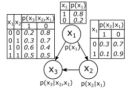
In a Bayesian network model, a directed acyclic graph (DAG) represents graphically the relation between random variables [17], [18]. Assume that the DAG is comprised of p random variables, denoted X={X1=x1,…, Xp=xp}. These variables are linked through edges to reflect dependencies between variables (see Figure 1).
[image:4.612.110.243.523.615.2]In BN terminology a node x1 is said to be a parent of another node x2 if there exists an edge from x1 to x2, and x2 is a child of x1.
Figure 1.Discrete Bayesian network example.
The directed edges in the DAG represent dependencies. Statistically, dependencies between random variables are quantified through conditional probabilities. For instance the conditional probability of node x2dependent on node x1, P(x2 | x1), is specified as follows (Figure 1):
(1)
)
(
/
)
(
)
|
(
x
2x
1P
x
2x
1P
x
1P
From the conditional probability in equation (1), Bayes’ theory states that the posterior probability, P(x2|x1), can be estimated by multiplying the likelihood, P(x1|x2), and the prior probability,
P(x2), and normalizing with the probability of evidence, P(x1):
(2)
)
(
/
)
(
)
|
(
)
|
(
x
2x
1P
x
1x
2P
x
2P
x
1P
Through the application of the Bayes’ theorem in equation (2)
inferences are performed in the Bayesian network model, i.e. updating the probabilities of nodes given new observations. To this end, the qualitative causal structure of the DAG is exploited systematically. However, prior to the inference task, the structure of the DAG and likelihood values have to be specified through expert knowledge or learning algorithms.
Bayesian networks are a compact representation of joint probability distributions [17]. In probability theory, the chain rule permits the calculation of any member of the joint distribution of a set of random variables using conditional probabilities [17]. Accordingly the joint distribution of the set of random variables
X={X1=x1,…, Xp=xp} is defined as follows:
(3) )
,..., | ( )
(
1
1 1
p
i
p
i x x
x P X
P
Using the information encoded in the DAG, equation (3) can be simplified to account only for parent nodes. Namely, if X is comprised of discrete random variables (e.g., Figure 1), the joint probability density function (the global distribution) is represented as a product of conditional probability distributions (the local distributions associated with each variable xi
X, 1<i<p) [17]:(4) ) | ( P (X)
1
pa(i)
p
i
i x
x P
where xpa(i) is the set of parents of xi and P(xi|xpa(i)) is the conditional probability distribution containing one distribution for each variable. If instead X is comprised of continuous random variables, the BN model is known as a Gaussian Bayesian network (GBN) model, and the joint probability density function is defined as [17]:
(5) ) | ( (X)
1
pa(i)
p
i
i x
x f P
where f denotes the conditional Gaussian probability density function containing one density function for each continuous random variable.
The strength of relations among dependent nodes are synthesized through conditional probability tables (CPT). CPTs are defined for each node xi
X of the BN model expressing the conditional probability distributions (CPD) for all the parent nodesxpa(i). If the nodes are discrete random variables, the CPD can be expressed as a multinomial distribution (see Subsection 6.1), and for continuous random variables, dependencies are expressed through Normal distributions (see Subsection 6.2) [17].
In the discrete case, if a node does not have parents (also known as a root node) it will have a marginal probability table (e.g., node
parent nodes (nodes x2 and x3 in Figure 1). In the continuous case, the CPT of the root nodes will be specified with a univariate Normal distribution. If the node has parents, the CPD will be a linear combination of Gaussian distributions.
A BN model is completely defined by the DAG and the conditional probabilities between the nodes, i.e. BN=(DAG, θ), where θ denotes the parameters of the CPT. The process of estimating the conditional probabilities between nodes is called parameter learning and the process of estimating the posterior distributions (i.e. diagnosis in the presence of specific data) is called probabilisticinference.
3.1 PARAMETER AND STRUCTURE LEARNING CPT values can be estimated via parameter estimation techniques both for continuous and discrete random variables. Classical examples of parameter learning techniques for Bayesian networks include maximum likelihood estimation (MLE) and Bayesian estimation [17]. This paper focuses on the MLE algorithm by maximizing the likelihood of making the observations given the parameters.
Given a training dataset D={D1,…,D|train|}, first it is necessary to estimate the likelihood L that the dataset was generated by the Bayesian network BN=(DAG , θ), and then to find the maximum likelihood estimator,
ˆ, as follows:(6) )} | ( max{ arg
ˆ L D
The MLE algorithm can be seen as the maximization of the agreement between the selected parameters and the observed data. Depending on the discrete or continuous nature of the random variables, the CPD will be modelled with different distributions and the likelihood will be different (see Subsections 6.1 and 6.2 for DGA examples).
It is also possible to learn from a dataset the structure of the DAG. The problem in this case focuses on finding a BN structure which maximizes the value of a scoring function. In order to deal with possible overfitting issues, different information criteria are used as scoring functions (e.g., Akaike or Bayesian information criterion [18]). The structure optimization problem can be solved through different metaheuristics, and this process is called structure learning [17]. The work below focuses on parameter learning steps and the DAG model is elicited from knowledge derived from DGA standards. Therefore, structure learning techniques are not considered further here.
3.2 PROBABILISTIC INFERENCE
After determining the structure of the Bayesian network and learning the parameters, the BN model can be used to make inferences. The goal of this work is to perform diagnosis or causal analysis: reasoning from effects (measured DGA values) to causes (transformer faults).
The causal analysis consists of updating the probabilities of unobserved nodes through the BN and making inferences about the most probable status of the system. That is, measured gas values are given as evidence to the BN model and through the DAG structure the posterior probability of possible causes is
evaluated, P(transformer fault | gas data).
The posterior probability of each node enables inferences to be made about the status of unobserved parameters and the most likely status for the node. The inference process is different for discrete and continuous cases (see Subsections 6.1 and 6.2 for details).
4 I
NTRODUCTION TOIEC
TC10
D
ATASET The IEC TC 10 [9] dataset contains sets of seven different gases: ethane (C2H6), ethylene (C2H4), hydrogen (H2), methane(CH4), acetylene (C2H2), carbon monoxide (CO), and carbon
dioxide (CO2) sampled from different transformers, and
labelled with their corresponding fault mode. Faults are classified into Normal degradation samples, Thermal faults (T<700°C and T>700°C), Arc faults (low and high energy discharges), and partial discharge (PD) faults.
In order to generate this database, faulty equipment was removed from service, visually inspected by experienced engineers and maintenance experts, and the fault clearly identified. In all cases relevant DGA results were available [9]. The IEC TC 10 database also contains typical normal degradation values observed in several tens of thousands of transformers operating on more than 15 individual networks.
In total, the dataset is comprised of 167 samples but it is not well balanced in relation to proportions of classification types, e.g. 5.3% partial discharge failure samples, 44.4% arcing failure samples, 20.4% thermal failure samples and 29.9% normal degradation samples. The classification of unbalanced datasets becomes challenging, especially for those classes which have a smaller proportion of data samples, i.e. partial discharge in this case. One direct solution is to balance the dataset by resampling the data samples for the classes that have fewer data samples and change the classification problem into a balanced classification problem. However, this may also have consequences for generalization and adoption in industry (see Section 2). Therefore, this work focuses on unbalanced classification problems without modifying the data.
5 N
ORMALITYT
ESTING OFIEC
TC
10
D
ATASET Since Bayesian networks with continuous variables use Normal distributions for learning and inference tasks, the data that bestfit with this distribution is expected to generate the most useful information for diagnosis. Accordingly, a hypothesis test is implemented to analyze if the gases in the IEC TC 10 dataset come from the Normal distribution. The following hypotheses are defined: H0=data is consistent with the Normal distribution
H1=data is not consistent with the Normal distribution
There are different tests to evaluate the Normality of the data and verify if the null hypothesis is satisfied [19]. The main difference among different tests is on the evaluated Gaussian properties. Test values represent the error when approximating with a Normal distribution and therefore the lower the test values, the greater the confidence in the null-hypothesis. For simplicity this paper focuses on two different tests.
[19]. The JB test measure is given by:
K-3
(7) 24n S
6
2 2
n
JB
where n is the number of samples, S is sample skewness, and K is kurtosis.
On the other hand, the Cramer-von Mises (CvM) testevaluates the approximation error based on the empirical cumulative distribution function [19]:
1/12
n
/
2 1
/2
(8)1 i
2
n x i n
CvM i
where Φ is the cumulative distribution function of the Normal distribution, µ and σ are the mean and standard deviation of data values, and n is the number of samples.
In order to evaluate the representativeness of the results, p-values are also calculated. The p-values are defined as the probability of obtaining a result equal to or more extreme than was actually observed, when the null hypothesis is true. The greater the p-value, the higher the confidence (weight) in the null-hypothesis (i.e., data comes from a Normal distribution). A widely accepted criterion is that if the p-value is below 0.05 the null hypothesis can be rejected (i.e. 95% of the times the null hypothesis H0 will be
[image:6.612.312.568.131.406.2]correctly rejected), otherwise it is considered to be valid. Table 2 displays the results obtained from the Normality tests.
Table 2.Normality test results.
Test Jarque-Bera Cramer - von Mises
Score p Score p
C2H6 0.34 0.83 0.077 0.22
C2H4 0.69 0.67 0.14 0.02
H2 1.36 0.44 0.12 0.05
CH4 2.74 0.18 0.08 0.15
C2H2 4.5 0.08 0.17 0.01
CO 25.69 0.003 0.83 8e-9 CO2 43.3 0.001 0.83 8e-9
It is possible to see in Table 2 that both tests suggest that the best fitted gas is C2H6, and the worst fitted gases are C2H2, CO
and CO2. Differences between both tests when ranking the rest
of the gases (C2H4, H2, CH4) arise from the underlying
properties of each test, however, their p-values suggest consistently that the null hypothesis can be accepted. The score and p-values of CO and CO2 gases suggest that the null
hypothesis cannot be accepted, and therefore, it cannot be assumed that these gases follow a Normal distribution.
6 B
AYESIAND
IAGNOSISF
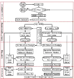
RAMEWORKFigure 2 shows the proposed Bayesian diagnosis framework divided into four main phases: cross-validation, data preprocessing, learning and inference. The left path through the chart is dedicated to discrete random variables and the process in the right path is suited for continuous random variables.
The goal of the cross-validation stage is to (i) validate each of the generated BN models by obtaining more accurate estimates of the classification performance of the proposed framework, and (ii) assess how the diagnostics results will generalize to an independent dataset. To this end, Monte Carlo cross-validations are implemented through the following steps [20]:
(1) Initialize the trial counter, trials=0;
(2) Random shuffle the dataset and execute preprocessing, learning and inference steps, and store the results;
(3) If trials<Max_trials, iterate from the previous step and increase the trial counter by 1;
(4) If trials=Max_trials, end the loop, and then extract mean and standard deviation of the stored diagnosis results;
Figure 2.Proposed Bayesian framework.
For each trial, the random shuffle and the train/test steps generate different training and testing datasets, and therefore, this process trains and tests the framework with Max_trials different training and testing datasets (Max_trials=103 trials in this paper).
As a results this validation process enables higher confidence and consistency in the diagnosis results [20].
The data preprocessing stage starts by applying a log-scale step. This step is applied because diagnostic information does not reside in absolute gas values but instead in the order of magnitude [10]. Firstly, the logarithm of every gas sample in the dataset is taken and then each variable in the dataset is scaled to mean zero and standard deviation one. This is done for each gas within the dataset, by subtracting the mean value and dividing by the standard deviation, for each sample of the variable.
Subsequently, different preprocessing, learning and inference algorithms are implemented depending on the nature of the DGA data. In both discrete and continuous configurations, as shown in Figure 2, the dataset is divided into train/test datasets using the 80% and 20% of the randomly shuffled dataset, respectively. The different activities for discrete and continuous datasets are explained in Subsections 6.1 and 6.2 below.
[image:6.612.90.256.357.454.2]transformer insulation failure modes into: Thermal, Arc, PD
(partial discharge), and Normal degradation. This classification is also in agreement with the IEC TC 10 case study dataset, which includes samples for each of these failure fault modes.
The R bnlearn package [18] was used for the implementation of learning and inference tasks of the discrete and continuous Bayesian network models reported here.
6.1 PROBABILISTIC DGA THROUGH DISCRETE BAYESIAN NETWORKS
In a discrete Bayesian network model, the conditional probability distributions with discrete random variables, P(xi|xpa(i)), are commonly expressed through multinomial distributions [17].
If an experiment which can have k outcomes is performed n
times and xi denotes the number of times the ith outcome is obtained, the mass function of the experiment (and the multinomial distribution) is defined as:
) 9 ( 0
,..., )
,..., , ; ,...,
( 1
1 1
1 1
otherwise n x if p x x
n p
p n x x f
k i i K
i x i k k
k
i
In this work n will correspond to the number of training gas samples, and k will be the possible set of discretized outcomes of the sample. The discretization process is explained below.
The key data preprocessing step for discrete BN models is the discretization process. Using the intervals defined by the ratio-based techniques (Doernenburg, Duval, Rogers), all the DGA data can be discretized according to each ratio-based technique.
Table 3 shows the original Doernenburg’s classification ratio values, where R1=CH4/H2, R2=C2H2/C2H4, R3=C2H2/CH4 and
[image:7.612.355.534.148.229.2]R4=C2H6/C2H2 [5].
Table 3.Original Doernenburg’s classification ratios [5]. R1 R2 R3 R4 Diagnosis
>1 <0.75 <0.3 >0.4 Thermal <0.1 N/A <0.3 >0.4 PD 0.1-1 >0.75 >0.3 <0.4 Arcing
[image:7.612.83.264.459.511.2]The classification intervals in Table 3 were discretized through the coding shown in Table 4, where the ranges for each ratio were drawn from [5].
Table 4.Doernenburg’s coding values.
Ratio R1 R2 R3 R4
Code 0 1 2 0 1 0 1 0 1
Range ≤0.1 0.1-1 >1 ≤0.75 >0.75 ≤0.3 >0.3 ≤0.4 >0.4
This way it is possible to transform any absolute gas values into discretized Doernenburg’s code values.
The coding for the occurrence of failure modes is specified with binary coding (1: occurred, 0: non-occurred), e.g. PD=0, Arc=0,
Thermal=1, and Normal=0 denotes a thermal fault.
The same codification process was applied for the Duval’s triangle and Rogers’ ratio techniques (see Appendix).
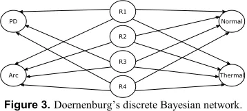
In order to design the BN structure the links between ratios and fault types were examined. For instance, Figure 3 shows the discrete BN model for the Doernenburg´s ratio technique, where
Thermal and Arc faults are determined using R1, R2, R3 and R4;
and PD uses R1, R3 and R4. Although the classification ratios in
Table 3 do not include normal degradation values, when designing the BN model it is assumed that the Normal condition is indicated by the remainder values of all the ratios (i.e. when there is no diagnosis of Thermal, Arc, or PD). This allows the model to be trained for normal data.
Figure 3.Doernenburg’s discrete Bayesian network.
After designing the BN structure, it is possible to estimate the conditional probability tables corresponding to each node through the maximum likelihood estimation algorithm. In order to simplify the maximization process the logarithm of the likelihood function was used, i.e. log-likelihood, LL. The log-likelihood of the training dataset D = {D1,…, D|train|} is:
| ,
(10)log
n
1 i
| |
1
) (
train k
k i pa
i x D
x P LL
It is possible to see that the scoring function in equation (10) decomposes into a series of terms, one per node xi. The next step is the estimation of the parameters of each node’s conditional probability values given its local training data. Using the multinomial distribution defined in equation (9) the closed form solutions for the log-likelihood function can be obtained (see [17] for more details).
The outcome of the learning step is the set of conditional probability tables which specify the conditional probabilities for each node. Table 5 shows the CPT for a specific configuration of the Doernenburg BN model.
Table 5.Subset of theconditional probability table learned from data. R1 PD=0, Arc=0, Thermal=1, Normal=0
0 0.04
1 0.08
2 0.88
From the example in Table 5 one can deduce that when there is a Thermal fault, the value of R1 is very likely (88%) to be in the
range determined by the discretized number 2 (R1>1, see Table 4).
Tracing back this value to the original Doernenburg’s ratio (see Table 3) it is possible to see that this matches with a Thermal fault. This example node supplies one piece of probabilistic evidence for diagnosis. By utilizing the evidence from all nodes for a given sample, one can evaluate probabilistically all the possible failure types. It is possible to see the benefit of using a probabilistic diagnosis framework, where instead of giving a single output, more information about the strength of belief in a given diagnosis is combined into the overall decision.
The next step is the inference step (Figure 2). To this end, the conditional probability queries are implemented (i.e.,
[image:7.612.44.303.570.611.2]which combines rejection sampling and uniform weights [17]. The main idea is to generate a set of random variables and then estimate the posterior probability, P(xi|xpa(i)), taking as input the Bayesian network with N nodes X={X1, …, XN}, and the evidence
(or test) data E={e1,…,e|test|}. For instance, P(PD=1|e1) is inferred given the BN in Figure 3 and e1={R1=1, R2=1, R3=1} as follows:
(1) Initialize counters: evidence, count(e)=0, and joint scenario and evidence, count(x, e)=0;
(2) Prior distribution sampling specified by the BN: generate random samples from parents to children in the BN model in topological order. Once parents are sampled proceed in the BN structure to obtain the conditional probabilities of children. Discretize the results;
(3) If the generated samples do not satisfy evidence reject them, otherwise if they satisfy the evidence (i.e. R1=1,
R2=1 and R3=1) then increase count(e) by 1;
(4) If both the scenario and the evidence are true (i.e. PD=1, R1=1, R2=1 and R3=1), then increase count (x, e) by 1;
(5) Repeat steps (2)-(4) for a large number of times;
(6) Estimate the posterior, P(x|e), as follows:
P(x|e)=count(x, e)/count (e).
Given the test data with discretized ratio values and the Bayesian network model, this algorithm infers the probability of each failure mode. The failure mode with the highest likelihood is the final diagnosis of the model.
The same data processing, learning and inference steps are applied for the Duval and Rogers based diagnosis techniques (see Appendix).
6.2 PROBABILISTIC DGA THROUGH GAUSSIAN BAYESIAN NETWORKS
Ratio techniques lend themselves well to discrete Bayesian networks, since the ratios are analyzed based on discrete ranges specified by each technique. However, these ranges present crisp decision boundaries. It may be expected that DGA samples close to a ratio boundary will have a different likelihood of indicating a fault than another sample near the middle of the range. One method of capturing this variation is to treat the ratios as continuous random variables.
When a Bayesian network is comprised of continuous random variables the probability tables are replaced by continuous distributions. A widely implemented approach adopted in this paper is the use of Gaussian Bayesian networks (GBN) [17], [18]. In a GBN the conditional probability distributions are defined through linear Gaussian distributions and local distributions are modelled through Normal random variables, whose density function is defined as:
x-
(11) 21 -exp 2 1 )
, | (x
2
2
f
where x is the variable under study, µ is the mean and σ2 is the variance, often denoted as x~N(µ, σ2).
Local distributions are linked through linear models in which the parents play the role of explanatory variables. Each node xi is regressed over its parent nodes. Assuming that the parents of xi are
{u1,…,uk}, then the conditional probability can be expressed as
p(xi|u1,…,uk) ~ N(β0 + β1u1+ …+ βkuk; σ2), that is:
... (12)
2 1 -exp 2 1 ) ,..., | (
2 1
1 0
1
k k
k i
u u
x u
u x p
[image:8.612.329.539.129.258.2]where β0 is the intercept and {β1,…, βk} are the linear regression coefficients for the parent nodes {u1,…,uk}.
Figure 4 shows the DAG for the GBN model with all gases. It is assumed that all gases affect each of the failure modes.
Figure 4.GBN model for all gases configuration.
As in the discrete BN case, the parameter learning process is implemented through maximum likelihood estimation by using the MLE expression derived from the linear Gaussian density function [17]. The log-likelihood of the training dataset
D = {D1,…, D|train|} is a sum of terms for each node i:
| ,
(13)log
n
1 i
| |
1 ()
train
k i pai k
D x
x f LL
Using the linear Gaussian distribution to define the conditional probability values, f(xi|xpa(i)), the closed-form solution of log-likelihood can be estimated (see [17] for more details).
The outcome of the learning step is the set of conditional probability tables which specify the conditional probability density functions for each node. Focusing on the GBN model shown in Figure 4, the model is first trained with the training set, i.e. a matrix with 8 columns (7 gas values and the failure mode) and 134 rows. The learning step estimates the corresponding parameters for each node in the BN model, e.g. for the Arc
node: P(Arc | C2H6, C2H2, CH4, C2H4, CO2, CO, H2) ~ N(β0 +
β1C2H6 + β2C2H2 + β3CH4 + β4C2H4 + β5CO2 + β6CO + β7H2; σ2).
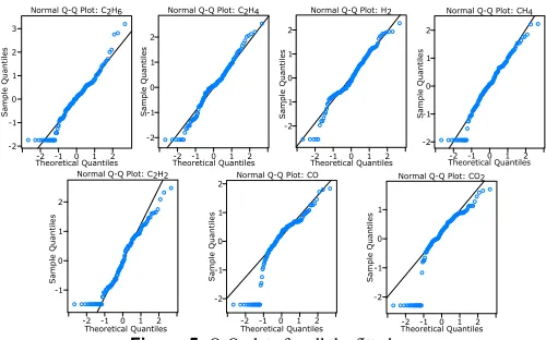
[image:8.612.314.564.571.727.2]As the graphical representation of the fitted distribution becomes complex with more than two parent nodes, the goodness-of-fit of the distributions for each gas node are examined. Figure 5 shows the Q-Q plots based on the quantiles of the fitted Normal distributions.
Figure 5 confirms the Normality test results displayed in Table 2, that is, CO and CO2 do not follow the Normal distribution. Therefore, a second GBN was trained with the dataset of only Normally distributed gases.
Probabilistic inference for a GBN is based on the likelihood weighting (LW) algorithm [17]. Likelihood weighting is a form of importance sampling which fixes the test DGA gas samples (evidence) and uses the likelihood of the evidence to weight samples. The LW algorithm calculates the weighted probability of occurrence of a given node Xi
X, where X={X1,…,Xn}; given the evidence E={e1,…,e|test|}. For example, P(PD|e1) is inferred given the BN in Figure 4, with Xi=PD and e1={C2H6=0.5, C2H2=0.8,CH4=0.1, C2H4=0.81, CO2=0.25, CO=0.05, H2=0.1} as follows:
(1) Initialize W, a vector of weighted counts for each possible value of PD
(2) For each variable Xi X, where X={X1,…Xn} (Figure 4)
a. Initialize wi=1
b. If Xi is an evidence variable with value xi in E, e.g. C2H6=0.5:
i. assign Xi=ei;
ii. compute wi=wi.P(ei|xpa(i))
c. If Xi is not an evidence variable
i. draw a random sample xi~P(Xi|xpa(i))
(3) Update the weight vector, W[Xi]=W[Xi]+wi
(4) Repeat previous steps (2)-(3) for K samples to be generated (also known as particles);
(5) Normalize the weight vector
When applied to the DGA dataset, for each of the analyzed failure modes, fi, the outcome of the inference is a set of weighted values (i.e., the pair [wi, xi]; with 1<i<K), whose density values
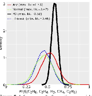
[image:9.612.96.253.460.624.2]can be calculated through Kernel density estimates [21]. Figure 6 shows an inference outcome example of a GBN model trained and tested with Normally distributed gases.
Figure 6.Inference results for continuous variables.
In order to determine the cause of the fault, the maximum likelihood values among the failure modes are compared. The x-axis in Figure 6 denotes random samples drawn from the conditional distribution of the node given the evidence, Pr(fi|C2H6,C2H4, H2, CH4, C2H2). The x-axis value of the peak
density indicates the maximum likelihood value. That is, the PD fault is the likely cause of failure.
Inference results enable informed decision-making taking
into account the uncertainty criteria. This information becomes critical for engineers when they have different methods and they need to reach a conclusion about the cause of the fault. That is, different maintenance decisions can be studied not only from the perspective of the highest likelihood value, but also considering distribution function. For instance, the narrower the width of the density function, the higher the confidence of the GBN model in its final diagnosis. This information is lost with most of the AI methods because their classification results are either a binary value or a deterministic probability value and therefore, the uncertainty cannot be accurately captured for subsequent maintenance decisions.
7 R
ESULTSFirstly the results obtained from the application of the traditional ratio-based techniques are analyzed, without applying Bayesian networks, defined in Table 3 (Doernenburg), Table 9 (Duval) and Table 11 (Rogers). Table 6 displays the obtained accuracy results after performing 103 trials and extracting mean and standard
deviation from all the gathered accuracy results. This process is applied to the overall accuracy and to the accuracy for the diagnosis of each specific failure mode.
From Table 6 it is possible to see that Doernenburg and Duval methods do not diagnose normal degradation transformers and this impacts negatively on the overall classification accuracy. However, note that these techniques are very good at identifying partial discharge faults (Duval) and arcing faults (Duval, Doernenburg).
Table 6.Ratio-based diagnosis results.
Approach Overall Thermal Accuracy PD Arc Normal
Rogers 42.39% ± 7.4% 58.5% ± 18.72% 12.7% ± 33.53% 66.2% ± 11.4% 3.7% ± 11%
Doern. 60.8% ± 6.5% 74.3% ± 16.9% 73.9% ± 35.2% 94% ± 6% 0%
Duval 68.9% ± 7.2% 87.7% ± 12.6% 96.9% ± 17% 100% 0%
Table 7 displays the results obtained by applying the Bayesian framework for the analyzed cases. Discrete Bayesian network models improve the diagnosis accuracy with respect to the ratio-based diagnosis techniques displayed in Table 6.
Table 7.Bayesian network results.
Approach Overall Thermal Accuracy PD Arc Normal
Rogers 73.76% ± 7.2% 70.2% ± 18% ± 13.6% 34.08% 93.72% ± 6.1% 61.5% ± 15.8%
Doern* 79.86% ± 6.6% 74.3% ± 16.9% 73.9% ± 35.2% 94% ± 6% 64% ± 15%
Duval* 72.8% ± 7% 49.9% ± 20.2% 96.3% ± 18.8% 96.3% ± 5% 49.7% ± 16.1%
GBN: All gases
80.9% ± 6.6%
67.7% ± 18.5%
81.1% ± 11.3%
93.94% ± 6.5%
73.07% ± 14.9% GBN:
Normal gases
82.3% ± 6.6%
68.7% ± 17.4%
94.4% ± 6.8%
94.19% ± 6.8%
72.9% ± 15.4%
* including normal states in the BN model
degradation. However, the Rogers BN also shows an overall improvement. Note that the Normal degradation state has been taken into account by assuming that all the gas ratios may generate this state (see Figures 3, 7, and 8 for Doernenburg, Duval and Roger discrete BN models). The GBN models give further improvement. Among the GBN models, inclusion of only Normally distributed gas variables gives best results with a maximum overall accuracy of 88.9%, i.e. 82.3%+6.6%.
Note that Table 7 reports mean accuracy and standard deviation values and avoids reporting only absolute maximum accuracy results because this can lead to over-optimistic conclusions. All the models in Table 7 have been examined 103 times in order to validate and generalize the results
according to the Monte Carlo cross-validation method (see Figure 2). For each trial, firstly the dataset is randomly shuffled, then it is divided into training and testing datasets and finally, learning and inference steps are completed. In total, the models in Table 7 are trained 103 times and tested for
33103 data samples.
Focusing on the accuracy of the Bayesian network models for specific failure modes, note that the Thermal fault is best captured by Doernenburg’s ratio values (mean accuracy 74.3%); the PD fault is best captured with Duval’s gas values (mean accuracy 96.3%); the Arc fault is best captured by the GBN based on Normally distributed gas variables (mean accuracy 94.19%), and finally the Normal degradation is best modelled with the GBN model with all gas variables (mean accuracy 73.07%). Note also that due to the underlying assumptions of the inference algorithms at times it is possible to have variance bounds exceeding the accuracy limits, e.g. Duval’s PD fault in the discrete BN model.
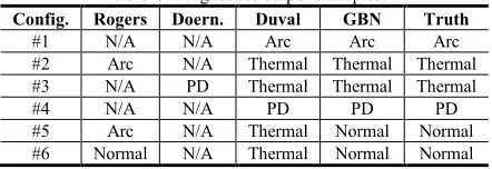
[image:10.612.63.284.568.644.2]Although the number of samples for the PD fault is small compared with the rest of classes (Section 4), Table 7 shows that the continuous BN model effectively learns the conditional distribution of this fault. This happens because the trend of the PD samples in the dataset is predictable (as confirmed by the Duval’s triangle results in Table 6) and the pattern can be described with few samples. The Arc degradation samples are accurately predicted by the Duval triangle too, but if Normal degradation samples were considered, there will be an increased number of false positives (see Table 8).
Table 8.Diagnostics output examples.
Config. Rogers Doern. Duval GBN Truth
#1 N/A N/A Arc Arc Arc
#2 Arc N/A Thermal Thermal Thermal #3 N/A PD Thermal Thermal Thermal
#4 N/A N/A PD PD PD
#5 Arc N/A Thermal Normal Normal #6 Normal N/A Thermal Normal Normal
Table 8 displays some DGA samples covering all conditions, the observed truth health state, and the outcome of the best GBN configuration in Table 7 along with the outcome of classical DGA methods. These are the gas values for each configuration (all units in ppm):
#1 H2=1330, CH4=10, C2H2=182, C2H4=66, C2H6=20.
#2 H2=66, CH4=60, C2H2=1, C2H4=7, C2H6=2.
#3 H2=2031, CH4=149, C2H2 =1, C2H4=3, C2H6=20.
#4 H2=9340, CH4=995, C2H2 =7, C2H4=6, C2H6=60.
#5 H2=200, CH4=50, C2H2=30, C2H4=200, C2H6=50.
#6 H2=134, CH4=134, C2H2=1, C2H4=45, C2H6=157.
Figure 6 shows the classification result of the configuration #4 inferred from the proposed GBN model.
8 C
ONCLUSIONDGA is a mature and industry-standard method that focuses on the measurement of dissolved gasses over time. Classical DGA methods (Duval’s triangle, Roger’s ratios, Doernenburg’s ratios) use crisp decision bounds, they assign 100% belief to a single failure mode, and they classify different failure modes. Different black-box artificial intelligence models have been proposed so as to improve the accuracy of the classical DGA methods. However, the diagnostics outcome of the proposed models is a deterministic probability value and they lack an explanation of physical significance because they represent the correlation obtained from the training data. This may represent challenges to interpret conflicting results, post-process the results, and adopt informed decisions.
In this context, this paper presents a novel method for transformer diagnosis based on Gaussian Bayesian networks (GBNs). This method not only transforms crisp decision bounds into probability functions, but also the inference of the likelihood of each failure mode reflects the uncertainty associated with the decision-making process, and it enables the integration of expert knowledge and data through a causal representation of causes and consequences. Distribution functions and causal relationships become crucial from a practical end-use perspective. That is, when different methods classify different faults, maintenance decisions can be studied from the perspective of the inferred density functions for an informed decision-making under uncertainty.
The results obtained in this paper can be used as a benchmark to other techniques because the IEC TC 10 dataset is publicly available [9]. So as to make consistent and fair comparisons, it is necessary to implement classifiers modelled and tested in the same conditions. The model presented in this paper was validated using Monte Carlo cross-validation which enables the extraction of general accuracy statistics. Besides, this work was focused on a multiclass classification problem classifying normal, partial discharge, thermal and arcing samples. In these conditions the maximum accuracy of the proposed GBN model is of 88.9%.
This paper also highlights the importance of using data distributions well-fitted with the diagnostics model. Although some methods have been extended for generic distributions, some techniques such as GBNs are limited to the application of a given distribution function, and in this situation hypothesis testing becomes a critical tool for selecting an appropriate technique. In this case the Normality of the data was tested using various methods and accordingly the best fitted gas values were selected.
in order to incorporate all available gases.
APPENDIX
The original classification scheme for Duval’s triangle proposed in [8] evaluates the relative amount of three gasses (C2H2, CH4, C2H4) and classifies them within the coordinates of a
[image:11.612.323.553.101.144.2]triangle. Fault regions within the triangle can be transformed into a numerical classification method as displayed in Table 9 [22].
Table 9.Duval’s classification ratios [22]. C2H2% CH4% C2H4% Diagnosis
0-0.02 0.98-1 0-0.02 PD
0-0.04 0.76-0.98 0.46-0.8 0.02-0.2 0.2-0.5 Thermal 300°C<T<700°C Thermal T<300°C
0-0.15 0-0.5 0.5-1 Thermal T>700°C 0.04-0.13 0.47-0.96 0-0.4
Mixture of thermal and electrical faults 0.13-0.29 0.21-0.56 0.4-0.5
0.15-0.29 0-0.35 0.5-0.85 0.13-0.29 0.31-0.64 0.23-0.4
High energy discharge 0.29-0.77 0-0.48 0.23-0.71
0.13-1 0-0.87 0-0.23 Low energy discharge
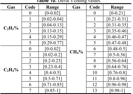
[image:11.612.48.299.170.290.2]The classification intervals in Table 9 can be discretized through the coding shown in Table 10.
Table 10.Duval’s coding values.
Gas Code Range Gas Code Range
C2H2%
0 [0-0.02]
CH4%
0 [0-0.21] 1 [0.02-0.04] 1 [0.21-0.31] 2 [0.04-0.13] 2 [0.31-0.35] 3 [0.13-0.15] 3 [0.35-0.46] 4 [0.15-0.29] 4 [0.46-0.47] 5 [0.29-0.77] 5 [0.47-0.48]
C2H4%
[image:11.612.61.287.329.488.2]0 [0-0.02] 6 [0.48-0.5] 1 [0.02-0.2] 7 [0.5-0.56] 2 [0.2-0.23] 8 [0.56-0.64] 3 [0.23-0.4] 9 [0.64-0.76] 4 [0.4-0.5] 10 [0.76-0.8] 5 [0.5-0.71] 11 [0.8-0.96] 6 [0.71-0.85] 12 [0.96-0.98] 7 [0.85-1] 13 [0.98-1]
[image:11.612.101.256.529.581.2]Figure 7 shows the Bayesian network model corresponding to Duval’s triangle.
Figure 7.Duval’s discrete Bayesian network.
Rogers’ ratios (R1=CH4/H2, R2=C2H2/C2H4, R5=C2H4/C2H6)
were proposed in [7]. Table 11 displays the coding scheme used by the Rogers’ ratio method.
Table 11.Original Rogers’ classification ratios [7].
R1 R2 R5 Diagnosis
>0.1-1 <0.1 <1 Normal degradation <0.1 <0.1 <1 PD 0.1-1 0.1-3 >3 Arcing >0.1-1 <0.1 1-3 Low temperature thermal
>1 <0.1 1-3 Thermal <700°C >1 <0.1 >3 Thermal >700°C
The classification intervals in Table 10 can be discretized through the coding shown in Table 12.
Table 12.Rogers’ coding values.
Ratio R1 R2 R5
Code 0 1 2 0 1 2 0 1 2
Range ≤0.1 0.1-1 >1 ≤0.1 1-3 >3 ≤1 1-3 >3
Figure 8 shows the BN model corresponding to the Rogers’ ratio model.
Figure 8.Rogers’ discrete Bayesian network.
REFERENCES
[1] V. M. Catterson, S. D. J. McArthur, and G. Moss, "Online Conditional Anomaly Detection in Multivariate Data for Transformer Monitoring," IEEE Trans. Pow. Del., vol. 25, pp. 2556-2564, 2010.
[2] V. M. Catterson, J. Melone, and M. S. Garcia, "Prognostics of transformer paper insulation using statistical particle filtering of on-line data," IEEE Electr. Insul. Mag., vol. 32, pp. 28-33, 2016.
[3] "IEEE Guide for the Evaluation and Reconditioning of Liquid Immersed Power Transformers," IEEE Std C57.140-2006, pp. c1-67, 2007. [4] J. I. Aizpurua and V. M. Catterson, "ADEPS: A Methodology for
Designing Prognostic Applications," in Proceedings of the Third European Conf. of the PHM Society 2016, Bilbao, Spain, 2016, p. 14. [5] "IEEE Guide for the Interpretation of Gases Generated in Oil-Immersed
Transformers," IEEE Std C57.104-2008 (Revision of IEEE Std C57.104-1991), pp. 1-36, 2009.
[6] A. Abu-Siada and S. Islam, "A new approach to identify power transformer criticality and asset management decision based on dissolved gas-in-oil analysis," IEEE Trans. Dielectr. Electr. Insul., vol. 19, pp. 1007-1012, 2012.
[7] R. R. Rogers, "IEEE and IEC Codes to Interpret Incipient Faults in Transformers, Using Gas in Oil Analysis," IEEE Trans. Dielectr. Electr. Insul., vol. EI-13, pp. 349-354, 1978.
[8] M. Duval, "A review of faults detectable by gas-in-oil analysis in transformers," IEEE Electr. Insul. Mag., vol. 18, pp. 8-17, 2002. [9] M. Duval and A. dePablo, "Interpretation of gas-in-oil analysis using
new IEC publication 60599 and IEC TC 10 databases," IEEE Electr. Insul. Mag., vol. 17, pp. 31-41, 2001.
[10] P. Mirowski and Y. LeCun, "Statistical Machine Learning and Dissolved Gas Analysis: A Review," IEEE Trans. Power Del., vol. 27, pp. 1791-1799, 2012.
[11] W. H. Tang, Z. Lu, and Q. H. Wu, "A Bayesian network approach to power system asset management for transformer dissolved gas analysis," in Int. Conf. on Electric Utility Deregulation and Restructuring and Power Technologies, 2008, pp. 1460-1466.
[12] L. Wang, X. Zhao, J. Pei, and G. Tang, "Transformer fault diagnosis using continuous sparse autoencoder," SpringerPlus, vol. 5, p. 448, 2016.
[13] A. Abu-Siada, S. Hmood, and S. Islam, "A new fuzzy logic approach for consistent interpretation of dissolved gas-in-oil analysis," IEEE Trans. on Dielectr. Electr. Insul., vol. 20, pp. 2343-2349, 2013.
[14] A. Shintemirov, W. Tang, and Q. H. Wu, "Power Transformer Fault Classification Based on Dissolved Gas Analysis by Implementing Bootstrap and Genetic Programming," IEEE Trans. Syst., Man, Cybern. C, vol. 39, pp. 69-79, 2009.
[16] Y. Sun, M. S. Kamel, A. K. C. Wong, and Y. Wang, "Cost-sensitive boosting for classification of imbalanced data," Pattern Recognition, vol. 40, pp. 3358-3378, 2007.
[17] R. E. Neapolitan, Learning bayesian networks: Prentice Hall, 2004. [18] R. Nagarajan, M. Scutari, and S. Lbre, Bayesian Networks in R: with
Applications in Systems Biology: Springer Publishing Company, Incorporated, 2013.
[19] T. Thadewald and H. Büning, "Jarque–Bera Test and its Competitors for Testing Normality – A Power Comparison," Journal of Applied Statistics, vol. 34, pp. 87-105, 2007/01/01 2007.
[20] Q.-S. Xu and Y.-Z. Liang, "Monte Carlo cross validation," Chemometrics and Intelligent Laboratory Systems, vol. 56, pp. 1-11, 2001.
[21] K. JooSeuk and C. Scott, "Robust kernel density estimation," in IEEE Int. Conf. on Acoustics, Speech and Signal Processing, 2008, pp. 3381-3384.
[22] S. S. Desouky, A. E. Kalas, R. A. A. El-Aal, and A. M. M. Hassan, "Modification of Duval triangle for diagnostic transformer fault through a procedure of dissolved gases analysis," in IEEE Int. Conf. on Environment and Electrical Engineering, 2016, pp. 1-5.
J. I. Aizpurua (M’17) is a Research Associate within the Institute for Energy and Environment at the University of Strathclyde, Scotland, UK. He received the Eng., M.Sc. and the Ph.D. degrees from the Mondragon University (Basque Country, Spain) in 2010, 2012, and 2015 respectively. He was a visiting researcher in the Dependable Systems Research Group at the University of Hull (UK) during autumn 2014. His research interests include prognostics and health management, reliability, availability, maintenance and safety (RAMS) analysis and systems engineering for power engineering applications.
V. M. Catterson (M’06-SM’12) is a Senior Lecturer within the Institute for Energy and Environment at the University of Strathclyde, Scotland, UK. She received her B.Eng. (Hons) and Ph.D. degrees from the University of Strathclyde in 2003 and 2007 respectively. Her research interests include condition monitoring, diagnostics, and prognostics for power engineering applications.
Brian G Stewart (M’08) is Professor within the Institute of Energy and Environment at the University of Strathclyde, Glasgow, Scotland. He graduated with a BSc (Hons) and PhD from the University of Glasgow in 1981 and 1985 respectively. He also graduated with a BD (Hons) in 1994 from the University of Aberdeen, Scotland. His research interest are focused on high voltage engineering, electrical condition monitoring, insulation diagnostics and communication systems. He is currently an AdCom Member within the IEEE Dielectrics and Electrical Insulation Society.
Stephen D. J. McArthur (M’93–SM’07-F’15) received the B.Eng. (Hons.) and Ph.D. degrees from the University of Strathclyde, Glasgow, U.K., in 1992 and 1996, respectively. He is a Professor and co-Director of the Institute for Energy and Environment at the University of Strathclyde. His research interests include intelligent system applications in power engineering, covering condition monitoring, diagnostics and prognostics, active network management and wider smart grid applications.
B. D. Lambert is a Design Engineering Manager within Bruce Power. He received his B.Eng. degree from Lakehead University, Thunder Bay, Canada in 2012 and his P.Eng. from the Professional Engineers of Ontario in 2015. His design interests include large power transformers, high voltage transmission systems, as well as dielectric and insulating materials.
B. Ampofo is a Senior Technical Specialist within Bruce Power. He obtained his B.Eng. degree from Carleton University, Ottawa, Canada in 2006 and his P.Eng. from the Professional Engineers of Ontario in 2012. His design interests include large power transformers, high voltage transmission systems, as well as dielectric and insulating materials.
Gavin Pereira, a physical chemist, is currently a group leader of Kinectrics Inc.’s Petroleum Products research and testing group. He conducted his post-doctoral fellowship in ion-beam physics and Ph.D. in physical chemistry from the department of chemistry at the University of Western Ontario in London, Ontario. He finished his undergraduate degree at York University in Toronto, Ontario. His current role focuses on applied R & D and testing in additive chemistry, insulating oils, lubricating oils and greases.