Bivariate copula additive models for location, scale and shape

City, University of London Institutional Repository

Citation

: Marra, G. and Radice, R. ORCID: 0000-0002-6316-3961 (2017). Bivariate

This is the accepted version of the paper.

This version of the publication may differ from the final published

version.

Permanent repository link:

Link to published version

: http://dx.doi.org/10.1016/j.csda.2017.03.004

Copyright and reuse:

City Research Online aims to make research

outputs of City, University of London available to a wider audience.

Copyright and Moral Rights remain with the author(s) and/or copyright

holders. URLs from City Research Online may be freely distributed and

linked to.

City Research Online: http://openaccess.city.ac.uk/ [email protected]

Bivariate Copula Additive Models for Location, Scale

and Shape

Giampiero Marra

Rosalba Radice

Wednesday 15

February, 2017

Abstract

In generalized additive models for location, scale and shape (GAMLSS), the response

dis-tribution is not restricted to belong to the exponential family and all the model’s parameters

can be made dependent on additive predictors that allow for several types of covariate effects

(such as linear, non-linear, random and spatial effects). In many empirical situations,

how-ever, modeling simultaneously two or more responses conditional on some covariates can be

of considerable relevance. The scope of GAMLSS is extended by introducing bivariate

cop-ula models with continuous margins for the GAMLSS class. The proposed computational

tool permits the copula dependence and marginal distribution parameters to be estimated

si-multaneously, and each parameter to be modeled using an additive predictor. Simultaneous

parameter estimation is achieved within a penalized likelihood framework using a trust region

algorithm with integrated automatic multiple smoothing parameter selection. The introduced

approach allows for straightforward inclusion of potentially any parametric marginal

distribu-tion and copula funcdistribu-tion. The models can be easily used via thecopulaReg()function in

theRpackageSemiParBIVProbit. The proposal is illustrated through two case studies

and simulated data.

Key Words: additive predictor, marginal distribution, copula, simultaneous parameter estima-tion.

∗_{Department of Statistical Science, University College London, Gower Street, London WC1E 6BT, UK,}

[email protected].

†_{Department of Economics, Mathematics and Statistics, Birkbeck, University of London, Malet Street, London}

1

Introduction

Regression models typically involve a response variable and a set of covariates. However,

mod-eling simultaneously two or more responses conditional on some covariates can be of

consider-able empirical relevance. Some examples can be drawn from health economics (e.g., modeling

self-selection and dependence between health insurance and health care demand among married

couples), engineering and econometrics (e.g., building time-series models for electricity price and

demand), biostatistics (e.g., modeling adverse birth outcomes), actuarial science (e.g., studying

the interdependence between mortality and losses) and finance (e.g., modeling jointly the prices

of different assets); see Trivedi & Zimmer (2006) for more examples. The copula approach

of-fers a convenient and computationally tractable framework to model multivariate responses in a

regression context and it has been the subject of many methodological developments over the last

few years (e.g., Cherubini et al., 2004; Kolev & Paiva, 2009; Nelsen, 2006; Radice et al., 2016,

and references therein).

Rigby & Stasinopoulos (2005) extended the class of generalized additive models

(GAM; Hastie & Tibshirani, 1990; Wood, 2006) by introducing generalized additive models for

location, scale and shape (GAMLSS). Here, the response distribution is not restricted to belong to

the exponential family and its parameters can be made dependent on flexible functions of

explana-tory variables. A similar idea was followed by Yee & Wild (1996) and has been recently exploited

by Klein et al. (2015b). This article extends the scope of GAMLSS by introducing a

computa-tional tool for fitting bivariate copula models with continuous margins for the GAMLSS class.

The method permits the copula dependence and marginal distribution parameters to be estimated

simultaneously, and each parameter to depend on an additive predictor incorporating several types

of covariate effects (such as linear, non-linear, random and spatial effects). The framework

al-lows for the use of potentially any parametric marginal response distribution, several dependence

structures between the margins as implied by parametric copulae, and as many additive

predic-tors as the number of distributional parameters. The proposed approach is a direct competitor of

the technique by Vatter & Chavez-Demoulin (2015). The main difference is that these authors’

method is based on a two-stage technique where the parameters of the marginal distributions and

of the copula function are estimated separately, whereas our method is based on the simultaneous

the works by Radice et al. (2016) and Yee (2016), and as a frequentist counterpart of the Bayesian

implementation by Klein & Kneib (2016). Other existing bivariate copula regression approaches

and software implementations (e.g., Acar et al., 2013; Gijbels et al., 2011; Kramer et al., 2012;

Kraemer & Silvestrini, 2015; Sabeti et al., 2014; Yan, 2007) cover only parts of the flexibility of

the proposed modeling tool.

The methodology developed in this article is most useful when the main interest is in

relat-ing the parameters of a bivariate copula distribution to covariate effects. Otherwise,

semi/non-parametric extensions where, for instance, the margins and/or copula function are estimated using

kernels, wavelets or orthogonal polynomials may be considered instead (e.g., Kauermann et al.,

2013; Lambert, 2007; Segers et al., 2014; Shen et al., 2008). Such techniques are in principle

more flexible in determining the shape of an underlying bivariate distribution. In practice,

how-ever, they are very limited with regard to the inclusion of flexible covariate effects and may require

the imposition of functional identifying restrictions.

The remainder of the paper is organized as follows. Section 2 introduces the proposed class

of models, discusses parameter estimation and inference, and provides some guidelines for model

building. Sections 3 and 4 illustrate the approach on simulated and real data, whereas Section

5 discusses some potential directions for future research. The models discussed in this paper

can be easily used via the copulaReg() function in the R package SemiParBIVProbit

(Marra & Radice, 2017), and the reader can reproduce the analyses in this paper using theRscripts

in the on-line Supplementary Material.

2

Methodology

This section introduces bivariate copula additive models and describes its main building blocks.

Parameter estimation, inference and model building are also discussed.

2.1

Copula models for the GAMLSS class

Let us express the joint cumulative distribution function (cdf) of two continuous random variables,

Y1 andY2, conditional on a generic vector of covariateszas

whereϑ = (µ1, σ1, ν1, µ2, σ2, ν2, ζ, θ)T, F1(y1|µ1, σ1, ν1)andF2(y2|µ2, σ2, ν2)are marginal cdfs

ofY1 and Y2 taking values in (0,1), µm, σm and νm, for m = 1,2are marginal distribution

pa-rameters,C is a uniquely defined two-place copula function with dependence coefficientθ (e.g.,

Sklar, 1959, 1973), ζ represents in this case the number of degrees of freedom of the

Student-t copula (which only appears in C and ϑ when such copula is employed), and the parameters

in ϑ are linked to z via additive predictors (see next section). Note that equation (1) also

al-lows for copulae with two association parameters in which caseζ would represent an additional

dependence coefficient. A substantial advantage of the copula approach is that a joint cdf can

be conveniently expressed in terms of (arbitrary) univariate marginal cdfs and a functionC that

binds them together. The copulae implemented inSemiParBIVProbit are reported in Table

1. Counter-clockwise rotated versions of the Clayton, Gumbel and Joe copulae are obtained using

the formulae in Brechmann & Schepsmeier (2013). Furthermore, each of the Clayton, Gumbel

and Joe copulae can be mixed with a rotated version of the same family. For instance, mixing the

Clayton copula with its 90 degree (counter-clockwise) rotation allows one to model positive and

negative tail dependence. More details on copulae can be found in Nelsen (2006), for instance.

The marginal distributions of Y1 andY2 are specified using parametric cdfs and densities

de-noted respectively as Fm(ym|µm, σm, νm) and fm(ym|µm, σm, νm), for m = 1,2. In this work,

we have considered two and three parameter distributions, hence the notation adopted. However,

the computational framework can be conceptually easily extended to parametric distributions with

more than three parameters. The distributions implemented in SemiParBIVProbit are

de-scribed in Table 2 and have been parametrized according to Rigby & Stasinopoulos (2005);

some-timesµm,σmandνm represent location, scale and shape.

As it should be clear from our model specification, this paper is concerned with conditional

copula models. We would like to stress that the theory for such models is relatively new. Patton

(2002) first discussed conditional copulae by assuming that the conditioning covariate vector is the

same for the margins and copula, whereas Fermanian & Wegkamp (2012) relaxed this assumption

and developed the concept of pseudo-copula. Vatter & Chavez-Demoulin (2015) pointed out that

a regression-like theory for the dependence parameter is possible when using conditional copulae

and assuming exogeneity of the covariates.

Copula C(u, v;ζ, θ) Ranges ofθandζ Transformation Kendall’sτ

AMH ("AMH") _1−θ(1−uv_u)(1−v) θ∈[−1,1] tanh−1(θ) −

2

3θ2

θ+ (1₋θ)2

log(1−θ)}+ 1 Clayton ("C0") u−θ_+v−θ₋₁−1/θ

θ_∈(0,_∞) log(θ₋ǫ) _θ+2θ FGM ("FGM") uv_{1 +θ(1₋u)(1₋v)_} θ_∈[₋1,1] tanh−1(θ) 2₉θ

Frank ("F") −θ

−1_log

1 + (e−θu−1)

(e−θv ₋1)/(e−θ₋1) θ∈R\ {0} − 1−

4

θ[1−D1(θ)] Gaussian ("N") Φ2 Φ−1(u),Φ−1(v);θ

θ_∈[₋1,1] tanh−1(θ) _π2arcsin(θ)

Gumbel ("G0")

exp

−

(₋logu)θ

+(−logv)θ 1/θi θ∈[1,∞) log(θ−1) 1−

1

θ

Joe ("J0") 1−

(1₋u)θ_{+ (1−v)}θ

−(1₋u)θ(1₋v)θ 1/θ θ∈(1,∞) log(θ−1−ǫ) 1 +

4

θ2D2(θ)

Student-t ("T") t2,ζ

t−_ζ1(u), t−_ζ1(v);ζ, θ θ∈[−1,1] ζ _∈(2,_∞)

tanh−1(θ) log(ζ₋2₋ǫ)

2

πarcsin(θ)

Table 1: Definition of copulae implemented inSemiParBIVProbit, with corresponding parameter ranges of as-sociation parameterθand number of degrees of freedomζ(when present), transformation/link function ofθandζ, and relation between Kendall’sτ andθ. Φ2(·,·;θ)denotes the cdf of a standard bivariate normal distribution with

correlation coefficientθ, andΦ(_·)the cdf of a univariate standard normal distribution. t2,ζ(·,·;ζ, θ)indicates the cdf

of a standard bivariate Student-t distribution with correlationθandζdegrees of freedom, andtζ(·)denotes the cdf

of a univariate Student-t distribution withζdegrees of freedom.D1(θ) = 1_θR θ 0

t

exp(t)−1dtis the Debye function and

D2(θ) =R₀1tlog(t)(1−t)

2(1−θ)

θ dt. Quantityǫis set to 1e-07 and is used to ensure that the restrictions on the space

Fm(ym|µm, σm, νm) fm(ym|µm, σm, νm) E_(Ym) V_(Ym) Support ofym

Parameter ranges

beta ("BE")

I(y;α1, α2)

α1= µ(1−σ

2₎

σ2

α2= (1−µ)(1−σ

2₎

σ2

yα1−1_(1−y)α2−1

B(α1,α2) µ σ

2_µ(1−µ) 0< y <1

0< µ <1,0< σ <1

Dagum ("DAGUM")

1 +y_µ−σ

−ν σν y (y µ) σν

{(y µ)

σ

+1_}ν+1

−µσ

Γ₍−1

σ)Γ(

1

σ+ν)

Γ(ν) ifσ >1

− µσ

2

2σΓ(−

2

σ)Γ(

2

σ+ν)

Γ(ν)

+

Γ₍−1

σ)Γ(

1

σ+ν)

Γ(ν)

2#

ifσ >2

y >0

µ >0, σ >0, ν >0

Fisk ("FISK")

1 +y_µ−σ

−1

σyσ−1

µσ_{1+(y µ)

σ }2

µπ/σ

sin(π/σ)ifσ >1 µ

2n 2π/σ

sin(2π/σ)− (π/σ)2 sin(π/σ)2

o

ifσ >2

y >0

µ >0, σ >0

gamma ("GA") 1

Γ₍1

σ2) γ1

σ2,

y µσ2

1

(µσ2₎σ12

yσ12−1exp− y µσ2

Γ₍1

σ2)

µ µ2_σ2 y >0

µ >0, σ >0

Gumbel ("GU") 1₋exp

−exp y−_σµ 1

σexp

y−µ

σ

−exp y−_σµ µ₋0.57722σ π2σ2

6

−∞< y <_∞ −∞< µ <_∞, σ >0

inverse Gaussian ("iG")

Φ 1 √ yσ2 y µ−1

+ exp_µσ22

Φ

−_√1

yσ2

_y

µ + 1

1

√

2πσ2_y3exp n

− 1

2µ2_σ2_y(y−µ)

2o

µ µ3_σ2 y >0

µ >0, σ >0

log-normal ("LN") 1₂+1₂erfnlog(_σ√y)−µ

2 o

1

yσ√2πexp

h

−{log(2yσ)−2µ}2

i _p

exp (σ2_{) exp (µ)} exp σ2 exp σ2

−1}exp (2µ)

y >0

µ >0, σ >0

logistic ("LO") _1+exp(1

−y−µ

σ )

1

σ

exp −y−σµ

1 + exp −y−σµ

−2

µ π2₃σ2 −∞< y <∞ −∞< µ <_∞, σ >0

normal ("N") 1₂n1 +erfy−µ

σ√2 o

1

σ√2πexp

n

−(y2−σµ2)2 o

µ σ2 −∞< y <∞

−∞< µ <∞, σ >0

reverse Gumbel ("rGU") exp

−exp ₋y−_σµ _σ1exp

−y−σµ

−exp ₋y−_σµ µ+ 0.57722σ π2₆σ2 −∞< y <∞ −∞< µ <_∞, σ >0

Singh-Maddala ("SM") 1₋n1 +_µyσo−

ν

σνyσ−1

µσ_{1+(y µ)

σ

}ν+1 µ

Γ(1+1

σ)Γ(−

1

σ+ν)

Γ(ν) ifσν >1

µ2

Γ 1 + 2_σ

Γ(ν)Γ −2

σ +ν

−Γ 1 +_σ12

Γ −1

σ +ν

2o

ifσν >2

y >0

µ >0, σ >0, ν >0

Weibull ("WEI") 1₋expn_−µyσo σ µ

y µ

σ−1

expn₋y_µσo µΓ 1

σ + 1

µ

2

Γ 2

σ + 1

−

Γ 1

σ+ 1

2i y >0

µ >0, σ >0

Table 2: Definition and some properties of the distributions implemented inSemiParBIVProbit. These have been parametrised according to Rigby & Stasinopoulos (2005) and are defined in terms ofµ,σandν(which sometimes represent location, scale and shape). Subscriptmcan take values 1 and 2; to avoid clutter in the notation we have suppressedmin the main body of the table. The means and variances ofDAGUM,FISK(also known as log-logistic) andSMare indeterminate for certain values ofσandν. If a parameter can only take positive values then the transformation/link functionlog(_{· −}ǫ)is employed, whereǫis defined and its use explained in the caption of Table 1. If a parameter can take values in(0,1)

then the inverse of the cumulative distribution function of a standardized logistic is used.I(_·;_·,_·)is the regularized beta function,B(_·,_·)is the beta function,Γ(_·)is the gamma function,

is on modeling independent bivariate realizations (yi1, yi2)T as functions of additive predictors,

wherei= 1, . . . , nandnis the sample size.

2.2

Predictor specification

All the model’s parameters are related to covariates and regression coefficients via additive

predic-torsη’s and known monotonic link functions which ensure that the restrictions on the parameter

spaces are maintained (see Table 1 and the caption of Table 2 for the links employed). As an

example, ifσ1 and σ2 can only take positive values and we wish to model them as functions of

covariates and regression coefficients then we can specifyg(σ1i) =ησ1iandg(σ2i) =ησ2i, where

the link functiong(_·)is equal tolog(_·). As for the copula parameter, similarly to Klein & Kneib

(2016) and Sabeti et al. (2014), we can uselog(θi−1) =ηθiin the Gumbel case; this would allow

for the strength of the (upper tail) dependence between the marginals to vary across observations.

Copula models in which each parameter inϑis related to an additive predictor can also be regarded

as instances of the distributional regression framework described by Klein et al. (2015a).

Let us define a generic predictorηi as a function of an intercept and smooth functions of

sub-vectors of a generic covariate vectorzi. That is,

ηi =β0 +

K

X

k=1

sk(zki), i= 1, . . . , n, (2)

where β0 ∈ R is an overall intercept, zki denotes the kth sub-vector of the complete covariate

vectorzi (containing, for example, binary, categorical, continuous, and spatial variables) and the

K functionssk(zki) represent generic effects which are chosen according to the type of

covari-ate(s) considered. Eachsk(zki)can be approximated as a linear combination ofJk basis functions

bkjk(zki)and regression coefficientsβkjk ∈R, i.e.

Jk

X

jk=1

βkjkbkjk(zki). (3)

Equation (3) implies that the vector of evaluations_{sk(zk1), . . . , sk(zkn)}Tcan be written asZkβk

withβk = (βk1, . . . , βkJk)

T _{and design matrixZ}

equation (2) to be written as

η=β01n+Z1β1+. . .+ZKβK, (4)

where1nis ann-dimensional vector made up of ones. Equation (4) can also be written in a more

compact way asη=Zβ, whereZ= (1n,Z1, . . . ,ZK)andβ = (β0,β1T, . . . ,βKT)T.

Eachβkhas an associated quadratic penaltyλkβkTDkβkwhose role is to enforce specific

prop-erties on thekth_{function, such as smoothness. It is important to note thatD}

k only depends on the

choice of basis functions. The smoothing parameterλk ∈[0,∞)controls the trade-off between fit

and smoothness, and plays a crucial role in determining the shape ofsˆk(zki). The overall penalty

can be defined as βT_{Dβ, where D = diag(0, λ}

1D1, . . . , λKDK). Finally, the smooth functions

are subject to centering (identifiability) constraints (Wood, 2006). In practice, the model’s

addi-tive predictors and corresponding penalties are set up using theR mgcvpackage (Wood, 2016);

Supplementary Material 1 (SM-1) gives some examples of smooth function specification for the

reader’s convenience.

2.3

Some estimation details

It is well known that the log-likelihood function for a copula model with continuous margins can

be written as (e.g., Kolev & Paiva, 2009; Vatter & Chavez-Demoulin, 2015)

ℓ(δ) =

n

X

i=1

log_{c(F1(y1i|µ1i, σ1i, ν1i), F2(y2i|µ2i, σ2i, ν2i);ζi, θi)}+ n

X

i=1 2 X

m=1

log_{fm(ymi|µmi, σmi, νmi)},

where c is the copula density and is given by ∂2C(F1(y1i),F2(y2i))

∂F1(y1i)∂F2(y2i) (here the conditioning on

pa-rameters has been suppressed for notational simplicity). The distributional papa-rameters are

de-fined as µmi = g−µm1(ηµmi), σmi = g

−1

σm(ησmi), νmi = g

−1

νm(ηνmi), for m = 1,2, ζi = g

−1

ζ (ηζi)

and θi = gθ−1(ηθi), where the g’s are link functions. The parameter vector δ is defined as

(βT

µ1,β

T µ2,β

T σ1,β

T σ2,β

T ν1,β

T ν2,β

T

ζ,βθT)T, which is indeed made up of the coefficient vectors

associ-ated withηµ1i,ηµ2i,ησ1i, ησ2i, ην1i,ην2i, ηζi andηθi. Because of the flexible predictors’ structures

unduly wiggly estimates (e.g., Ruppert et al., 2003; Wood, 2006). Therefore, we maximize

ℓp(δ) =ℓ(δ)−

1

2δ

T_{Sδ, (5)}

where ℓp is the penalized log-likelihood, S = diag(Dµ1,Dµ2,Dσ1,Dσ2,Dν1,Dν2,Dζ,Dθ). The

smoothing parameters contained in theDcomponents make up the overall vector

λ= (λT µ1,λ

T µ2,λ

T σ1,λ

T σ2,λ

T ν1,λ

T ν2,λ

T ζ,λTθ)T.

To maximize (5), we have extended the efficient and stable trust region algorithm with

inte-grated automatic multiple smoothing parameter selection by Marra et al. (2017) to incorporate two

and three parametric continuous marginal distributions and two-parameter copula functions, and

to link all the model’s parameters to additive predictors. Estimation ofδ andλ is carried out as

follows. At iteration a, holding λ fixed at a vector of values and for a givenδ[a], we maximize

equation (5) using a trust region algorithm. That is,

δ[a+1]=δ[a]+ arg min

e:kek≤∆[a]

˘

ℓp(δ[a]), (6)

whereℓ˘p(δ[a]) =−

ℓp(δ[a]) +eTgp(δ[a]) + 12eTHp(δ[a])e ,gp(δ[a]) =g(δ[a])−Sδ[a]andHp(δ[a]) =

H(δ[a])₋S. Vectorg(δ[a])consists ofg_µ1(δ[a]) =∂ℓ(δ)/∂βµ1|βµ₁=βµ[a₁], . . . ,

g_θ(δ[a]) = ∂ℓ(δ)/∂βθ|_β

θ=β[_θa], the Hessian matrix has elementsH(δ

[a]₎

o,h=∂2ℓ(δ)/∂βo∂βhT|βo=β[oa],βh=β[_ha]

whereo, h =µ1, µ2, σ1, σ2, ν1, ν2, ζ, θ,k·kdenotes the Euclidean norm and∆[a]is the radius of the

trust region which is adjusted through the iterations. The first line of (6) uses a quadratic

approxi-mation of₋ℓpaboutδ[a](the so-called model function) in order to choose the beste[a+1]within the

ball centered inδ[a]_{of radius∆}[a]_{, the trust-region. Estimation is made precise and quick by using}

the analytical score and Hessian. Also, close to the converged solution, the trust-region usually

behaves like a classic unconstrained optimization algorithm.

Then, holding the model’s parameter vector value fixed atδ[a+1], we solve the problem

λ[a+1]= arg min

λ k

M[a+1]₋A[a+1]M[a+1]_k2₋nˇ+ 2tr(A[a+1]), (7)

whereM[a+1] =p−H(δ[a+1]_)δ[a+1]₊p

−H(δ[a+1]₎−1_g(δ[a+1]_),

A[a+1]=p−H(δ[a+1]_{) −H(δ}[a+1]_{) +S}−1p

degrees of freedom (edf) of the penalized model andnˇ = 8n(if three parameter marginal

distri-butions and the Student-t copula are employed). The formulation of (7) is derived in Marra et al.

(2017), whereas the problem is solved using the computational approach by Wood (2004) which is

based on the performance iteration idea of Gu (1992). SinceHandgare obtained as a byproduct

of the estimation ofδ, little computational effort is required to set up the quantities required for

(7).

Trust-region algorithms have several advantages over classical alternatives. For instance, in

line-search methods, when an iteration falls in a long plateau region, the search for stepδ[a+1]can

occur so far away fromδ[a]that the evaluation of the model’s log-likelihood may be indefinite or

not finite, in which case user’s intervention is required. Trust-region methods, on the other hand,

always solve sub-problem (6) before evaluating the objective function. So, if this is not finite at the

proposedδ[a+1] _{then stepe}[a+1] _{is rejected, the trust-region shrunken, and the optimization}

com-puted again. The radius is also reduced if there is not agreement between the model and objective

functions (i.e., the proposed point in the region is not better than the current one). Reversibly, if

such agreement occurs, the trust region is expanded for the next iteration. In summary,δ[a+1] is

accepted if it improves onδ[a]and allows for the evaluation ofℓ˘p, whereas the reduction/expansion

of∆[a+1]_{is based on the similarity between model and objective functions. Theoretical and}

practi-cal details of the method can be found in Nocedal & Wright (2006, Chapter 4), Conn et al. (2000)

and Geyer (2015). The latter also discusses the necessary modifications to the sub-problem (6)

and the radius for ill-scaled variables.

The methods for estimating δ and λ are iterated until the algorithm satisfies the criterion

|ℓ(δ[a+1]_)−ℓ(δ[a]_)|

0.1+|ℓ(δ[a+1]_)| < 1e −07. Proving algorithmic convergence when smoothing parameters are

estimated in a performance iteration fashion is difficult and to the best of our knowledge this is

still an open issue (see, for instance, Gu (2002) for a full discussion). However, the ease of

im-plementation and success of this approach for practical modeling justifies its use in many contexts

including the one considered in this paper (e.g., Marra et al., 2017; Wood, 2004, 2006; Yee, 2016).

Starting values for the parameters of the marginals are obtained using the functiongamlss()

withinSemiParBIVProbit, which has been designed to fit GAMLSS with two or three

param-eter response distributions and additive predictors, using the estimation approach of this paper.

Kendall’s association between the responses. The analytical score and Hessian ofℓ(δ)required for

estimation have been derived in a modular way. It will therefore be easy to extend our algorithm

to other copulae and marginal distributions not included in Tables 1 and 2 as long as their cdfs and

probability density functions (pdfs) are known and their derivatives with respect to their

parame-ters exist. If a derivative is difficult and/or computationally expensive to compute then appropriate

numerical approximations can be employed. The score and Hessian for all combinations of

copu-lae and marginal distributions considered here have been verified using the functions available in

thenumDeriv Rpackage (Gilbert & Varadhan, 2015).

2.4

Further details

At convergence, reliable point-wise confidence intervals for linear and non-linear functions of the

model coefficients (e.g., smooth components, copula parameter, joint and conditional predicted

probabilities) are obtained using the Bayesian large sample approximation

δ _{∼ N}· ( ˆδ,₋Hp( ˆδ)−1). (8)

The rationale for using this result is provided in Marra & Wood (2012) for GAMs, whereas some

examples of interval construction are given in Radice et al. (2016) for copula binary models. This

result can be justified using the distribution ofMdiscussed in Marra et al. (2017), making the large

sample assumption thatH(δ)can be treated as fixed, and making the usual Bayesian assumption

on the prior ofδ for smooth models (e.g., Silverman, 1985; Wood, 2006). Note that (8) neglects

smoothing parameter uncertainty. However, as argued by Marra & Wood (2012) this is not

prob-lematic provided that heavy oversmoothing is avoided (so that the bias is not too large a proportion

of the sampling variability) and in our experience we found that (8) works well in practice (see

Section 3.2 for some simulation-based evidence). To test smooth components for equality to zero,

the results discussed in Wood (2013a) and Wood (2013b) are employed.

Proving consistency of the proposed estimator is beyond the scope of this paper although,

un-der certain assumptions on the size of the spline bases and on the asymptotic behavior of the

smoothing parameters, this could be straightforwardly demonstrated (e.g., Radice et al., 2016;

Vatter & Chavez-Demoulin, 2015).

con-vergence failure typically occurs when the model is misspecified and/or the sample size is low

compared to the complexity of the model. Examples of misspecification include using marginal

distributions that do not fit the responses satisfactorily, and employing a copula which does not

accommodate the type and/or strength of dependence between the margins (e.g., using the AMH

copula when the association between the margins is strong). copulaReg()produces a warning

message if there is a convergence issue, andconv.check()provides some detailed diagnostics

about the fitted model.

2.5

Model building

The flexibility of the proposed framework means that the researcher has to be able to choose a

suit-able copula function and response distributions as well as select relevant covariates in the model’s

additive predictors. To this end, we recommend using the Akaike information criterion (AIC)

and/or Bayesian information criterion (BIC), normalized quantile residuals (Dunn & Smyth, 1996)

and hypothesis testing. Since many choices need to be made, model building can become a time

consuming and daunting process when working with large data sets and many candidate

regres-sors. To facilitate the process, we suggest following roughly the guidelines of Klein et al. (2015a)

who argue that each of the above criteria is most useful for specific aspects of model building. In

short, quantile residuals can be used to assess the goodness of fit of the marginal distributions and

AIC/BIC to find a best fitting model given some pre-selected marginal distributions. The criteria

are discussed below in more detail.

Quantile residuals for each margin are defined as rˆmi = Φ−1{Fm(ymi|µˆmi,σˆmi,νˆmi)}, for

i = 1, . . . , nandm = 1,2, whereΦ−1_{(·)is the quantile function of a standard normal}

distribu-tion. IfFm(ymi|µˆmi,σˆmi,νˆmi)is close to the true distribution then the ˆrmifollow approximately

a standard normal distribution, hence a normal Q-Q plot of such residuals is a useful graphical

tool for detecting lack of fit of the marginal distributions. We observed that, in practice, quantile

residuals are fairly robust to the exact specification of the additive predictors of the distribution’s

parameters; this has also been found by Klein et al. (2015a). Therefore, the choice of marginal

distributions can be based, for example, on more or less complex model specifications. Also, note

that adequate marginal fits are necessary but not sufficient conditions for a satisfactory fit of the

and normal Q-Q plots of normalized quantile residuals.

AIC and BIC are defined as₋2ℓ( ˆδ)+2edfand₋2ℓ( ˆδ)+log(n)edf, respectively, where the

log-likelihood is evaluated at the penalized parameter estimates andedf =tr( ˆA). Given some marginal

distributions, AIC/BIC can be used to select a copula function and the most relevant covariates in

the model’s predictors (using stepwise backward and/or forward selection, for instance). To favor

more parsimonious models, small differences in the AIC/BIC values of competing models can be

assisted by looking at the significance of the estimated effects; for instance, a covariate with linear

effect could be excluded if the respective parameter’s p-value is larger than 5%. Here, the relevant

Rfunctions areAIC(),BIC(),summary()andplot().

3

Simulation study

3.1

Setup

We consider two continuous outcomes, one binary covariate and two continuous regressors. The

responses are assumed to follow inverse Gaussian and Singh-Maddala distributions, respectively.

The responses are joined using several copulae. Linear and non-linear effects of the regressors

on the parameters of the resulting bivariate distributions are also introduced. In practice, this is

achieved as follows.

library(copula); library(gamlss)

library(SemiParBIVProbit)

cor.cov <- matrix(0.5, 3, 3); diag(cor.cov) <- 1

s1 <- function(x) x*sin(3*x)

s2 <- function(x) sin(2*pi*x) # sin(6*pi*x)

data.gen <- function(cor.cov, s1, s2, FAM){

cov <- rMVN(1, rep(0,3), cor.cov)

cov <- pnorm(cov)

z1 <- cov[, 1]

z2 <- cov[, 2]

z3 <- round(cov[, 3])

eta_mu1 _{<- 0.5 - 1.25*z2 - 0.8*z3}

eta_sigma1 <- 1.8

eta_sigma2 <- 0.1

eta_nu <- 0.2 + z3

eta_theta <- 0.2 + z1 + s2(z2)

if( FAM == "clayton") theta.para <- exp(eta_theta) + 1e-07

if( FAM == "gumbel") theta.para <- exp(eta_theta) + 1

if( FAM %in% c("normal", "t")) theta.para <- tanh(eta_theta)

if( FAM %in% c("clayton", "gumbel") ) Cop <- archmCopula(family = FAM,

dim = 2, param = theta.para)

else Cop <- ellipCopula(family = FAM, dim = 2, param = theta.para, df = 4)

speclist1 <- list( mu = exp(eta_mu1), sigma = exp(eta_sigma1) )

speclist2 <- list( mu = exp(eta_mu2), sigma = exp(eta_sigma2), nu = 1,

tau = exp(eta_nu) )

spec <- mvdc(copula = Cop, c("IG", "GB2"), list(speclist1, speclist2) )

c(rMvdc(1, spec), z1, z2, z3)

}

Packagecopula(Yan, 2007) contains functionsarchmCopula(),ellipCopula,mvdc()

andrMvdc()which allow us to simulate from the desired copula. Packagegamlss(Stasinopoulos et al.,

2016) contains all functions required to simulate inverse Gaussian (IG) and Singh-Maddala (GB2

withnu = 1) deviates, andrMVN()(fromSemiParBIVProbit) allows us to simulate

Gaus-sian correlated variables. The correlation matrix used to associate three simulated GausGaus-sian

co-variates iscor.cov, whereas cov <- pnorm(cov)allows us to obtain Uniform(0,1)

corre-lated covariates (e.g., Gentle, 2003). A balanced binary variable is created usinground(cov[,

3]). Following Vatter & Nagler (2016), FAM is set to "clayton", "gumbel", "normal"

and "t". Functions s1 and s2 produce curves with different complexity; the latter is from

Vatter & Nagler (2016). The variouseta refer to the predictors of the marginal and copula

pa-rameters. These are transformed inspeclist1andspeclist2to ensure that the restrictions

on the parameters’ spaces of the marginal distributions are maintained (see Table 2). For the same

reason, theta.paratransforms the respective predictor based on the chosen copula (see

Ta-ble 1). SincearchmCopula()andellipCopula()do not allow for the use of vectors for

param, functiondata.gen()is executed as many times as the number of observations that the

Sample sizes are set to 500 and 5000, the number of replicates to 1000, and the copulae

employed are C0C90, G0G90, N, and T with 4 degrees of freedom. Models are fitted using

copulaReg()inSemiParBIVProbitand the two-stage approach by Vatter & Chavez-Demoulin

(2015) (in this case, usinggamlss()from thegamlss Rpackage for the margins andgamCopula

(Vatter & Nagler, 2017) for the copula parameter). In both approaches, each smooth function is

represented using a penalized low rank thin plate spline with second order penalty and 10 basis

functions. For each replicate, smooth function estimates are constructed using 200 equally spaced

fixed values in the(0,1)range (e.g., Radice et al., 2016).

3.2

Results

This section compares the performance ofcopulaReg()with that ofgamlss+gamCopula

by assessing the accuracy and precision of the linear and non-linear effect estimates. Some model

selection and computation time considerations are also provided. We only discuss the results

obtained for the case of data simulated usingFAM = "t"as they are virtually identical to those

obtained using the other copulae and hence do not lead to any further insight. We also repeated

the experiments using a Weibull distribution instead of Singh-Maddala for the second margin; the

substantive conclusions did not change.

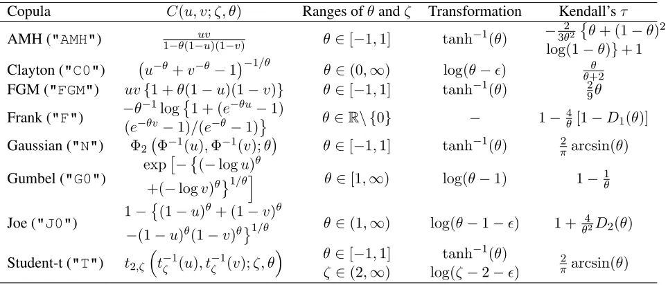
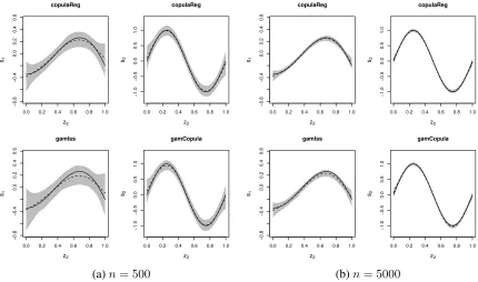
Figures 1 and 2 depict linear and non-linear estimates under the two methods whereas Table

3 reports the bias and root mean squared error of the parameter estimators. All mean estimates

are very close to the true values and, as expected, their variability decreases as the sample size

in-creases. Our proposal generally delivers less biased and more efficient estimates. The main

excep-tions are the estimates related to the copula parameter which are fairly close, withcopulaReg()

yielding slightly better results. Using a more complex function fors2(i.e.,_sin(6*pi*x)from

Vatter & Nagler (2016)) did not lead to different conclusions when comparing the two methods.

We also calculated95%average coverage probabilities for the smooth functions using point-wise

intervals based on the result of Section 2.4. The coverages delivered bycopulaReg() fors1

ands2 were 0.961 and0.943 forn = 500, and0.952 and0.956 forn = 5000, hence confirming

the good performance of the employed approximation.

We also explored whether the correct model is selected by AIC/BIC in the presence of several

−2

−1

0

1

βµ11 βµ12 βµ21 βν βθ

(a)n= 500

−2

−1

0

1

βµ11 βµ12 βµ21 βν βθ

(b)n= 5000

Figure 1: Linear coefficient estimates obtained by applyingcopulaReg()(black circles and black vertical bars) and the two-stage method by Vatter & Chavez-Demoulin (2015) (grey circles and grey vertical bars) to data simulated from Student-t copula models with inverse Gaussian (IG) and Singh-Maddala (SM) margins. The two stage approach is implemented usinggamlss()from the gamlss Rpackage for the margins andgamCopulafor the copula parameter. copulaReg() andgamlss+ gamCopulawere specified using the Student-t copula with IG and SM margins. Circles indicate mean estimates while bars represent the estimates’ ranges resulting from5%and95%

quantiles. True values are indicated by black solid horizontal lines.

0.0 0.2 0.4 0.6 0.8 1.0

−0.8 −0.4 0.0 0.2 0.4 0.6 copulaReg z2 s1

0.0 0.2 0.4 0.6 0.8 1.0

−1.0 −0.5 0.0 0.5 1.0 copulaReg z2 s2

0.0 0.2 0.4 0.6 0.8 1.0

−0.8 −0.4 0.0 0.2 0.4 0.6 gamlss z2 s1

0.0 0.2 0.4 0.6 0.8 1.0

−1.0 −0.5 0.0 0.5 1.0 gamCopula z2 s2

(a)n= 500

0.0 0.2 0.4 0.6 0.8 1.0

−0.8 −0.4 0.0 0.2 0.4 0.6 copulaReg z2 s1

0.0 0.2 0.4 0.6 0.8 1.0

−1.0 −0.5 0.0 0.5 1.0 copulaReg z2 s2

0.0 0.2 0.4 0.6 0.8 1.0

−0.8 −0.4 0.0 0.2 0.4 0.6 gamlss z2 s1

0.0 0.2 0.4 0.6 0.8 1.0

−1.0 −0.5 0.0 0.5 1.0 gamCopula z2 s2

(b)n= 5000

Figure 2: Smooth function estimates obtained by applying copulaReg()andgamlss+ gamCopulato data simulated from Student-t copula models with inverse Gaussian and Singh-Maddala margins. True functions are represented by black solid lines, mean estimates by dashed lines and pointwise ranges resulting from5%and95%

Bias RMSE

copulaReg gamlss+gamCopula copulaReg gamlss+gamCopula

n= 500 βµ11 0.070 0.000 0.650 0.911

βµ12 0.019 0.024 0.400 0.504

βµ21 -0.006 -0.018 0.137 0.235

βν 0.018 -0.030 0.080 0.108

βθ 0.029 -0.018 0.188 0.190

s1 0.021 0.035 0.084 0.117

s2 0.023 0.029 0.118 0.120

n= 5000 βµ11 0.017 -0.001 0.167 0.245

βµ12 0.002 0.002 0.110 0.146

βµ21 -0.002 -0.022 0.041 0.077

βν 0.004 -0.039 0.023 0.051

βθ 0.005 0.013 0.057 0.061

s1 0.008 0.017 0.029 0.043

s2 0.010 0.014 0.039 0.042

Table 3: Bias and root mean squared error (RMSE) obtained by applying the copulaReg() and gamlss +

gamCopulaparameter estimators to data simulated from Student-t copula models with inverse Gaussian and Singh-Maddala margins. Bias and RMSE for the smooth terms are calculated, respectively, asn−1

s

Pns

i=1|s¯ˆi −si| and

n−1

s

Pns

i=1

q

n−rep1Pnrep=1rep (ˆsrep,i−si)2, wheres¯ˆi =n−rep1

Pnrep

rep=1ˆsrep,i,nsis the number of equally spaced fixed

values in the(0,1)range, andnrepis the number of simulation replicates. In this case,ns= 200andnrep= 1000.

The bias for the smooth terms is based on absolute differences in order to avoid compensating effects when taking the sum.

non-correct copulae with one incorrect margin (i.e., Singh-Maddala was replaced with Weibull).

For each scenario and replicate, the correct model was always chosen by both criteria.

Finally, comparing the computation times of the two methods for the scenarios considered here

when using a 2.20-GHz Intel(R) Core(TM) computer running Windows 7, we generally found that

copulaRegis 1.3 times faster than gamlss + gamCopula. As for the latter approach, the

margins’ estimation step was the most expensive as it typically amounted to 93% of the total

computation time.

4

Empirical illustrations

The next sections illustrate the proposed bivariate copula additive modeling framework using two

empirical case studies based on electricity and birth data.

4.1

Analysis of Spanish electricity price and demand data

The aim of this section is to build an explanatory bivariate time-series model for electricity price

electricity prices throughout the time and one way of capturing this is via transfer function models

(e.g., Nogales & Conejo, 2006). Here, we take a different approach by relating price and demand

of energy using copulae. We also quantify the effect of prices of raw materials (oil, gas and

coal) on electricity price and demand. In the last decade, the issue of modeling electricity price

and demand has been the key question to determine the causes of price behavior as well as the

macroeconomic significance of the prices of raw materials, since Spain is an importer country. We

use working-daily data from January 1, 2002 to October 31, 2008 which are available from theR

packageMSwM(Sanchez-Espigares & Lopez-Moreno, 2014).

The first step is to choose the margins. Following the guidelines of Section 2.5, we choose the

normal and Gumbel distributions for price and demand, respectively. As for the choice of copula

we start off with the normal. We also allow the dependence between the margins, location and

scale parameters to vary with raw material prices. In addition to these covariates, we employ a

time variable as the underlying electricity prices and demands tend to vary with time, for reasons

which may have little or nothing to do with material prices. When we attempt to fit a copula model

in which all variables (time, oil, gas and coal prices) enter the five equations (two equations for the

location parameters, two for the scale parameters and one equation for the association parameter)

the algorithm fails to converge. This suggests that the sample size is perhaps low compared to the

complexity of the model. We, therefore, try out more parsimonious specifications. Specifically,

we always keep the time variable in all the model’s equations and, in a forward selection fashion,

choose the best (converged) model as judged by AIC and BIC. This leads to

eq.mu.1 <- Price ~ s(t, k = 60) + s(Oil) + s(Coal)

eq.mu.2 <- Demand ~ s(t, k = 60) + s(Oil) + s(Gas) + s(Coal)

eq.sigma2.1 <- ~ s(t, k = 60)

eq.sigma2.2 <- ~ s(t, k = 60) + s(Oil) + s(Gas)

eq.theta <- ~ s(t, k = 60)

fl <- list(eq.mu.1, eq.mu.2, eq.sigma2.1, eq.sigma2.2, eq.theta)

outN <- copulaReg(fl, margins = c("N", "GU"), data = energy, ...)

where thesare smooth functions of time, oil, gas and coal represented using penalized low rank

thin plate splines with default second order penalties andk(the number of basis functions) equal

to 10, unless otherwise stated; see SM-1 for more details. The value ofk = 60for the smooth

Peng & Dominici (2008), if k per year is small (say 2) then only the long-term trend and

sea-sonality are accounted for and other sub-seasonal and shorter-term variations remain in the data.

When building an explanatory time-series model, using 10 or 12 bases per year is more

appropri-ate as variation in the data longer than a timescale of about one week is modeled. As a sensitivity

analysis, we increased the kvalues for thes terms by several multiples of their original values;

the smooth functions of t became increasingly wigglier and the effects of raw material prices

progressively smoother. This suggested that allowing the time variable to capture very short

timescale variation in the data has a detrimental impact on the explanatory power of the model

(e.g., Peng & Dominici, 2008; Wood, 2006). The final estimated edfs for the smooth components

are57.7, 1, 6.6foreq.mu.1, 55.2, 8.4, 7.4, 8.8foreq.mu.2, 55.2foreq.sigma2.1, 53.6,

8.3, 7.4 for eq.sigma2.2, and 50.7 for eq.theta. Recall that when the edf is equal to 1,

the respective estimated effect is linear, hence the covariate can enter the model parametrically.

On the other hand, the higher the edf the more complex the estimated curve. The total number of

estimated parameter is 363 and the computation time was about 12 minutes. TheRcode used for

this analysis is given in SM-2.

The overall Kendall’s τˆandθˆare positive and significant (seesummary(outN)), however

some of the individualτˆandθˆassume negative values. We, therefore, tried all mixed combinations

of the Clayton, Gumbel and Joe families,T,F,AMHandFGMwhere the last two can only account

for weak dependencies (₋0.18≤ τ ≤ 0.33and₋0.22≤ τ ≤ 0.22, respectively). The Gaussian

copula is the most supported model by AIC and BIC. Using the Student-t copula virtually yielded

the same results as those obtained under the Gaussian copula; this did not come as a surprise as

the estimated value for theζ was249.15.

Marginal residual plots for the final model are shown in Figure 3 and suggest that the choice of

distribution for the first margin is sound, whereas that for the second margin is questionable as the

lower-tail residuals are off the reference line. Unfortunately, in this case, it was not possible to find

a better fitting distribution. Autocorrelation plots of the response variable and quantile residuals

(obtained after fitting the model) show that, while most of the structure has been modeled, short

term auto-correlation is still present in the data; see Figure 1 in SM-2. This could be addressed by

incorporating in the model autoregressive and/or moving average components but it is beyond the

Histogram and Density of Residuals

Quantile Residuals

Density

−3 −2 −1 0 1 2 3

0.0

0.1

0.2

0.3

0.4

−3 −2 −1 0 1 2 3

−3

−2

−1

0

1

2

3

Normal Q−Q Plot

Theoretical Quantiles

Sample Quantiles

Histogram and Density of Residuals

Quantile Residuals

Density

−4 −2 0 2

0.0

0.1

0.2

0.3

0.4

−3 −2 −1 0 1 2 3

−4

−3

−2

−1

0

1

2

3

Normal Q−Q Plot

Theoretical Quantiles

Sample Quantiles

year

θ

^

2002 2003 2004 2005 2006 2007 2008 2009

−0.5

0.0

0.5

1.0

Figure 4: Estimates and95%intervals forθover time from a Gaussian copula model with normal and Gumbel margins fitted to electricity price and demand data.

Using the fitted model, we build the plot in Figure 4 which shows that the correlation between

Price and Demand fluctuates around 0.5 (a similar plot could be produced for Kendall’s τ).

Many of the intervals do not contain zero: after accounting for raw material prices, a significant

association between the two responses which varies over time still persists. The reason of these

fluctuations are most likely due to variables, such as weather conditions and human habits, that

we could not control for because they were not available. Moving on to the covariate effects and

focusing, for instance, on the first equation, Figure 5 displays the impacts oft,OilandCoalon

Price. The plots show a cyclic trend with maximum and minimum peaks and suggest that on

average electricity price tends to linearly increase withOil, and decrease and then stabilize with

Coalalthough there is substantial uncertainty related to the last half of the curve. The estimated

effect ofCoalis counter-intuitive and further research is needed to shed light on this. Figure 2

in SM-2 reports the estimates and intervals for σ2

1. We could also predict joint and conditional

probabilities of interest from the model. This point is illustrated in the next section.

When we employed the two-stage estimation approach by Vatter & Chavez-Demoulin (2015),

the algorithm converged in about 16 minutes (after settingcontrol = gamlss.control(n.cyc

year

s(time

, 57.71)

2002 2003 2004 2005 2006 2007 2008 2009

−4

−2

0

2

4

20 40 60 80

−0.5

0.0

0.5

1.0

Oil

s(Oil,1)

40 60 80 100 140

−1.0

0.0

1.0

2.0

Coal

s(Coal,6.62)

above.

It would be interesting to compare the performance of bivariate and univariate GAMLSS in

a context of forecasting. However, this would make more sense if the models were specified

with this goal in mind. A possibility would be to follow the approach by Marx et al. (2010) and

Lee & Durban (2012) in which case the scope of the models would have to be extended

accord-ingly.

4.2

North Carolina birth data analysis

The analysis in this section uses 2010 birth data from the North Carolina Center for Health

Statis-tics (http://www.schs.state.nc.us/) which provides details on all the live births

oc-curred within the State of North Carolina, including information on infant and maternal health

and parental characteristics. The data cover maternal demographic information, pregnancy related

events and outcomes, maternal medical complications, newborn conditions and maternal health

behaviors. The choice of variables largely follows the work by Neelon et al. (2012) and the

anal-ysis reported below is for female infants (similar results were obtained for male infants). The

responses are birth weight in grams (bwgram) and gestational age in weeks (wksgest). The

co-variates are maternal ethnicity (nonhisp, categorized as non-Hispanic and Hispanic), singleton

birth (multbirth, born as a multiple or single birth), maternal age (magein years), mother’s

marital status (married) and county (county, indicating the North Carolina county of

resi-dence of the mother).

Birth weight and gestational age are important determinants of infant and child health;

re-cent evidence has also shown that these factors affect long-term health throughout adulthood

(Oreopoulos et al., 2008; Hack et al., 2002). Although both birth weight and gestational age are

predictors of future health, modelling these outcomes jointly is essential for a number of reasons.

First, birth weight and gestational age are highly correlated and confounded by factors such as

intrauterine growth restriction (Slattery & Morrison, 2002). In addition, risk factors for low birth

weight, such as maternal age, are also the same risk factors for preterm birth. Finally, evidence

suggests that the impact of low birth weight on health may be elevated by low gestational age, and

vice-versa (Hediger et al., 2002). Thus, modelling these outcomes independently would present a

more accurate picture is revealed by modelling these outcome jointly. The goal is, therefore, to

build a bivariate copula regression model for the simultaneous analysis ofbwgramandwksgest.

The resulting model can, for instance, be used to estimate the association (adjusted for covariates)

betweenbwgramandwksgestby county, to quantify the effects of covariates onbwgramand

wksgest, and to calculate joint and conditional probabilities of interest.

We first choose the marginal distributions forbwgramandwksgestbased on the guidelines

outlined in Section 2.5. The normal Q-Q plots of the normalized quantile residuals and AIC/BIC

suggest that the best fits for bwgram and wksgest are achieved using the logistic and

Gum-bel distributions (see Figure 3 in SM-4). Using backward selection, we fit bivariate models for

bwgramandwksgest and choose the best model as judged by AIC and BIC. Several copulae

are also tried out in a similar way as described in the previous section. The final model is

eq.mu.1 <- bwgram ~ nonhisp + multbirth + married + s(mage) +

s(county, bs = "mrf", xt = xt)

eq.mu.2 <- wksgest ~ nonhisp + multbirth + married + s(mage) +

s(county, bs = "mrf", xt = xt)

eq.sigma2.1 <- ~ nonhisp + multbirth + married + s(mage) +

s(county, bs = "mrf", xt = xt)

eq.sigma2.2 <- ~ multbirth + married + s(mage) +

s(county, bs = "mrf", xt = xt)

eq.theta <- ~ nonhisp + multbirth + s(mage) +

s(county, bs = "mrf", xt = xt)

fl <- list(eq.mu.1, eq.mu.2, eq.sigma2.1, eq.sigma2.2, eq.theta)

outC0 <- copulaReg(fl, margins = c("LO", "GU"), BivD = "C0",

data = datNC, ...)

where the default number of basis functions for the Gaussian Markov random field smooth term

(mrf) is equal to the number of covariate’s levels or regions (in this case, number of North

Car-olina counties which is 100), and a Clayton copula is used to join the logistic and Gumbel

distri-butions for the two responses. The first two equations refer to theµparameters ofbwgramand

wksgest, the third and fourth to theσ2 parameters and the last toθ. These parameters are

mod-eled using additive predictors involving factor, continuous and regional variables. The use ofmrf

smoothers in all equations ensures that the distribution parameters vary smoothly across counties.

The total number of observations and estimated parameters are 56940 and 558, respectively, and

af-fect the final result and only increased the computation time. The estimated edfs for the smooth

components are5.5, 52.0 for eq.mu.1, 4.3, 68.6 for eq.mu.2, 5.3, 3.9 for eq.sigma2.1,

2.6, 45.6foreq.sigma2.2, and5.3,36.6foreq.theta. Note that a low value for the edf of

themrf smooth term indicates that the estimated county effects are similar with each other and

vice-versa. TheRcode used for this analysis is given in SM-3.

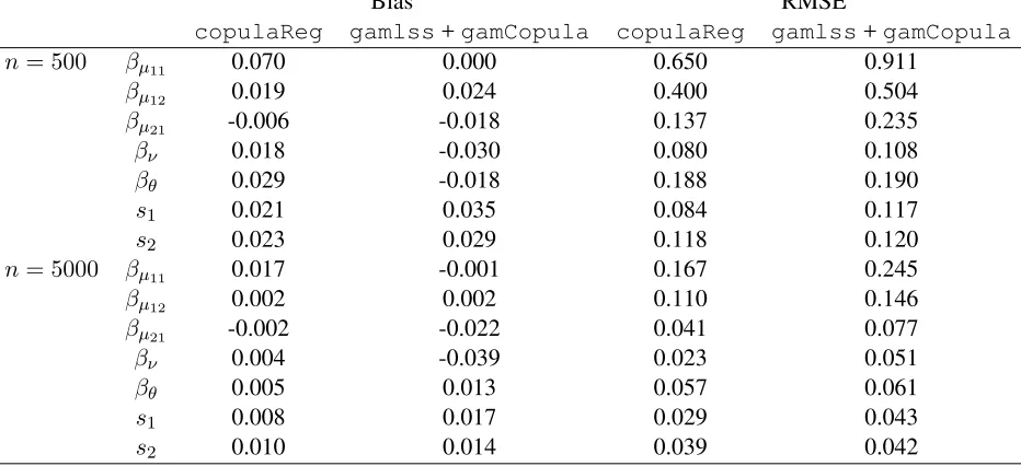
Figure 6 shows the joint probabilities of low weight birth babies and premature deliveries

in North Carolina when using a copula model and an independence model (which assumes that

bwgramanwksgestare not associated after accounting for covariates). This joint probability

was calculated for all the observations in the dataset and then averaged by county. The AIC/BIC

values for the copula and independence models suggest that the former provides a better fit to

the data. As it can be seen from Figure 6, in this case, assuming independence leads to smaller

probabilities. Looking at the copula model’s results, the probabilities vary across counties, ranging

from around 2% to 7%. The least favorable places to be born are clustered in the northeast of

the state, specifically Hertford, Northampton, Halifax, Edgecombe, Gates, Chowan, Perquimans,

Pasquotank, Camden, Currituck, Tyrell and Hyde counties.

For comparison purposes, we also employed the two stage approach with the same model

specification as that used forcopulaReg(). Computatio time was around 34 minutes where

the majority of time was spent at the margins’ stage. Results are similar to those obtained using

copulaReg()(see Figures 4, 5 and 6 in SM-4).

An analysis similar to that produced in Section 4.1, showing for instance some estimated

smooth function and Kendall’sτˆby county is given in SM-4 to save space.

5

Discussion

We have introduced a modeling framework for bivariate copula additive models for location, scale

and shape. The modularity of the estimation approach allows for easy inclusion of potentially any

parametric continuous marginal distribution and copula function as long as the cdfs and pdfs are

known and their derivatives with respect to their parameters exist. Parameter estimation is carried

out within a penalized maximum likelihood estimation framework with integrated automatic

mul-tiple smoothing parameter selection, and known and reliable inferential results from the smoothing

1

2

3

4

5

6

Joint probabilities (in %) from copula model

1

2

3

4

5

6

Joint probabilities (in %) from independence model

be easily used via copulaReg() inSemiParBIVProbit and the potential of the approach

has been demonstrated using simulated and real data.

Future releases of SemiParBIVProbit will incorporate more copulae and marginal

dis-tributions as well as facilities for comparing the predictive ability of competing models based,

for instance, on proper scoring rules (Gneiting & Raftery, 2007). Copula models with

binary-discrete, binary-continuous, discrete-discrete and discrete-continuous margins will also be made

available in the near future. These developments will obviously involve writing and implementing

the respective log-likelihood functions, score vectors and Hessian matrices, but the estimation and

inferential framework will essentially be unaffected by such changes.

Future research will look into the feasibility of strengthening the framework described in

this article by incorporating two-parameter and non-exchangeable copulae (e.g., Durante, 2009;

Frees & Valdez, 1998; Brechmann & Schepsmeier, 2013). Another interesting extension would

be to consider systems involving more than two responses using C- and D-Vine copulae (e.g.,

Brechmann & Schepsmeier, 2013).

Acknowledgement

We would like to thank two reviewers for their well thought out suggestions which improved

considerably the presentation and message of the article. One reviewer also provided very useful

comments onSemiParBIVProbit and asked us to implement the Student-t copula as well as

mixed versions of the Clayton, Gumbel and Joe families. Finally, we are indebted to Thibault

Vatter for various clarifications on the use ofgamCopula.

References

Acar, E. F., Craiu, V. R., & Yao, F. (2013). Statistical testing of covariate effects in conditional

copula models. Electronic Journal of Statistics, (pp. 2822–2850).

Brechmann, E. C. & Schepsmeier, U. (2013). Modeling dependence with c- and d-vine copulas:

The R package CDVine. Journal of Statistical Software, 52(3), 1–27.

Conn, A. R., Gould, N. I. M., & Toint, P. L. (2000). Trust Region Methods. Society for Industrial

and Applied Mathematics.

Dunn, P. K. & Smyth, G. K. (1996). Randomized quantile residuals. Journal of Computational

and Graphical Statistics, 5, 236–245.

Durante, F. (2009). Construction of non-exchangeable bivariate distribution functions. Statistical

Papers, 50, 383–391.

Fermanian, J. D. & Wegkamp, M. H. (2012). Time-dependent copulas. Journal of Multivariate

Analysis, 110, 19–29.

Frees, E. W. & Valdez, E. A. (1998). Understanding relationships using copulas. North American

Actuarial Journal, 2, 1–25.

Gentle, J. E. (2003). Random number generation and Monte Carlo methods. Springer-Verlag,

London.

Geyer, C. J. (2015). trust: Trust Region Optimization. R package version 0.1-6.

Gijbels, I., Veraverbeke, N., & Omelka, M. (2011). Conditional copulas, association measures

and their applications. Computational Statistics and Data Analysis, 55, 1919–1932.

Gilbert, P. & Varadhan, R. (2015).numDeriv: Accurate Numerical Derivatives. R package version

2014.2-1.

Gneiting, T. & Raftery, A. E. (2007). Strictly proper scoring rules, prediction, and estimation.

Journal of the American Statistical Association, 102, 359–378.

Gu, C. (1992). Cross validating non-gaussian data. Journal of Computational and Graphical

Statistics, 1, 169–179.

Gu, C. (2002). Smoothing Spline ANOVA Models. Springer-Verlag, London.

Hack, M., Flannery, D. J., Schluchter, M., Cartar, L., Borawski, E., & Klein, N. (2002).

Out-comes in young adulthood for very-low-birth-weight infants.New England Journal of Medicine,

Hastie, T. J. & Tibshirani, R. J. (1990). Generalized Additive Models. Chapman & Hall/CRC,

London.

Hediger, M. L., Overpeck, M. D., Ruan, W. J., & Troendle, J. F. (2002). Birthweight and

ges-tational age effects on motor and social development. Paediatric and Perinatal Epidemiology,

16(1), 33–46. 00140.

Kauermann, G., Schellhase, C., & Ruppert, D. (2013). Flexible copula density estimation with

penalized hierarchical b-splines. Scandinavian Journal of Statistics, 40, 685–705.

Klein, N. & Kneib, T. (2016). Simultaneous inference in structured additive conditional copula

regression models: a unifying bayesian approach. Statistics and Computing, 26(4), 841–860.

Klein, N., Kneib, T., Klasen, S., & Lang, S. (2015a). Bayesian structured additive distributional

regression for multivariate responses. Journal of the Royal Statistical Society, Series C, 64,

569–591.

Klein, N., Kneib, T., Lang, S., & Sohn, A. (2015b). Bayesian structured additive distributional

regression with an application to regional income inequality in germany. Annals of Applied

Statistics, 9(2), 1024–1052.

Kolev, N. & Paiva, D. (2009). Copula-based regression models: A survey. Journal of Statistical

Planning and Inference, 139, 3847–3856.

Kraemer, N. & Silvestrini, D. (2015). CopulaRegression: Bivariate Copula Based Regression

Models. R package version 0.1-5.

Kramer, N., Brechmann, E. C., Silvestrini, D., & Czado, C. (2012). Total loss estimation using

copula-based regression models. Insurance: Mathematics and Economics, 53, 829–839.

Lambert, P. (2007). Archimedean copula estimation using bayesian splines smoothing techniques.

Computational Statistics and Data Analysis, 51, 6307–6320.

Lee, D. J. & Durban, M. (2012). Seasonal modulation smoothing mixed models for time series

forecasting. Proceedings in the 27th International Workshop on Statistical Modelling, Prague,

Marra, G. & Radice, R. (2017). SemiParBIVProbit: Semiparametric Copula Bivariate Probit

Modelling. R package version 3.8-1.

Marra, G., Radice, R., Bärnighausen, T., Wood, S. N., & McGovern, M. E. (2017). A simultaneous

equation approach to estimating hiv prevalence with non-ignorable missing responses. Journal

of the American Statistical Association.

Marra, G. & Wood, S. (2012). Coverage properties of confidence intervals for generalized additive

model components. Scandinavian Journal of Statistics, 39, 53–74.

Marx, B. D., Eilers, P. H. C., Gampe, J., & Rau, R. (2010). Bilinear modulation models for

seasonal tables of counts. Statistics and Computing, 20(2), 191–202.

Neelon, B., Anthopolos, R., , & Miranda, M. L. (2012). A spatial bivariate probit model for

cor-related binary data with application to adverse birth outcomes. Statistical Methods in Medical

Research, 23(2), 119–133.

Nelsen, R. (2006). An Introduction to Copulas. New York: Springer, second edition.

Nocedal, J. & Wright, S. J. (2006). Numerical Optimization. New York: Springer-Verlag.

Nogales, F. J. & Conejo, A. J. (2006). Electricity price forecasting through transfer function

models. Journal of the Operational Research Society, 57, 350–356.

Oreopoulos, P., Stabile, M., Walld, R., & Roos, L. L. (2008). Short-, Medium-, and Long-Term

Consequences of Poor Infant Health An Analysis Using Siblings and Twins. Journal of Human

Resources, 43(1), 88–138. 00278.

Patton, A. J. (2002). Applications of copula theory in financial econometrics. Ph.D. thesis,

Uni-versity of California, San Diego.

Peng, R. D. & Dominici, F. (2008). Statistical Methods for Environmental Epidemiology with R:

A Case Study in Air Pollution and Health. Springer.

Radice, R., Marra, G., & Wojtys, M. (2016). Copula regression spline models for binary outcomes.

Rigby, R. A. & Stasinopoulos, D. M. (2005). Generalized additive models for location, scale and

shape (with discussion). Journal of the Royal Statistical Society, Series C, 54, 507–554.

Ruppert, D., Wand, M. P., & Carroll, R. J. (2003). Semiparametric Regression. Cambridge

University Press, New York.

Sabeti, A., Wei, M., & Craiu, R. V. (2014). Additive models for conditional copulas. STAT, 3,

300–312.

Sanchez-Espigares, J. A. & Lopez-Moreno, A. (2014).MSwM: Fitting Markov Switching Models.

R package version 1.2.

Segers, J., van den Akker, R., & Werker, B. J. M. (2014). Linear b-spline copulas with applications

to nonparametric estimation of copulas. Annals of Statistics, 42, 1911–1940.

Shen, X., Zhu, Y., & Song, L. (2008). Linear b-spline copulas with applications to nonparametric

estimation of copulas. Computational Statistics and Data Analysis, 52, 3806–3819.

Silverman, B. W. (1985). Some aspects of the spline smoothing approach to non-parametric

re-gression curve fitting. Journal of The Royal Statistical Society Series B, 47, 1–52.

Sklar, A. (1959). Fonctions de répartition é n dimensions et leurs marges.Publications de l’Institut

de Statistique de l’Université de Paris, 8, 229–231.

Sklar, A. (1973). Random variables, joint distributions, and copulas. Kybernetica, 9, 449–460.

Slattery, M. M. & Morrison, J. J. (2002). Preterm delivery. The Lancet, 360(9344), 1489–1497.

00704.

Stasinopoulos, M., Rigby, B., Voudouris, V., Akantziliotou, C., Enea, M., & Kiose, D. (2016).

gamlss: Generalised Additive Models for Location Scale and Shape. R package version 5.0-0.

Trivedi, P. K. & Zimmer, D. M. (2006). Copula Modeling: An Introduction for Practitioners.

Vatter, T. & Chavez-Demoulin, V. (2015). Generalized additive models for conditional dependence

structures. Journal of Multivariate Analysis, 141, 147–167.

Vatter, T. & Nagler, T. (2016). Generalized Additive Models for Pair-Copula Constructions.ArXiv