High Performance LDA through Collective Model
Communication Optimization
Bingjing Zhang
1, Bo Peng
1,2, and Judy Qiu
11 Indiana University, Bloomington, Indiana, U.S.A.
{zhangbj,pengb,xqiu}@indiana.edu
2 Peking University, Beijing, China
Abstract
LDA is a widely used machine learning technique for big data analysis. The application includes an inference algorithm that iteratively updates a model until it converges. A major challenge is the scaling issue in parallelization owing to the fact that the model size is huge and paral-lel workers need to communicate the model continually. We identify three important features of the model in parallel LDA computation: 1. The volume of model parameters required for local computation is high; 2. The time complexity of local computation is proportional to the required model size; 3. The model size shrinks as it converges. By investigating collective and asynchronous methods for model communication in different tools, we discover that optimized collective communication can improve the model update speed, thus allowing the model to converge faster. The performance improvement derives not only from accelerated communi-cation but also from reduced iteration computation time as the model size shrinks during the model convergence. To foster faster model convergence, we design new collective communi-cation abstractions and implement two Harp-LDA applicatons, “lgs” and “rtt”. We compare our new approach with Yahoo! LDA and Petuum LDA, two leading implementations favoring asynchronous communication methods in the field, on a 100-node, 4000-thread Intel Haswell cluster. The experiments show that “lgs” can reach higher model likelihood with shorter or similar execution time compared with Yahoo! LDA, while “rtt” can run up to 3.9 times faster compared with Petuum LDA when achieving similar model likelihood.
Keywords: Parallel Computing, LDA, Big Model, Communication Optimization
1
Introduction
z1,1
zi,j zi,1
Document Collection Topic assignment
x1,1
xi,j
xi,1
K*D
j
V*D
w
word-doc matrix
V*K
w
Nwk
word-topic matrix
≈
×
j
Mkj
topic-doc matrix
(a) (b)
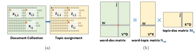
Figure 1: (a) Topics Discovery (b) View of Matrix Decomposition
We identify that the size of model required for local computation is so large that sending such data to every worker results in communication bottlenecks. The required computation time is great due to the large model size. In addition, the model size shrinks as the model converges. As a result, a faster communication method can speed up the model convergence, in which the model size shrinks and reduces the iteration execution time.
By guaranteeing the algorithm correctness, various model communication strategies are de-veloped in parallel LDA. Existing solutions favor asynchronous communication methods, since it not only avoids global waiting but also quickly makes the model update visible to other work-ers and thereby boosts the model convergence. We propose a more efficient approach in which the model communication speed is improved upon with optimized collective communication methods. We abstract three new communication operations and implement them on top of Harp [15]. We develop two Harp-LDA applications and compare them with Yahoo! LDA1and Petuum LDA2, two well-known implementations in the domain. This is done on three datasets each with a total of 10 billion model parameters. The results on a 100-node, 4000-thread Intel Haswell cluster show that collective communication optimizations can significantly reduce the communication overhead and improve the model convergence speed.
The following sections describe: the background of LDA application (Section 2), the big model problem in parallel LDA (Section 3), the model communication challenges in parallel LDA and related work (Section 4), Harp-LDA implementations (Section 5), experiments and performance comparisons (Section 6), and conclusion (Section 7).
2
Background
LDA modeling techniques can find latent structures inside the training data which are ab-stracted as a collection of documents, each with a bag of words. It models each document as a mixture of latent topics, and each topic as a multinomial distribution over words. Then an inference algorithm works iteratively until it outputs the converged topic assignments for the training data (see Fig. 1(a)). Similar to Singular Value Decomposition (SVD) (see Fig. 1(b)), LDA can be viewed as a sparse matrix decomposition technique on a word-document matrix, but it roots on a probabilistic foundation and has totally different computation characteristics.
Among the inference algorithms for LDA, Collapsed Gibbs Sampling (CGS) [12] shows high
1 https://github.com/sudar/Yahoo_LDA
[image:2.612.104.513.107.214.2]scalability in parallelization [3, 11], especially compared with another commonly used algorithm, Collapsed Variational Bayes (CVB3) [1]. CGS is a Markov chain Monte Carlo (MCMC) type
algorithm. In the “initialize” phase, each training data point, or token, is assigned to a random topic denoted aszij. Then it begins to reassign topics to each tokenxij =wby sampling from
a multinomial distribution of a conditional probability ofzij:
p zij =k|z¬ij, x, α, β∝
Nwk¬ij+β
P
wN
¬ij
wk +V β
Mkj¬ij+α (1)
Here superscript ¬ij means that the corresponding token is excluded. V is the vocabulary size. Nwk is the token count of word wassigned to topic kin K topics, andMkj is the token
count of topic k assigned in document j. The matrices Zij, Nwk and Mkj, are the model.
Hyperparameters α and β control the topic density in the final model output. The model gradually converges during the process of iterative sampling. This is the phase where the “burn-in” stage occurs and finally reaches the “stationary” stage.
The sampling performance is more memory-bound than CPU-bound. The computation itself is simple, but it relies on accessing two large sparse model matrices in the memory. In Algorithm. 1, sampling occurs by the column order of the word-document matrix, called “sample by document”. AlthoughMkj is cached when sampling all the tokens in a document
j, the memory access toNwk is random since tokens are from different words. Symmetrically,
sampling can occur by the row order, called “sample by word”. In both cases, the computation time complexity is highly related to the size of model matrices. SparseLDA [14] is an optimized CGS sampling implementation mostly used in state-of-the-art LDA trainers. In Line 10 of Algorithm. 1, the conditional probability is usually computed for each k with a total of K times, but SparseLDA decreases the time complexity to the number of non-zero items in one row ofNwk and in one column ofMkj, both of which are much smaller than K on average.
Algorithm 1:LDA Collapsed Gibbs Sampling Algorithm
input :training dataX, the number of topicsK, hyperparamtersα, β
output:topic assignment matrixZij, topic-document matrixMkj, word-topic matrixNwk 1 InitializeMkj, Nwk to zeros// Initialize phase
2 foreachdocumentj∈[1, D]do
3 foreachtoken positioni in documentj do
4 zi,j=k∼M ult(K1)// sample topics by multinomial distribution
5 mk,j += 1;nw,k+= 1// token xi,j is word w, update the model matrices // Burn-in and Stationary phase
6 repeat
7 foreachdocumentj∈[1, D]do
8 foreachtoken positioni in documentj do
9 mk,j −= 1;nw,k−= 1// decrease counts
10 zi,j=k0 ∼p(zi,j=k|rest)// sample a new topic by Eq.(1) 11 mk0,j += 1;nw,k0+= 1// increase counts for the new topic
12 untilconvergence;
3 CVB algorithm is used in Spark LDA ( http://spark.apache.org/docs/latest/mllib-clustering.html)
3
Big Model Problem in Parallel LDA
Sampling onZij in CGS is a strict sequential procedure, although it can be parallelized without
much loss in accuracy [3]. Parallel LDA can be performed in a distributed environment or a shared-memory environment. Due to the huge volume of the training documents, we focus on the distributed environment which is formed by a number of compute nodes deployed with a single worker process apiece. Every worker takes a partition of the training document set and performs the sampling procedure with multiple threads. The workers either communicate through point-to-point communication or collective communication.
LDA model contains four parts: I.Zij- topic assignments on tokens, II.Nwk - token counts
of words on topics (word-topic matrix), III.Mkj - token counts of documents on topics
(topic-document matrix), and IV.P
wNwk - token counts of topics. Here Zij is always stored along
with the training tokens. For the other three, because the training tokens are partitioned by document,Mkjis stored locally whileNwkandPwNwkare shared. For the shared model parts,
a parallel LDA implementation may use the latest model or the stale model in the sampling procedure. The latest model means the current model parameters used in computation are up-to-date and not modified simultaneously by other workers, while the stale model means the model parameters are old. We show that the model consistency is important to convergence speed in Section 6.
Now we calculate the size ofNwk, a huge but sparseV ∗K matrix. We note that the word
distribution in the training data generally follows a power law. If we sort the words based on their frequencies from high to low, for a word with ranki, its frequency isf req(i) =C∗i−λ. Then forW, the total number of training tokens, we have
W =
V X
i=1
f req(i) =
V X
i=1
(C∗i−λ)≈C∗(lnV +γ+ 1
2V) (2)
Hereλis a constant near 1, constantC=f req(1). To simplify the analysis, we considerλ= 1. ThenW is the partial sum of harmonic series which have logarithmic growth, where γ is the Euler-Mascheroni constant≈0.57721. The real model size (denoted asS) depends on the count of non-zero cells. In the “initialize” phase of CGS, with random topic assignment, a wordigets max(K, f req(i)) non-zero cells. Iff req(J) =K, thenJ =C/K, and we get:
Sinit= J X
i=1
K+
V X
i=J+1
f req(i) =W −
J X
i=1
f req(i) +
J X
i=1
K=C∗(lnV +lnK−lnC+ 1) (3)
The actual initial model sizeSinitis logarithmic to matrix sizeV∗K, which meansS << V∗K.
However this does not meanSinit is small. Since Ccan be very large, evenC∗ln(V ∗K) can
result in a large number. In the progress of iterations, the model size shrinks as the model converges. When a stationary state is reached, the average number of topics per word drops to a certain small constant ratio ofK, which is determined by the concentration parametersα,β and the nature of the training data itself.
The local vocabulary size V0 of each worker determines the model volume required for computation. When documents are randomly partitioned toN processes, every word with a frequency larger thanN has a high probability of occurring on all the processes. Iff req(L) = N at rank L, we get: L = W
(lnV+γ)∗N. For a large training dataset, the ratio between L
100 101 102 103 104 105 106 107
Word Rank
100 101 102 103 104 105 106 107 108 109 1010
Word Frequency
clueweb
y
= 10
9.9x
−0.9enwiki
y
= 10
7.4x
−0.8100 101 102 103 104
Document Collection Partition Number
0.0 0.2 0.4 0.6 0.8 1.0 1.2
Vocabulary Size of Partition (%)
clueweb
enwiki
(a) (b)
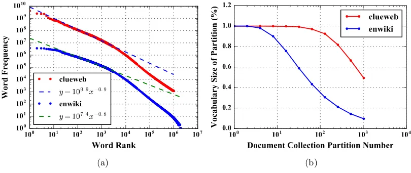
Figure 2: (a) Zipf’s Law of the Word Frequencies (b) Vocabulary Size vs. Document Partitioning
partitioning. When 10 times more partitions are introduced, there is only a sub-linear decrease in the vocabulary size per partition. We will use “clueweb” and “enwiki” datasets as examples (the contents of these datasets are discussed in Section 6). In “clueweb”, each partition gets 92.5% of V when the training documents are randomly split into 128 partitions. “enwiki” is around 12 times smaller than “clueweb”. It gets 90% ofV with 8 partitions, keeping a similar ratio. In summary, though the local model size reduces as the number of compute nodes grows, it is still a high percentage ofV in many situations.
4
Model Communication Challenges in Parallel LDA and
Related Work
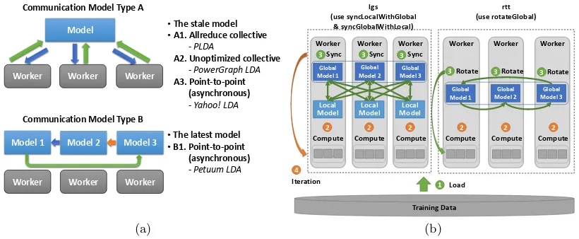
The analysis in previous sections shows three key properties of the big LDA model: 1. The initial model size is huge but it reduces as the model converges; 2. The model parameters required in local computation is a high percentage of all the model parameters; 3. The local computation time is related to the local model size. These properties indicate that model communication optimization is necessary because it can accelerate the model update process and result in a huge benefit in computation and communication of later iterations. Of the various communication methods used in state-of-the-art implementations, we abstract them into two types of communication models (see Fig. 3(a)).
In Communication Model Type A, the computation occurs on the stale model. Before performing the sampling procedure, workers fetch the related model parameters to the local memory. After the computation, they send updates back to the model. There are many com-munication models in this category. In A1, without storing a shared model, it synchronizes local model parameters through an “allreduce” operation [4]. PLDA [10] follows this communication model. “allreduce” is routing optimized, but it does not consider the model requirement in local computation, causing high memory usage and high communication load. In A2, model parameters are fetched and returned directly in a collective way. PowerGraph LDA4follows this communication model [6]. Though it communicates less model parameters compared with A1,
[image:5.612.102.507.108.279.2]Model
Worker Worker Worker
•The stale model •A1. Allreduce collective
-PLDA
A2. Unoptimized collective
-PowerGraph LDA
A3. Point-to-point (asynchronous) -Yahoo! LDA
Communication Model Type B Communication Model Type A
Worker Worker Worker
Model 1 Model 2 Model 3 ••The latest modelB1. Point-to-point
(asynchronous)
-Petuum LDA
Training Data 1 Load Worker Worker Worker
Sync
4
Global Model 2
Compute 2
Global Model 3
Compute 2
Global Model 1
Compute 2
3 3 Sync Sync
3
Iteration Local
Model ModelLocal ModelLocal
Worker Worker Worker
Rotate
Global Model 2
Compute 2
Global Model 3
Compute 2
Global Model 1
Compute 2
3 3 Rotate Rotate
3 lgs
(use syncLocalWithGlobal & syncGlobalWithLocal)
rtt (use rotateGlobal)
(a) (b)
Figure 3: (a) Communication Models (b) Harp-LDA Implementations
the performance is low for lack of routing optimization. A more popular communication model is A3, which uses asynchronous point-to-point communication. Yahoo! LDA [13, 2] and Pa-rameter Server [7] follow this communication model. In A3, each worker independently fetches and updates the related model parameters without waiting for other workers. A3 can ease the communication overhead, however, its model update rate is not guaranteed. A word’s model parameters may be updated either by changes from all the training tokens, a part of them, or even no change. A solution to this problem is to combine A3 and A2. This is implemented in Petuum (version 0.93) LDA [8].
In Communication Model Type B, each worker first takes a partition of the model param-eters, after which the model partitions are “shifted” between workers. When all the partitions are accessed by all the workers, an iteration is completed. There is only one communication model B1 which uses asynchronous point-to-point communication. Petuum (version 1.1) LDA [9] follows this model.
A better solution for Communication Model Type A can be a conjunction of A1 and A2 with new collective communication abstractions. There are three advantages to such a strategy. First, considering the model requirement in local computation, it reduces the model parameters communicated. Second, it optimizes routing through searching “one-to-all” communication patterns. Finally, it maintains the model update rate compared with asynchronous methods. For Communication Model Type B, using collective communication is also helpful because it maximizes bandwidth usage between compute nodes and avoids flooding the network with small messages, which is what B1 does.
5
Harp-LDA Implementations
Based on the analysis above, we parallelize LDA with optimized collective communication abstractions on top of Harp [15], a collective communication library plugged into Hadoop5. We use “table” abstractions defined in Harp to organize the shared model parameters. Each table may contain one or more model partitions, and the tables defined on different processes are
[image:6.612.102.512.107.276.2]associated to manage a distributed model. We partition the model parameters based on the range of word frequencies in the training dataset. The lower the frequency of the word, the higher the partition ID given. Then we map partition IDs to process IDs based on the modulo operation. In this way, each process contains model partitions with words whose frequencies are ranked from high to low.
We add three collective communication operations. The first two operations, “syncGlob-alWithLocal” and “syncLocalWithGlobal”, are paired. Here another type of table is defined to describe the local models. Each partition in these tables is considered a local version of a global partition according to the corresponding ID. “syncGlobalWithLocal” merges parti-tions from different local model tables to one in the global tables while “syncLocalWithGlobal” redistributes the model partitions in the global tables to local tables. Routing optimized broad-casting [4] is used if “one-to-all” communication patterns are detected. Lastly, “rotateGlobal” considers processes in a ring topology and shifts the model partitions from one process to the next neighbor.
We present two parallel LDA implementations. One is “lgs”, which uses “syncGlobalWith-Local” paired with “syncLocalWithGlobal”. Another is “rtt”, which uses “rotateGlobal” (see Fig. 3(b)). In both implementations, the computation and communication are pipelined, i.e., the model parameters are sliced in two and communicated in turns. Model Part IV is synchro-nized through A1 at the end of every iteration. SparseLDA algorithm is used for the sampling procedure. “lgs” samples by document while “rtt” samples by word. This is done to keep the consistency between implementations for unbiased communication performance comparisons in future experiments.
6
Experiments
Experiments are done on a cluster6 with Intel Haswell architecture. This cluster contains 32
nodes each with two 18-core 36-thread Xeon E5-2699 processors and 96 nodes each with two 12-core 24-thread Xeon E5-2670 processors. All the nodes have 128GB memory and are connected with 1Gbps Ethernet (eth) and Infiniband (ib). For testing, 31 nodes with Xeon E5-2699 and 69 nodes with Xeon E5-2670 are used to form a cluster of 100 nodes, each with 40 threads. All the tests are done with Infiniband through IPoIB support.
“clueweb”7, “enwiki” and “bi-gram”8 three datasets are used (see Table 1). The model parameter settings are comparable to other research work [5], each with a total of 10 billion parameters. αandβare both fixed to a commonly used value 0.01 to exclude dynamic tuning. We test several implementations: “lgs”, “lgs-4s” (“lgs” with 4 rounds of model synchronization per iteration, each round with 1/4 of the training tokens) and “rtt”. To evaluate the quality of the model outputs, we use the model likelihood on the training dataset to monitor model convergence. We compare our implementations with two leading implementations, Yahoo! LDA and Petuum LDA, and thereby learn how the communication methods affect LDA performance by studying the model convergence speed.
6.1
Model Convergence Speed Measured by Iteration
We compare the model convergence speed by analyzing model outputs on Iteration 1, 10, 20... 200. In an iteration, every training token is sampled once. Thus the number of model updates
6
https://portal.futuresystems.org
Dataset Num. of Num. of Vocabulary Doc Len. Num. of Init. Model
Docs Tokens AVG/STD Topics Size
clueweb 50.5M 12.4B 1M 224/352 10K 14.7GB
enwiki 3.8M 1.1B 1M 293/523 10K 2.0GB
[image:8.612.117.498.107.169.2]bi-gram 3.9M 1.7B 20M 434/776 500 5.9GB
Table 1: Training Data Settings in the Experiments
0 50 100 150 200
Iteration Number
1.4 1.3 1.2 1.1 1.0 0.9 0.8 0.7 0.6 0.5
Model Likelihood
1e11
lgs
Yahoo!LDA
rtt
Petuum
lgs-4s
0 50 100 150 200
Iteration Number
1.3 1.2 1.1 1.0 0.9 0.8 0.7 0.6 0.5
Model Likelihood
1e10
lgs
Yahoo!LDA
rtt
Petuum
(a) (b)
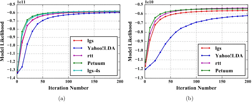
Figure 4: (a) Model Convergence Speed on “clueweb” (b) Model Convergence Speed on “enwiki”
in each iteration is equal. Then we see how the model converges with the same amount of model updates.
On “clueweb” (see Fig. 4(a)), Petuum has the highest model likelihood on all iterations. Due to “rtt”’s preference of using stale thread-local model parameters in multi-thread sampling, the convergence speed is slower. The lines of “rtt” and “lgs” are overlapped for their similar convergence speeds. In contrast to “lgs”, the convergence speed of “lgs-4s” is as high as Petuum. This shows that increasing the number of model update rounds improves the convergence speed. Yahoo! LDA has the slowest convergence speed because asynchronous communication does not guarantee all the model updates were seen in each iteration. On “enwiki” (see Fig. 4(b)), as before, Petuum achieves the highest accuracy out of all iterations. “rtt” converges to the same model likelihood level as Petuum at iteration 200. “lgs” demonstrates slower convergence speed but still achieves high model likelihood, while Yahoo! LDA has both the slowest convergence speed and the lowest model likelihood at iteration 200.
[image:8.612.104.509.221.391.2]0 5000 10000 15000 20000 25000
Execution Time (s)
1.4 1.3 1.2 1.1 1.0 0.9 0.8 0.7 0.6 0.5
Model Likelihood
1e11
lgs
Yahoo!LDA
lgs-4s
0 500 1000 1500 2000 2500 3000 3500
Execution Time (s)
1.3 1.2 1.1 1.0 0.9 0.8 0.7 0.6 0.5
Model Likelihood
1e10
lgs
Yahoo!LDA
(a) (b)
0 5000 10000 15000 20000 25000
Execution Time (s)
0 100 200 300 400 500 600 700 800
ExecutionTime Per Iteration (s)
lgs-iter
Yahoo!LDA-iter
lgs-4s-iter
0 500 1000 1500 2000 2500 3000 3500
Execution Time (s)
0 10 20 30 40 50 60 70 80
ExecutionTime Per Iteration (s)
lgs-iter
Yahoo!LDA-iter
[image:9.612.101.509.108.438.2](c) (d)
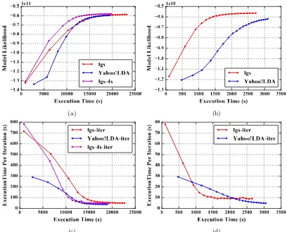
Figure 5: Model Likelihood vs. Elapsed Time on (a) “clueweb” (b) “enwiki”; Iteration Time vs. Elapsed Time on (c) “clueweb” (d) “enwiki”
6.2
Model Convergence Speed Measured by Elapsed Time
We first compare the execution speed between “lgs” and Yahoo! LDA. On “clueweb”, we show the convergence speed based on elapsed execution time (see Fig. 5(a)). Yahoo! LDA takes more time to finish Iteration 1 due to its slow model initialization, which demonstrates that it has a sizable overhead on the communication end. In later iterations, while “lgs” converges faster, Yahoo! LDA catches up after 30 iterations. This observation can be explained by our slower computation speed. To counteract the computation overhead, we increase the number of model synchronization rounds per iteration to four. Thus the computation overhead is reduced by using a newer and smaller model. Although the execution time for “lgs-4s” is still slightly longer than Yahoo! LDA, it obtains higher model likelihood and maintains faster convergence speed during the whole execution.
0 1000 2000 3000 4000 5000 6000 7000 8000
Execution Time (s)
1.4 1.3 1.2 1.1 1.0 0.9 0.8 0.7 0.6 0.5
Model Likelihood
1e11rtt
Petuum
0 1000 2000 3000 4000 5000 6000 7000
Execution Time (s)
0 50 100 150 200 250
ExecutionTime Per Iteration (s)
rtt-compute
rtt-iter
Petuum-compute
Petuum-iter
(a) (b)
1 2 3 4 5 6 7 8 9 10
Iteration
0 50 100 150 200 250 300ExecutionTime Per Iteration (s)
181 131 121 116 112 106 100 92 85 80 57 23 21
18 19 18
17 18
16 15 59 54 52
50 48 44 42 39 36 35 33
30 28 32 29
29 31 29 30 26
rtt-compute
rtt-overhead
Petuum-compute
Petuum-overhead
191 192 193 194 195 196 197 198 199 200
Iteration
0 5 10 15 20 25 30 35ExecutionTime Per Iteration (s)
23 23 23 23 23 23 23 23 23 23 3 3 3 2 3 3 3 2 3 3
19 19 19 19 19 19 19 19 19 19 10 10 10 11 9 10 9 9 10 10
rtt-compute
rtt-overhead
Petuum-compute
Petuum-overhead
[image:10.612.102.510.108.441.2](c) (d)
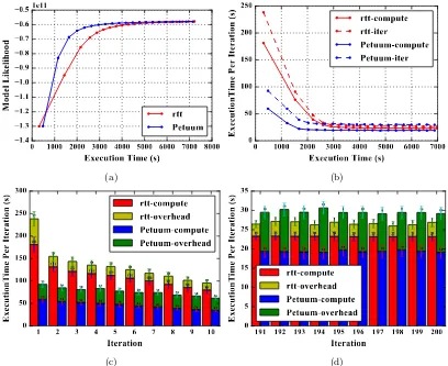
Figure 6: Comparison on “clueweb” (a) Model Likelihood vs. Elapsed Time (b) Iteration Time vs. Elapsed Time’ (c) First 10 Iteration Times (d) Final 10 Iteration Times
collective communication optimization, the model size quickly shrinks so that its computation time is reduced significantly. At the same, although Yahoo! LDA does not have any extra overhead other than computation in each iteration, its iteration execution time reduces slowly because it keeps computing with an older model (see Fig. 5(c)(d)).
0 1000 2000 3000 4000 5000 6000
Execution Time (s)
2.4 2.3 2.2 2.1 2.0 1.9 1.8 1.7
Model Likelihood
1e10
rtt
Petuum
0 1000 2000 3000 4000 5000 6000
Execution Time (s)
0 20 40 60 80 100 120
ExecutionTime Per Iteration (s)
rtt-compute
rtt-iter
Petuum-compute
Petuum-iter
(a) (b)
1 2 3 4 5 6 7 8 9 10
Iteration
0 20 40 60 80 100 120
ExecutionTime Per Iteration (s)
28 16
12 11 10
9 8 7 7 6 71
38 31
29
36 36
27 25 25 25
7 7 7 7 6 6 6 6 6 6 110
87 84
82 81 86 86 85 102
84
rtt-compute
rtt-overhead
Petuum-compute
Petuum-overhead
53 54 55 56 57 58 59 60 61 62
Iteration
0 20 40 60 80 100
ExecutionTime Per Iteration (s)
4 4 4 4 4 4 4 4 4 4 19 20 21 21 19 19 19 19 19 206 6 6 6 6 6 6 6 6 6 82 86 86 84 86 81 86 87 83
88
rtt-compute
rtt-overhead
Petuum-compute
Petuum-overhead
[image:11.612.102.509.107.442.2](c) (d)
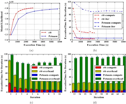
Figure 7: Comparison on “bi-gram” (a) Model Likelihood vs. Elapsed Time (b) Iteration Time vs. Elapsed Time (c) First 10 Iteration Times (d) Final 10 Iteration Times
Petuum cannot even continue executing after 60 iterations due to a memory outage (see Fig. 7(a)). Fig. 7(b)(c)(d) shows this performance difference on communication.
7
Conclusion
overhead than Petuum LDA, and the total execution time of “rtt” is 3.9 times faster. On “clueweb”, although the computation speed of the first iteration is 2- to 3-fold slower, the total execution time remains similar.
Despite the implementation differences between “rtt”, “lgs”, Yahoo! LDA, and Petuum LDA, the advantages of collective communication methods are evident. Compared with asyn-chronous communication methods, collective communication methods can optimize routing be-tween parallel workers and maximize bandwidth utilization. Though collective communication will result in global waiting, the resulting overhead is not as high as speculated. The chain reac-tion set off by improving the LDA model update speed amplifies the benefits of using collective communication methods. In future work, we will focus on improving intra-node LDA perfor-mance in many-core systems and apply our model communication strategies to other machine learning algorithms facing big model problems.
Acknowledgments
We gratefully acknowledge support from Intel Parallel Computing Center (IPCC) Grant, NSF 1443054 CIF21 DIBBs 1443054 Grant, and NSF OCI 1149432 CAREER Grant. We appreciate the system support offered by FutureSystems.
References
[1] D. Blei, A. Ng, and M. Jordan. Latent Dirichlet Allocation. The Journal of Machine Learning
Research, 3:993–1022, 2003.
[2] A. Ahmed et al. Scalable Inference in Latent Variable Models. InWSDM, 2012.
[3] D. Newman et al. Distributed Algorithms for Topic Models. The Journal of Machine Learning
Research, 10:1801–1828, 2009.
[4] E. Chan et al. Collective Communication: Theory, Practice, and Experience. Concurrency and
Computation: Practice and Experience, 19(13):1749–1783, 2007.
[5] E. Xing et al. Petuum: A New Platform for Distributed Machine Learning on Big Data. InKDD,
2015.
[6] J. Gonzalez et al. PowerGraph: Distributed Graph-Parallel Computation on Natural Graphs. In
OSDI, 2012.
[7] M. Li et al. Scaling Distributed Machine Learning with the Parameter Server. InOSDI, 2014.
[8] Q. Ho et al. More Effective Distributed ML via a Stale Synchronous Parallel Parameter Server.
InNIPS, 2013.
[9] S. Lee et al. On Model Parallelization and Scheduling Strategies for Distributed Machine Learning.
InNIPS, 2014.
[10] Y. Wang et al. PLDA: Parallel Latent Dirichlet Allocation for Large-scale Applications. In
Algorithmic Aspects in Information and Management, pages 301–314. 2009.
[11] Y. Wang et al. Peacock: Learning Long-Tail Topic Features for Industrial Applications. ACM
Transactions on Intelligent Systems and Technology, 6(4), 2015.
[12] P. Resnik and E. Hardist. Gibbs Sampling for the Uninitiated. Technical report, University of Maryland, 2010.
[13] A. Smola and S. Narayanamurthy. An Architecture for Parallel Topic Models. Proceedings of the
VLDB Endowment, 3(1-2):703–710, 2010.
[14] L. Yao, D. Mimno, and A. McCallum. Efficient Methods for Topic Model Inference on Streaming
Document Collections. InKDD, 2009.