The Most Recent Common Ancestor of a Randomly Chosen Sample in a Galton Watson Process

(1)

The Most Recent Common

Ancestor of a Randomly Chosen

Sample in a Galton-Watson

Process

A thesis submitted in partial fulfilment of the

requirements for the degree of Master of

Mathematical Sciences (Advanced)

by

Albert Christian Soewongsono

Supervisor

A/Prof. Conrad Burden

Mathematical Sciences Institute ANU College of Science The Australian National University

(2)

Declaration

This thesis is an account of research conducted between February 2018 and and October 2018 at the Mathematical Science Institute, The Australian National University, Canberra, Australia.

Except where acknowledged in the customary manner, the material presented in this thesis is, to the best of my knowledge, original and has not been submitted in whole or part for a degree in any university.

(3)

Acknowledgements

I would first like to thank my thesis supervisor A/Prof. Conrad Burden to guide me towards the completion of my thesis. His guidance throughout the year has helped me to build a good understanding of the subject. His office door was always open whenever I ran into a trouble spot or had questions about my re-search. He consistently allowed this paper to be my own work, but steered me in the right direction whenever he thought I needed it.

(4)

Abstract

One of the interesting topics to be examined in the field of theoretical population genetics is to find the most recent common ancestor of the current population. In this thesis, firstly we proceed by finding the common ancestor of two randomly chosen individuals at the current times, thus we will build a mathematical model to illustrate this situation using a Galton-Watson process which allows the pop-ulation to grow stochastically over time, and only genetic drift affects the model. We then generalise the model into modelling the common ancestor for n ran-domly chosen individuals at the current time step. Later, we derive the joint estimate of having a common ancestor fromn chosen individuals and the current population at time s does not exceed the observed population. Hence, this will be used to determine the estimate of the initial population size and the time of the most recent common ancestor for the case of n = 2. Lastly, we will compare the coalescent time with result found by Slatkin and Hudson (1991) using the Wright-Fisher model.

Keywords:Population Genetics, Most Recent Common Ancestor,

(5)

List of Notations

m0 = The initial population size.

κ0 = The scaled initial population size.

t= The continuous time step.

s= The scaled continuous time step.

τ = The discrete time step.

E2 = Event that two randomly chosen individuals at the current time

are descended from a common ancestor at times = 0.

En= Event that n randomly chosen individuals from a fraction xof the

current population at times descended from a common ancestor

at times= 0.

κ= The observed scaled current population size.

Z(s) = The population size at time s.

κ(s) = The scaled population size at time s.

κ1 = Sub-population of κ which is direct descendants from one individual

at time 0.

κ2 = Sub-population of κ which is descendants from m0−1 individuals

at time 0.

log λ= Per generation growth rate.

Π0(s, κ0, x0) = The extinction probability of the fraction x0 of the initial population

before times.

u(s, κ0) = Probability of having single ancestor from a sample of size n from

the current population at time s.

v(s, κ0) = Probability that the population at time s will not exceed the observed

current population given the starting population κ0.

L(s, κ0|κ) = The likelihood function that the population at time s will not exceed

the observed population κ for a given starting population κ0.

(6)

Chapter 1 Population Genetics: A Quick

Look

First introduced in 1920’s and 1930’s by Fisher, Haldane, and Wright, Popula-tion Genetics occupies a major role in understanding of evoluPopula-tionary processes of plants and animals important to mankind (Ewens (2004)). As the main concerns of this subject are the genetic differences within populations and the dynamics of how populations evolve throughout time as a result of genetic mutations hap-pening in the germlines1 _{of individuals (Gillespie (2004)), the study itself cannot}

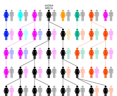
be separated of what is known as “Genetic Drift”. The genetic drift occurs when a single individual is the ancestor of a significant portion of the population in a subsequent population (See fig.4.1). Therefore, to understand the importance of genetic drift in determining the make up of a current population, it is useful to understand the statistical properties of the “Most Recent Common Ancestor” (MRCA) of a random sample of the population.

More specifically, one may want to estimate the time since the MRCA and the size of the population at that time. This is where mathematical modelling is required. As pioneers on this subject, the Wright-Fisher (W-F) model is the first to set foot on the study of the subject, and has ever since become the most com-monly used model on researches in this area. The W-F model is popular because it is relatively easy to study the ancestry of a sample of individuals, since it natu-rally ‘looks backwards’ in time i.e. each individual randomly chooses their parent.

However, this model has disadvantages of not being a good physical

(9)

tion of how populations propagate and it does not allow for a stochastically variable population size. On the other hand, the Galton-Watson (G-W) model is a closer description of reality since each individual randomly chooses the number of offspring. For a G-W model, populations evolve according to a common prob-ability distribution for the number of offspring of each parent on the assumption that this distribution is identical but independent for the whole population and throughout generations (O’Connell (1995); Cyran and Kimmel (2010)). In a later chapter, we will discuss this model more thoroughly and its features, including its diffusion limit via Forward-Kolmogorov equation.

(10)

3

Chapter 2 The Wright-Fisher Model: A

Brief Introduction

Introduced by Sewall Wright and Ronald Fisher (Neither of whom published the statement for the model, but did publish series of publications regarding the model) in 1931, the W-F model is the earliest model to deeply study Population Genetics and has been long considered important as the starting point for many researches in the field (Ewens (2004)). Although being the earliest model in the field, its assumption for constant population size i.e. no stochastic influence on the size of populations makes it biologically unrealistic, as for example, it cannot capture a growing population such as human populations (Burden and Simon (2016)). Based on the Binomial distribution, we shall discuss the model more deeply in later section. Since the main focus of this paper is on genetic drift, we will focus mainly on models without mutation or selection, including the W-F Model.

The Wright-Fisher model is constructed under the following assumptions:

• Non-Overlapping Generations: Imagine an annual plant where in each

season, new seeds replace the old ones. This assumes each individual in a

population in a given generation reproduce within discrete time stepτ and

τ + 1, whereτ ∈ {1,2,3,· · · }.

• Fixed Population Size: This assumes the population of size M remains

constant throughout generations.

• Diploid Population: This assumes that each individual in a population

(11)

population size M = 2N copies of genome, where N is the number of diploid individuals. An example of a diploid population is Clarkia plants.

• Monoecious Population: This assumes that each individual in a

popu-lation carries both male and female reproductive organs. Hence, a mating can occur between two individuals or within an individual. In fact, many plants are monoecious.

• Random Mating: This assumes that each individual in generationτ + 1

is offspring of two randomly chosen and independent individuals in gener-ation τ. Since the population is monoecious, both parents might be the same individual, therefore the probability of having one parent in previous generation is 1

M.

To start the construction of the model, given an observed SNP1, we shall ex-amine the model in which two distinct alleles2 A1, A2 ∈ {A, C, G, T}3 _{are present.}

Next, we define the random variable Y(τ) as the number of copies of allele A1

within the population at the time step or generation τ. It follows that its range is given by ΩY(τ) = {0,1,· · · , M}. Since the population is constant over

gen-erations and random mating is allowed, the number of copies of allele i in the population at the generationτ+ 1 is dependent only on the previous generation. Thus, it follows what is known as “Markov Processes”. Hence, we can define the transition probability for number ofA1 allele copies of the population going from generation τ to generation τ+ 1 as follows:

pij = Prob (Y(τ + 1) =j|Y(τ) =i), (2.1)

where Y(τ + 1) = j|Y(τ) = i ∼ Bin M,_Mi . Following the assumptions, the probability that any j individuals with allele type A1 at generation τ + 1 being

the offspring from i parents in the previous generation is _Mi . Consequently, the probability that the rest of current populationM−Yα{τ}inherit the other allele

type is 1− i

M. Thus,

pij =

M j

i M

j

1− i

M

M−j

. (2.2)

1_{Single Nucleotide Polymorphisms} _{or SNPs are the most common type of genetic variation.} 2_{Common term used in Population Genetics to describe different variants at a genetic locus.} 3_{Acronyms for 4 different types of Nucleobases:} _A _=Adenine, _C _=Cytosine,

(12)

It follows immediately from Eq. (2.2) that;

p0j =   

0 if j 6= 0 1 if j = 0

, pM j =   

0 if j 6=M,

1 if j =M.

(2.3)

This implies that 0 and M are the absorbing states of the model. In other words, these states correspond to situation where the population has either allele

A1 or allele A2 fixed. Hence, this gives rise to a question regarding the fixation

probabilities of both alleles in a long run.

2.1 Allele Fixation Probability in Wright-Fisher

Model with No Mutations

To begin with, let’s assume there are i number of copies of allele A1 within the

population at time τ = 0 i.e. Y(0) =i, where i ∈ {0,1,· · ·, M}. Then, first we would like to seek the probability of fixation of alleleA1 which can be interpreted

as;

Prob (AlleleA1 is fixed|Y0 =i) = Prob (Y(∞) =M|Y0 =i). (2.4)

Since this whole thing is a Markov Process, we can impose “the law of total probability” onto Eq. (2.4) to break it into sum of different cases as follows;

Prob (Y(∞) = M|Y(0) = i)

=

M X

j=1

Prob (Y(∞) =M|Y(1) =j) Prob (Y(1) =j|Y(0) =i). (2.5)

From Eq. (2.3), we know that 0 and M are the absorbing states. It follows immediately that the boundary conditions of the model are as follows;

Prob (Y(∞) =M|Y(0) = 0) = 0, Prob (Y(∞) = M|Y(0) =M) = 1.(2.6) By defining Ψi = Prob (Y(∞) =M|Y(τ) =i), we can rewrite Eq. (2.5) and

Eq. (2.6) as follows;

Ψi = M X

j=1

pijΨj, Ψ0 = 0,ΨM = 1. (2.7)

It is easy to check that the solution to Eq. (2.7) is;

Ψi =

i

(13)

Similarly, by replacing the boundary conditions to Ψ0 = 1 and ΨM = 0, the

(14)

Chapter 3 Galton-Watson Process in

Population Genetics

We will discuss briefly the G-W process, and subsequently build a story that will lead us to the main discussion of this thesis, which is finding the MRCA of a sample of a growing population. Since no mutations are involved in this thesis, we will proceed this discussion for the no-mutation model of G-W process.

3.1 A Brief Historical Review

Named after British mathematician and statistician Francis Galton and fellow British mathematician Henry William Watson, this term refers to Francis Gal-ton’s statistical investigation on the extinction of family names, particularly con-cerning the extinction of the Victorians’ aristocratic surnames. This problem was posed by Galton through the 1873 series of The Educational Times regarding the probability of such an event. At the same year, just a few months later, Watson replied to the problem issued by Galton also through The Educational Times with a solution, in which Galton described as “totally erroneous”. A year later, they published a joint paper (Galton and Watson, 1875) with the correct solution.

The main foundation of the model the two developed on their paper is by assuming that surnames would only be passed onto male children by their father, then by supposing the number of a man’s sons as a discrete random variable say,

Yα where Yα ∈ {0,1,2,· · · }they again assumed that different men’s sons are all

(15)

with a particular surname at the next generation τ+ 1, M(τ+ 1), can be defined as

M(τ + 1) =

M(τ)

X α=1

Yα.

From here we can see that this forms a stochastic process which only depends on exactly one previous generation. The conclusion drawn from this is that if the expected number of a man’s sons is less than one, i.e E(Yα) ≤ 1 then their

surname will go extinct ”almost surely”1_{, while if its expectation is more than}

one, then there is probability that the inherited surname will survive in any given number of generations (Galton and Watson, 1875). Their work was actually inde-pendent of an earlier similar result found but unpublished by French Statistician I.J. Bienaym´e.

The branching model has many applications in various research fields, such as understanding human Y-chromosome DNA haplogroups2 _{(Kendall, 1966),}

un-derstanding Nuclear Chain Reaction (Byers, 2002), and in the field of Population Genetics, was used by Burden and Simon (2016) to study Mitochondrial Eve 3_.

The latter will also be discussed on this paper in later section as a building block to lead us to the main discussion of this paper.

3.2 The Derivation of The Model

We shall start by stating all the assumptions used for developing G-W Branching Process. Those assumptions are as follows:

• The population size is not fixed, but rather varying stochastically.

• Consider a population ofM(τ) haploid individuals at generationτ in which every individual in the population reproduce in discrete,non-overlapping, independent generations τ = 1,2,3,· · ·.

• The population is grouped intondifferent allele types such that the number

1_{It is terminology in Probability Theory to describe that an event which occurs with}

prob-ability 1, even though the complementary event is, in principle, possible.

2_{It is a group of genes inherited from a single parent in which mutations occurred in the}

non-recombining portions of the DNA from the Y-chromosome.

(16)

of sub-population with allele type η is Yη(τ). Thus,

M(τ) =

n X

i=1

Yi(τ). (3.1)

• No mutations between allele types nor selection occur.

• The number of offspring per individuals with allele typeηin any generation is a set of independent and identically distributed (i.i.d.) random variables

S_i(η), i= 1,· · · , Yη(τ). Since they are identical, we will denote from now on

a non-negative integer valued random variableS having mean and variance denoted by;

E(S) = λ, Var(S) =σ2. (3.2)

Since λ and σ2 _{are common to all allele types, the process can be thought of as}

modelling a population subject to genetic drift but not mutation or selection. It is clear that;

Yη(τ + 1) = Yη(τ)

X i=1

S_i(η). (3.3)

Hence, using the formula for the mean of the sum of a random number of i.i.d. random variables,

E(Yη(τ+ 1)) =E  

Yη(τ)

X i=1

S_i(η)

 

=E(Yη(τ))E

S_i(η)

=E(Yη(τ))E(S)

=λE(Yη(τ)). (3.4)

Suppose we have initial conditions given as follows;

Yη(0) =yη, M(0) =m0 =

n X

i=1

Yi(0). (3.5)

It, then, follows immediately from Eq. (3.1) and Eq. (3.4) that;

(17)

3.3 The Continuum Galton-Watson Process Via

the Forward Kolmogorov Equation

We will examine the diffusion limit of the G-W branching model using the Forward-Kolmogorov equation 4_.

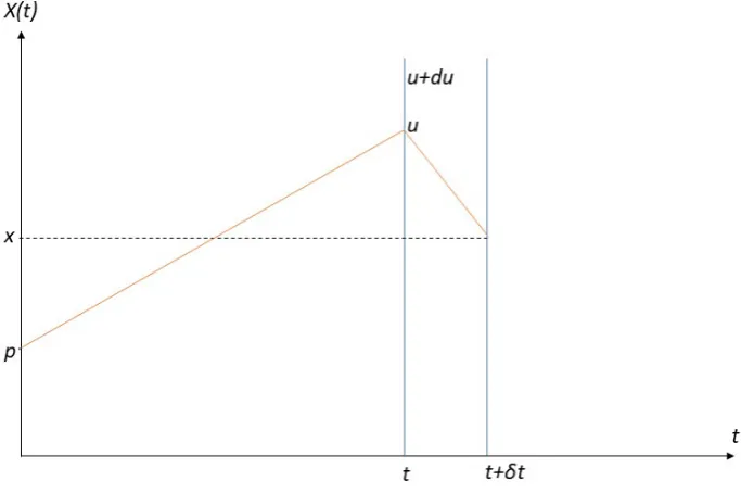
The main reason we need to look into its continuum model is because, nat-urally, the population size is generally large, especially human population. This continuum approach of the G-W model has been discussed in detail by Feller (1951) and is summarised by Bailey (1964) and Cox and Miller (1978). We will specify only for the case of 2 alleles, therefore we will start by stating that Y(τ) to be the number of copies or sub-population of allele type A1. These following

changes are made to accommodate the model:

t= τ

m0

X(t) = 1

MY(τ) x0 = y0 m0

=p ”Scaled initial population” (3.7)

δt= 1

M δX(t) =

1

M [Y(τ+ 1)−Y(τ)]. (3.8)

In Appendix 7.3 we assume the existence of the functionsa(x) andb(x) defined by Eq. (7.8), thus we will find what a(x) and b(x) correspond to in the Galton-Watson process. As noted in Burden and Simon (2016), the continuum limit is obtained under assumptions m0 → ∞ and λ → 1 such that the growth rate α=m0logλ remains constant.

4_{Also known as Fokker-Planck equation in Physics, it is a partial differential equation that}

(18)

Then,

E(δX(t)|X(t) =x) = 1

m0

E(Y(τ + 1)−Y(τ)|Y(τ) = y)

= 1

m0

[E(Y(τ + 1)|Y(τ) =y)−E(Y(τ)|Y(τ) =y)]

= 1

m0

[λE(Y(τ)|Y(τ) = y)−y]

= 1

m0

(λy−y)

= 1

m0

(λ−1)y

= 1

m0

(λ−1)xm0

=αxδt+O(δt2). (3.9)

Therefore,

a(x) = αx. (3.10)

Then, to determine b(x), let’s examine the following;

E δX(t)2|X(t) =x

=Var (δX(t)|X(t) =x) +E(δX(t)|X(t) =x)2 =Var (δX(t)|X(t) =x) + (αxδt+O(δt))2 =Var (δX(t)|X(t) =x) +O δt2

= 1

m2 0

Var (Y(τ + 1)−Y(τ)|Y(τ) =y) +O δt2

= 1

m2 0

[Var (Y(τ+ 1)−y|Y(τ) = y)]

= 1

m2 0

Var (Y(τ + 1)|Y(τ) = y) +O δt2

= 1

m2₀yσ

2₊_{O δt}2

= 1

m0

xσ2 +O δt2

=σ2xδt+O δt2. (3.11)

Therefore,

(19)

Substitute these back to Eq. (7.18) in Appendix 7.3, we get the corresponding Forward-Kolmogorov equation for the Galton-Watson process as follows:

∂f

∂t =−α ∂

∂x(xf(x, t)) +

1 2σ

2 ∂2

∂x2 (xf(x, t)). (3.13)

The solution of the above equation forα6= 0 and the initial conditionf(x,0) =

δ(x−x0), as shown in Bailey (1964) is the following; (See Appendix 7.4 for a

derivation)

f(x, t) = 2α

σ2₍_eαt₋₁₎

x0eαt x

1₂

exp

₋

2α(x0eαt+x) σ2₍_eαt₋₁₎

I1

4α(x0xeαt)

1 2

σ2₍_eαt₋₁₎ !

+δ(x)p0(t), (3.14)

whereI1 is theModified Bessel Function (See Appendix 7.2) of the first kind,δ(x) is the Dirac Delta function (See Appendix 7.1), and the extinction probability given by (Bailey, 1964),

p0(t) = exp

₋

2αx0eαt σ2₍_eαt₋₁₎

. (3.15)

Note that the term involving the delta function in Eq. (3.14) corresponds to a point mass at zero which indicates that the given allele type becomes extinct at or before time t (Burden and Simon, 2016). Furthermore, the limiting cases for the extinction probability are given by;

lim

t→∞p0(t) =

  

1 if α≤0

e

−2αx₀

σ2 if α >0

. (3.16)

(20)

Chapter 4 Earlier Results in the

Application to Mitochondrial Eve

Since centuries ago, many researches have been undertaken among scientists to determine the origin of humankind. One of the most discussed one is to find the

mitochondrial Eve1_{or the most recent common ancestor (MRCA) of all currently}

living humans following the maternal line (See Fig.4.1).

The male counterparts to describe the most recent common ancestor of all cur-rently living human being following the paternal line is known as Y-chromosomal Adam i.e Y-MRCA. It is worth noting that both Y-MRCA and mtE did not live at the same time period (Francalacci et al., 2013), although they both were not far apart, as suggested by Cann (2013) which is roughly around 120,000 and 156,000 years ago.

There have been extensive researches carried out for the study of finding the Mitochondrial eve, some of them include O’Connell (1995) which estimated the age of mtE from a near-critical branching process for the case of supercritical growth (later being compared by Cyran and Kimmel (2010)), and research with an aim to estimate the population size at the time of mtE such as the one conducted by Zimmerman (2001). On this chapter, we will also give the brief review to the research conducted by Burden and Simon (2016) which examined the time of mtE in a non-mutating population with two allele types using the Galton-Watson branching process, and also the one from Slatkin and Hudson (1991) which examined the same problem but using the Wright-Fisher model.

(21)

[image:21.595.196.438.104.302.2]

Figure 4.1: The illustration of following the maternal line to the time of mtE over five generations

Source:Wikipedia

4.1 The Time of mtE with Galton-Watson

Branch-ing Process Imposed

In this section, we will follow through the discussion of the result from Burden and Simon (2016). Recall from chapter 3 that we have different cases forα. The case α = 0, is analogous to a Wright-Fisher model for which the population size is assumed constant. On the other hand, when imposing with the Galton-Watson branching process, we take the case for α > 0, i.e. supercritical growth, since in this branching process the population size is assumed to grow stochastically over time. Then, let’s make the following changes to the following variables as suggested in Burden and Simon (2016);

s=αt=τlog λ, Z(s) = X(t)e−αt= Y(τ)

m0λτ

, κ0 =

2α σ2 =

2m0logλ

σ2 . (4.1)

Using the solution of the Forward-Kolmogorov equation derived in Appendix 7.4, one can easily see that we have the following density function with respect to Z;

fZ(z|s, κ0, x0) = κ0

1−e−s x₀

z

1₂

exp

−κ0(x0+z)

1−e−s

I1

2κ0(x0z)

1 2 1−e−s

!

+δ(z)π0(s, κ0, x0),

(22)

where

π0(s, κ0, x0) = exp

−κ0x0

1−e−s

(4.3)

is the extinction probability of one of the alleles at time s. By the definition, the total scaled population size Ztot is the sum of all sub-populations of each allele

type given as follows;

Ztot(s) =

n X

i=1

Zi(s) =

M(τ)

m0λτ

, (4.4)

whereZtotis also the Galton-Watson process by the independence of eachZi(s)and

the assumption that each allele type has common mean and variance. Therefore, we can define the density function of Ztot in terms of Eq. (4.2) as,

fZtot(z|s, κ0) = fZ(z|s, κ0,1). (4.5)

As argued in Burden and Simon (2016), the time of the mtE with the initial population size m0 is likely around when κ0 ≈ 1. We will proceed the following

heuristic arguments of why κ0 0 and κ0 0 were not the case.

• Given the initial populationm0, and assume we divide the population into

two distinct sub-populations. If κ0 is very large, it is most likely from

Eq. (4.3) that neither sub-population becomes extinct so, with high prob-ability that both sub-populations will have descendants in present time. Such case implies that the initial population is ‘too large’ to be the popu-lation when the mtE lived. In other words, since the popupopu-lation is growing stochastically in time, we have not traced back in time far enough to reach the time of the mtE.

• Again by dividing the initial population into two distinct sub-populations, since κ0 is very small, Eq. (4.3) tells us that extinction occurs with high

(23)

To start with the quantitative analysis, we define a ‘scaled continuous population size’ by;

K(s) = 2M(τ)logλ

σ2 . (4.6)

Then Ztot and K(s) are related via;

Ztot(s) = K(s)

κ0es

. (4.7)

Define the following event;

(κ0, s) = The event that the population at time s= 0 contains an individual

who is the common ancestor of the entire population at time s.

(4.8)

Consider the joint probability of the two events (κ0, s) and K(s) ∈ [κ, κ+dκ).

Imagine we have an initial population size m0, in which m0−1 lineages become

extinct, while the one remaining lineage (this lineage represents a fraction _m1 0 of the initial population) survives and is the common ancestor of all of the population at time s. Since there arem0 possibilities for the MRCA, we then have;

Prob (K(s)∈[κ, κ+dκ), (κ0, s)|K(0) =κ0)

=m0fZ

κ κ0es

s, κ0,

1 m0 ! d κ κ0es

×π0

s, κ0,1−

1

m0

. (4.9)

Using Eq. (4.2) with z >0, so that the δ-function does not contribute, we know that

m0fZ z

s, κ0,

1 m0 ! =m 1 2 0 κ0

z12 (1−e−s) exp

 

−κ0

z+ _m1 0

1−e−s  I1

  

2κ0

z m0

1₂

1−e−s   

(4.10)

Since κ0

z m₀

1₂

1−e−s →0 as m0 → ∞, we have;

I1

  

2κ0

z m0

1₂

1−e−s   = κ0 z m0 1₂

1−e−s +O

1

m0

(24)

2

Substitute this back to Eq. (4.10) and ignore all terms involving _m1

0 (as they eventually tend to 0), we get;

m0fZ z

s, κ0,

1 m0 ! = κ 2 0

(1−e−s₎2exp

−κ0z

1−e−s

. (4.12)

Thus, substitute this back to Eq. (4.9) for z = _κκ

0es, and using Eq. (4.3) yields;

Prob (K(s)∈[κ, κ+dκ), (κ0, s)|K(0) =κ0) =

κ0e−s

(1−e−s₎2exp

−κ0+κe

−s

1−e−s

dκ.

(4.13)

Again by using the solution to the Forward-Kolmogorov equation (See Eq. (4.2)), we can determine the probability density that the population size grows to size

κ at times given we start with a initial population of sizeκ0 as the following;

Prob (K(s)∈[κ, κ+dκ)|K(0) =κ0) =fZ

κ κ0es

s, κ0,1

!

d

κ κ0es

= 1

es₋₁

κ0es κ

1₂

exp

−κ0+κe

−s

1−e−s

I1

2 (κκ0es)

1 2

es₋₁ !

dκ. (4.14)

Thus, using Eq. (4.13) and Eq. (4.14), the probability that the current pop-ulation is descended from one individual at time 0 given that we start with a scaled population of size κ0 and the scaled population grows to a size κ, can be

calculated as follows;

Prob ((κ0, s)|K(0) =κ0, K(s) =κ)

=Prob (K(s)∈[κ, κ+dκ), (κ0, s)|K(0) =κ0) Prob (K(s)∈[κ, κ+dκ)|K(0) =κ0)

= (κκ0e

s₎12 (es−1)−1

I1

2 (κκ0es)

1

2 ₍_es−₁₎−1

= ω

I1(2ω)

, (4.15)

where

ω= (κκ0e

s₎12

es₋₁ . (4.16)

As described by Cairn et al. (1987), all the current human population is orig-inally descended from a single population in Africa dated around 140,000 to

2_{Here we have imposed the property of the modified Bessel Function of order 1 that}_I

1(2w) =

w+O w2

(25)

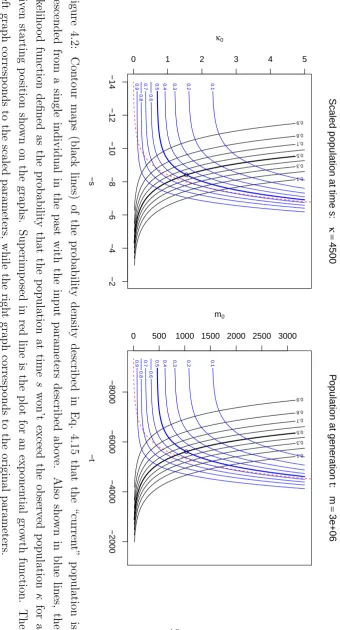
200,000 years ago. We define the “current” time to be the end of the upper pale-olithic period, which is around 10,000 BC. The reason is because, after that time, the growth rate λ increased dramatically following the invention of agriculture, whereasλ was (very approximately) constant for the≈150,000 years during the upper paleolithic period (Biraben, 1979). Goldewijk et al. (2010) estimates the size of the human population around the time to be around 1 million to 20 million. Thus, for the sake of the simulation, we will set M(t) = 3×106 _{to be the female}

population at the end of the paleolithic. As estimated by Biraben (1979), the an-nual growth rate is 0.008% per generation. Assuming one generation takes around 20 years, this corresponds with the annual growth logλ= 0.0015. In addition, as argued in Burden and Simon (2016), we will be using σ2 _{= 2. These parameters}

correspond to a ‘current’ scaled population ofκ= 4500. Last thing, we will define the likelihood function defined as the probability that the population at time s

won’t exceed the observed population κ given as follows;

L(s, κ0|κ) =Prob (κ(s)≤κ|κ(0) =κ0)

=

Z κ/(κ0es)

0

fZtot(u|s, κ0)du. (4.17)

(26)

Scaled population at time s: κ = 4500 −s κ0 0.1 0.3 0.5 0.7 0.8 0.9 −14 −12 −10 −8 −6 −4 −2

0 1 2 3 4 5

0.1 0.2 0.3 0.4 0.5 0.6 0.7 0.8 0.9 ● P

opulation at gener

ation t: m = 3e+06 −t m0 0.1 0.3 0.5 0.7 0.8 0.9 −8000 −6000 −4000 −2000

0 500 1000 1500 2000 2500 3000

[image:26.595.144.485.115.746.2]

(27)

4.2 The Coalescent Time of Two Individuals with

Wright-Fisher Model Imposed

In the previous section, the main assumption is the population grows stochas-tically as time progresses, hence it follows directly as a G-W process. Here, we assume that the the population size grows deterministically with varianceσ2 _{= 1,}

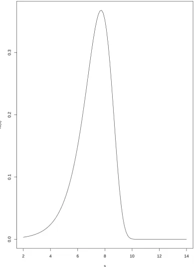
which corresponds with the W-F model. In the section, we will discuss the result from Slatkin and Hudson (1991) to find the the coalescent time i.e the time to the MRCA of a sample of two individuals at ”current” time with W-F model imposed. From page 558 of Slatkin and Hudson (1991), the probability density function for the coalescent time of two individuals (written in this thesis’ notations) is given by (See fig.4.3);

fS(s) =

2es

κ exp

2 (1−es₎

κ

(4.18)

with the mean coalescent time given as follows;

E(S) =

Z ∞

0

2ses

κ exp

2(1−es₎

κ

ds

u=es and du=esds

=

Z ∞

1

2ln(u)

κ exp

2(1−u)

κ

du

=2e 2

κ

Z ∞

1

ln(u) exp

₋

2u κ

du

=2e 2 κ κ Z ∞ 1 κ 2

e−κ2u

u du

=eκ2

Z ∞

1

e−κ2u

u du

t = 2u

κ and du= κ

2dt =

u tdt

=eκ2

Z ∞ 2

κ e−t

t dt

=eκ2E 1 2 κ , (4.19)

where E1(z) =

R∞ z

e−t

t dt is the exponential integral as defined in Abramowitz

and Stegun (1964) chapter 5. Slatkin and Hudson (1991) notes that for α 1 we have E1 _κ2

(28)

approximated to be around 0.577. Therefore, from Eq. (4.19) we have the mean coalescent time of the a sample of size two,

E(S) = e2κ

lnκ 2

−γ, (4.20)

(29)

2 4 6 8 10 12 14

0.0

0.1

0.2

0.3

s

[image:29.595.121.511.157.693.2]

fs(s)

(30)

Chapter 5 Novel Results and Discussion

We will derive new results in this chapter by formulating the density function of the MRCA of a sample of two randomly chosen individuals using a G-W process, and later generalize for the case of any sample size. Then, we will find their mean coalescent time and estimated population size at the time of the MRCA.

5.1 The Most Recent Common Ancestor of a

Sample of Two Individuals in a Galton-Watson

Process

In the previous section, Burden and Simon (2016) discussed the common ances-tor of the entire population at the current time. Here we are interested in the following question: Suppose we pick two random individuals from the current population, how long do we need to trace back in time until we find the common ancestor of these two individuals ?. Under G-W process and the same parameters used as before, we will start examining this case by first defining an event;

E2 = Event that two randomly chosen individuals at the “current” time s

are descended from a common ancestor at time 0.

(5.1)

Recall that we have previously defined the scaled population size as K(s) =

2M(τ) logλ

σ2 . Then, if we divide the current population as two sub-populations, say K1 = xK and K2 = (1 −x)K where K1 are the direct descendants from

(31)

function of K1 and K2 given that we have an initial population size κ0 and an

initial fraction of population _m1

0 whose descendants constitute a fractionx of the current population and an initial fraction 1− 1

m0 whose descendants constitute a fraction 1 − x of the current population. Denote this density function by

fK1,K2(κ1, κ2|s, κ0, m0). By the independence of parallel G-W processes, we then have;

fK1,K2(κ1, κ2|s, κ0, m0)dκ1dκ2 =fK1 κ1

s, κ0,

1

m0

!

dκ1fK2 κ2

s, κ0,1−

1

m0

!

dκ2

=fK xκ

s, κ0,

1

m0

!

dκ1

×fK (1−x)κ

s, κ0,1−

1

m0

!

dκ2, (5.2)

where the densityfK will be defined below by Eq. (5.5). From Eq. (4.7), we know

that Z and K are related via

Z = K(s)

κ0es

. (5.3)

Using Eq. (5.3) we can rewrite the solution to Forward-Kolmogorov equation in terms of K;

fK(κ|s, κ0, x0) = fZ

κ κ0es

s, κ0, x0

dz dκ

= 1

κ0es fZ

κ κ0es

s, κ0, x0

. (5.4)

Hence,

fK(κ|s, κ0, x0) =

1

es₋₁

x0κ0es κ

1₂

exp

 

−κ0

x0+_κκ₀e−s

1−e−s

 I1

  

2κ0

x0_κ₀κ_es

1₂

1−e−s   

+ 1

κ0es δ

κ κ0es

Π0(s, κ0, x0) (5.5)

where Π0(s, κ0, x0) is the probability that the fractionx0 of the initial population

eventually became extinct before time s with initial population κ0.

(32)

same thing to find the probability density that two randomly chosen individuals from population size K(s) are descended from a single individual at time s = 0 given we have the initial population size κ0 as follows ;

Prob (K(s)∈[κ, κ+dκ],E2|s, κ0)

=m0

Z 1

0

x2fX,K(x, κ|s, κ0)dxdκ. (5.6)

Note that m0 appears since we have m0 possibilities for the common ancestor of

the two individuals, andx2 _{appears since both individuals come from a fraction}_x

of the current total population size. In order to get the joint probability density function in X and K, we can apply the following using Jacobian transformation.

fX,K(x, κ|s, κ0) =fK1,K2(κ1, κ2|s, κ0, m0)

∂(κ1, κ2) ∂(x, κ)

=fK1,K2(κ1, κ2|s, κ0, m0)κ =κfK

xκ

s, κ0,

1

m0

fK

(1−x)κ

s, κ0,1−

1

m0

. (5.7)

Substitute this back to Eq. (5.6) yields;

=m0κdκ

Z 1

0 x2fK

xκ

s, κ0,

1

m0

fK

(1−x)κ

s, κ0,1−

1

m0

dx (5.8)

where, from Eq. (5.5),

fK xκ

s, κ0,

1

m0

= 1

es₋₁

κ0es m0xκ

1₂

exp

−κ0

m0 −xκe

−s

1−e−s ! I1    2κ0 xκ m0κ0es

1₂

1−e−s   

+δ(xκ) Π0

s, κ0,

1

m0

. (5.9)

Note that since m0 is arbitrarily large, it is very high in probability that the

fraction _m1

(33)

generations i.e. Π0

s, κ0,_m1₀

→1 as m0 → ∞. Therefore,

fK xκ

s, κ0,

1

m0

= 1

es₋₁

κ0es m0xκ

1₂

exp

−κ0

m0 −xκe

−s

1−e−s !

I1

  

2κ0

xκ m0κ0es

1₂

1−e−s  

+δ(xκ)

= 1

es₋₁

κ0es m0xκ

1₂

exp

−κ0

m0 −xκe

−s

1−e−s !

I1

  

2κ0

xκ m0κ0es

1₂

1−e−s   +

1

kδ(x)

(5.10)

But, by the property of delta function, we have R₀1x2δ(x)dx = 0. Hence, the contribution from the delta function in Eq. (5.10) is zero when being evaluated by Eq. (5.8). Therefore, we only have effectively

fK xκ

s, κ0,

1

m0

= 1

es₋₁

κ0es m0xκ

1₂

exp

−κ0

m0 −xκe

−s

1−e−s !

I1

  

2κ0

xκ m0κ0es

1₂

1−e−s   .

(5.11)

It is easily observed that κ0

xκ m₀κ₀es

1

2

1−e−s → 0 as 1

m0 → 0, hence by applying the property of modified Bessel function of first kind1,we can rewrite Eq. (5.11) as follows; fK xκ

s, κ0, 1 m0

= κ0

m0(es−1)(1−e−s)

exp

−κ0

m0 −xκe

−s

1−e−s !

= κ0

m0(es₋₁₎₍₁₋_e−s₎exp ₋

xκe−s

1−e−s +O 1 m2 0

as m0 → ∞. (5.12)

Similarly, applying the solution of Forward-Kolmogorov equation for the other

1_{That is}_I

1(2ω) =ω+O ω2

(34)

sub-population and collecting all the terms involving _m1

0 gives;

fK

(1−x)κ

s, κ0,1−

1

m0

= 1

es₋₁

κ0es− κ0e s

m0 (1−x)κ

!1₂

exp −κ0+

κ0

m0 −(1−x)κe

−s

1−e−s

! I1    2κ0

(m0−1)(1−x)κ m0κ0es

1₂

1−e−s

  +

1

κδ(1−x) Π0

s, κ0,1−

1

m0

= 1

es₋₁

κ0es

(1−x)κ

1₂

exp

₋

κ0−(1−x)κe−s

1−e−s

I1

  

2κ0

₍₁₋_x₎_κ κ0es

1₂

1−e−s   

+ 1

κδ(1−x) Π0(s, κ0,1) +O

1

m0

asm0 → ∞. (5.13)

We can ignore O_m1

0

terms as m0 → ∞. Note that in this case we need to

consider the extinction probability as 1− 1

m0 fraction of population in the past might have gone extinct with finite probability. Substitute these back to Eq. (5.8) yields;

=κdκ

Z 1 0

x2 κ0

(es₋₁₎₍₁₋_e−s₎exp ₋

xκe−s

1−e−s "

1

es₋₁

κ0es

(1−x)κ

1₂

exp

₋

κ0−(1−x)κe−s

1−e−s

I1

2κ0

1−e−s

(1−x)κ κ0es

1₂!

+ 1

κδ(1−x)Π0(s, κ0,1)

#

dx. (5.14)

Setting

g(x) = x

2_κ 0

(es₋_{1) (1}₋_e−s₎exp ₋

xκe−s

1−e−s

1

κΠ0(s, κ0,1) (5.15)

we can rewrite Eq. (5.14) as,

=κdκ

" Z 1

0

x2

(1−x)12

1

(es₋₁₎2₍₁₋_e−s₎

κ3 0es κ

12 exp

₋

κ0−κe−s

1−e−s

×I1

2κ0

1−e−s

(1−x)κ κ0es

1₂!

dx+

Z 1

0

g(x)δ(1−x)dx

#

(35)

Noting that R₀1g(x)δ(1−x_)d.x=g(1) we then have

= (κ

3 0esκ)

1 2

(es₋₁₎2₍₁₋_e−s₎exp ₋

κ0−κe−s

1−e−s

dκ

Z 1 0

x2

(1−x)12

I1

2κ0

1−e−s

(1−x)κ κ0es

1₂!

dx+ κ0

(es₋_{1) (1}₋_e−s₎exp

−κe−s

1−e−s

Π0(s, κ0,1)dκ.

(5.17)

Using the integral 2

Z 1

0

x2

(1−x)12

I1

c(1−x)12

dx= 16I2(c)−2c

2

c3 , (5.18)

where

c= 2κ0 1−e−s

κ κ0es

1₂

= 2 (κ0κe

s₎12

es₋₁ , (5.19)

we have

= (κ

3 0esκ)

1 2

(es₋₁₎2₍₁₋_e−s₎exp

−κ0−κe−s

1−e−s

16I2(c) (es₋₁₎_c3

dκ

= 16 (κ

3 0esκ)

1 2

(es₋₁₎2₍₁₋_e−s₎_c3I2

2 (κ0κes)

1 2

es₋₁ !

exp

−κ0+κe

−s

1−e−s

dκ.

(5.20)

By doing the algebra, it is clear that we have

16 (κ3₀esκ) 1 2 (1−e−s₎_c3 =

2

κ(e

s₋

1)2, (5.21)

giving Eq. (5.20) as

=2

κI2

2 (κ0κes)

1 2

es₋₁ !

exp

−κ0+κe

−s

1−e−s

dκ. (5.22)

(36)

Recall from Eq. (4.14) that Burden and Simon (2016) found that;

Prob (K(s)∈[κ, κ+dκ]|s, κ0) =

1

es₋₁

κ0es κ

1₂

exp

−κ0+κe

−s

1−e−s

I1

2 (κ0κes)

1 2

es₋₁ !

dκ. (5.23)

Hence, in a similar manner as in Eq. (4.15), the probability the two randomly chosen individuals at the ”current” time are descended from one individual at

s= 0 is;

Prob (E2|K(s) =κ, K(0) =κ0, s) =

Prob (K(s)∈[κ, κ+dκ]|s, κ0)

=

2

κI2

2(κ0κes) 1 2 es₋₁

1

es₋₁

κ0es κ

1₂

I1

2(κ0κes) 1 2 es₋₁

. (5.24)

Recall that we have previously definedω = (κ0κes) 1 2

es₋₁ , then we can write Eq. (5.24) as;

Prob (E2|K(s) = κ, K(0) =κ0, s) = 2

κI2(2ω)

1

κωI1(2ω)

= 2I2(2ω)

ωI1(2ω) .

(5.25)

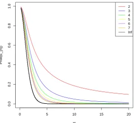
This probability is plotted in fig.5.1.

Next we will conduct an analytic check on Eq. (5.25) to see if the result is indeed a probability. We will check for both limiting cases i.e for ω → 0 and for

ω → ∞.

Check: Note that for ω → 0, we have I2(2ω) ≈ ω

2

2 and I1(2ω) ≈ ω(Abramowitz

and Stegun, 1964). Hence, substitute these back into Eq. (5.25) gives;

Prob (E2|κ(s) = κ, κ(0) =κ0, s)≈ ω2

(ω)(ω) = 1 as ω →0. (5.26) For ω→ ∞, we have;

I2(2ω)≈ e2ω

√

4πω

1− 1

ω +O

1

ω2

I1(2ω)≈ e2ω

√

4πω

1− 1

4ω +O

1

ω2

(37)

0 5 10 15 20

0.0

0.2

0.4

0.6

0.8

1.0

w

Prob(E_{n})

[image:37.595.174.448.138.388.2]

2 3 4 5 6 7 Inf

Figure 5.1: The plot of the probability thatnrandomly chosen individuals at time

shad a common ancestor at time 0 (See Eq. (5.25) forn= 2, and Eq. (5.39) for the general case) given that the current, scaled population size is K forn = 2,· · · ,7. The black curve is the limiting case as n → ∞ (See Eq. (4.15)). The parameter

ω is given by Eq. (4.16).

(Abramowitz and Stegun, 1964)

Substitute these back to Eq. (5.25) gives;

Prob (E2|κ(s) = κ, κ(0) =κ0, s)≈

2

ω

e2ω

√

4πω

1− 1

ω +O

1

ω2 e2ω

√

4πω

1− 1 4ω +O

1

ω2

≈0. (5.28)

From the checking, it can be seen that the probability defined in Eq. (5.25) has range between 0 and 1, hence it is indeed a probability.

The plot also tells us that when ω → 0 (corresponding to s → ∞), the probability that two individuals have a common ancestor at time 0 is almost certain because we have gone far enough back in time. On the other hand, when

(38)

5.2 The Most Recent Common Ancestor of a

Sample of n Individuals in a Galton-Watson

Process

In the previous section we discussed the case for sample of size two having a common ancestor in the past. The more interesting case is by choosing a sample of size n at present time and determine the likely parameters of their MRCA. This is what we will be trying to achieve in this section. In order to do get its probability density function, let’s define the following event;

En= Event that a random sample of size n of the “current”

population at times descended from a common ancestor at time 0. (5.29)

Again by dividing the current population size into two sub-populationsK1 taking

a fraction x of the current population, and K2 taking a fraction 1− x of the

current population, and following the similar procedure as with the case of two individuals, we can define the following;

Prob (K(s)∈[κ, κ+dκ],En|s, κ0)

=m0κdκ

Z 1

0 xnfK

xκ

s, κ0,

1

m0

fK

(1−x)κ

s, κ0,1−

1

m0

dx. (5.30)

Note that the term xn appears since n individuals come from the fraction x of the current population size. Using Eq. (5.12) and Eq. (5.13) for Eq. (5.30) gives;

=m0κdκ

Z 1

0 xn

κ0

m0(es−1)(1−e−s)

exp

₋

xκe−s

1−e−s       1

es₋₁

κ0es

(1−x)κ

1₂

exp

−κ0−(1−x)κe−s

1−e−s

I1

  

2κ0

(1−x)κ κ0es

1₂

1−e−s       + 1

κδ(1−x) Π0(s, κ0,1)

=κdκ " Z 1 0 xn

(1−x)12

1

(es₋₁₎2₍₁₋_e−s₎

κ3 0es κ

12 exp

₋

κ0−κe−s

1−e−s

×I1

2κ0

1−e−s

(1−x)κ κ0es

1₂!

dx

#

+

Z 1

0

(39)

where;

h(x) = x

n_κ

0

κ(es₋_{1) (1}₋_e−s₎exp

−xκe−s

1−e−s

Π0(s, κ0,1). (5.32)

Using the property of delta function, we have;

Z 1

0

h(x)δ(1−x)dx=h(1) = κ0

κ(es₋_{1) (1}₋_e−s₎exp ₋

κe−s

1−e−s

Π0(s, κ0,1).

(5.33)

Substitute back to Eq. (5.31) we have;

= (κ

3 0esκ)

1 2

(es₋₁₎2₍₁₋_e−s₎exp ₋

κ0−κe−s

1−e−s

dκ

Z 1

0

xn

(1−x)12

×I1

2κ0

1−e−s

(1−x)κ κ0es

1₂!

dx+ κ0

(es₋_{1) (1}₋_e−s₎exp ₋

κe−s

1−e−s

×Π0(s, κ0,1)dκ. (5.34)

Using the integral 3_,

Z 1

0

xn

(1−x)12

I1

c(1−x)12

dx= 2n+1c−n−1Γ(n+ 1)In(c)−

2

c. (5.35)

Setting

c= 2κ0 1−e−s

κ κ0es

1₂

= 2 (κ0κe

s₎12

es₋₁ (5.36)

and by definition;

Π0(s, κ0,1) = exp

₋

κ0

1−e−s

, (5.37)

(40)

then Eq. (5.34) can be written as ;

= (κ

3 0esκ)

1 2

(es₋_{1) (1}₋_e−s₎exp ₋

κ0−κe−s

1−e−s

×

"

2n+1_c−n_Γ(_n_{+ 1)}_I

n(c)−2

(es₋₁₎_c +

e−s

κ0κ

1₂#

dκ

= (κ

3 0esκ)

1 2

(es₋_{1) (1}₋_e−s₎exp

−κ0−κe−s

1−e−s

2n+1c−nΓ(n+ 1)In(c)

(es₋₁₎_c

dκ

=2

n+1_Γ(_n_{+ 1) (}_κ3 0esκ)

1 2 (es₋_{1) (1}₋_e−s₎ exp

−κ0−κe−s

1−e−s

In(c)

(es₋₁₎_cn+1

dκ

=2

n+1_Γ(_n_{+ 1) (}_κ3 0esκ)

1 2 (es₋₁₎2₍₁₋_e−s₎_cn+1 exp

₋

κ0−κe−s

1−e−s

In

2 (κ0κes)

1 2

es₋₁ !

dκ.

Noting that Γ(n+ 1) =n!, we then have;

= 2

n+1_n_{! (}_κ3 0esκ)

1 2

(es₋₁₎2₍₁₋_e−s₎_cn+1 exp

−κ0−κe−s

1−e−s

In

2 (κ0κes)

1 2

es₋₁ !

dκ

= n! (κ

3 0esκ)

1 2

(1−e−s_{) (}_κ

0κes)

1 2(n+1)

(es−1)n−1exp

−κ0+κe

−s

1−e−s

In

2 (κ0κes)

1 2

es₋₁ !

dκ

= n!κ

1−1 2n

0

(1−e−s_{) (}_κes₎n2

(es−1)n−1exp

−κ0+κe

−s

1−e−s

In

2 (κ0κes)12

es₋₁ !

dκ

= n!κ

1−1 2n

0 es

(es₋₁₎_κn2es 1 2n

(es−1)n−1exp

−κ0+κe

−s

1−e−s

In

2 (κ0κes)12

es₋₁ !

dκ

=n!κ

1−1 2n

0 e( 1−1

2n)s

κ12n

(es−1)n−2exp

−κ0+κe

−s

1−e−s

In

2 (κ0κes)12

es₋₁ !

dκ.

(5.38)

Using Eq. (5.23) again, the probability density that a random sample of size n

(41)

derived as follows;

Prob (En|s, κ0) =

Prob (K(s)∈[κ, κ+dκ]|s, κ0)

= n!κ (1−n

2)

0 e( 1−n

2)s(es−1)n−2

κn2−1ω

In(2ω)

I1(2ω)

= n!κ (1−n

2)

0 e( 1−n

2)s

κn2−1ω

(κκ0es) n

2−1

ωn−2

In(2ω)

I1(2ω)

= n!

ωn−1

In(2ω)

I1(2ω)

= n!

ωn−1

In(2ω)

I1(2ω). (5.39)

Lastly, as in the case of a sample of size two, we will also do the check to confirm that Eq. (5.39) is indeed a probability.

Check:

As ω → ∞, we have;

In(2ω)≈

e2ω

√

4πω

1− 4n

2₋₁

16ω +O

1

ω2

I1(2ω)≈ e

2ω

√

4πω

1− 3

16ω +O

1

ω2

. (5.40)

(Abramowitz and Stegun, 1964) Thus,

Prob (En|s, κ0)≈

n!

κ12n−1ωn−1 e2ω

√

4πω

1− 4n2₋₁

16ω +O

1

ω2 e2ω

√

4πω 1−

3 16ω +O

1

ω2

≈0, asω → ∞. (5.41)

As ω →0, we have;

In(2ω)≈

ωn n!

I1(2ω)≈ω. (5.42)

(Abramowitz and Stegun, 1964) Thus,

(42)

Scaled population at time s, kappa=4500

s κ0

0.1

0.2 0.3

0.4 0.5 _0.6

0.7 0.8 0.9

2 4 6 8 10 12 14

0

5

10

15

0.1

0.3 0.4 0.5 0.6 0.7 0.8 0.9

[image:42.595.150.471.138.425.2]

●

Figure 5.2: The black lines describe Eq. (5.39) that the n=2 randomly chosen individual at scaled time s are descended from a single ancestor in the past with scaled initial population κ0. Superimposed in blue are the likelihood function

that the “current” population won’t exceed the given population κ = 4500 as seen in Eq. (4.17). The red-dotted line is the exponential growth function for population.

Therefore, as seen above, for both limiting cases we have that Prob (En|s, κ0) ∈

[0,1], hence it is indeed a probability. Again, these two limiting cases tell us that when ω → ∞ (Corresponds to s → 0), the probability that a random sample of size n are descended from a common ancestor in the past is almost 0 because we have not gone back far enough in time. On the other hand, when ω → 0 (Corresponds to s→ ∞), it is very high in probability that a random sample of size nhave a common ancestor in the past because we have gone back far enough in time. Also, from fig.5.1, it can be seen there that Eq .(4.15) is the n → ∞

limit of Eq. (5.39)

(43)

(44)

5.3 The Mean Coalescent Time of Two

Ran-domly Chosen Individuals with a

Galton-Watson Process Imposed

In the previous sections we have derived the probability for both two and n

randomly chosen individuals having a common ancestor. Another interesting question is to estimate the expected time we need to trace back in time until we find the MRCA. As described in Section 4.2, this problem is related to the coales-cent. Slatkin and Hudson (1991) answered this question using the Wright-Fisher model; in our case we will assume a Galton-Watson. We will begin examining for the case of n randomly chosen individuals at time s, then specifically for the case of two randomly chosen individuals in order to be able to compare with the result found by Slatkin and Hudson (1991). Let’s define the following;

u(s, κ0) =Probability of having single ancestor at time zero from the sample of

size n taken from the current population at time s, given a starting

population κ0.

v(s, κ0) =Probability that the population at time s will not exceed the obeserved

current population given a starting populationκ0.

As defined in previous section, u(s, κ0) and v(s, κ0) have same definitions with

the following;

u(s, κ0) = Prob (En|K(0) =κ0, K(s) = κ)

v(s, κ0) = Prob (K(s)≤κ|K(0) =κ0). (5.44)

The functions u and v are both probabilities with u, v ∈ [0,1]. We will define corresponding continuous random variables U and V, and postulate a uniform prior distribution on these random variables, leading to the joint probability density

fU,V(u, v) = 1, 0≤u, v ≤1 (5.45)

In order to locate the MRCA in the (s, κ0)-plane, we need to apply a

transfor-mation using the Jacobian matrix to find the joint density function in terms ofs

and κ0, as follows,

fS,K0(s, κ0) = fU,V(u, v)

∂(u, v)

∂(s, κ0)

(45)

Recall that from Eq. (5.39) we have;

u(s, κ0) = n!

ωn−1

In(2ω)

I1(2ω)

where ω= (κκ0e

s₎12

es₋₁ . (5.47)

Note that ω as defined above can be written as follows;

ω = (κκ0e

s₎12

es₋₁ =

(κκ0)

1 2

es2 −e−

s

2

= (κκ0) 1 2

2 sinh s₂. (5.48)

Hence,

∂ω ∂s =−

(κκ0)

1

2 _cosh s

2

4sinh2 s₂ =− (κκ0)

1

2 _coth s

2

4sinh s

2

=−1

2ωcoth

s 2 (5.49) ∂ω ∂κ0 = 1 2κ 1 2κ−

1 2 0 2sinh s 2

4sinh2 s₂ =

κ12κ

−1 2

0

4sinh ₂s

= (κκ0) 1 2 2κ0 2sinh s₂

= ω

2κ0

(5.50)

Note: _dzd In(z)

zn

= In+1(z)

zn . Hence, forz = 2ω we have;

∂u ∂ω =n!

d dω

In(2ω)

ωn

ω I1(2ω)

= 2n−1n! d

dω

In(2ω) (2ω)n

I1(2ω)

2ω !

= 2nn!

"I1(2ω)

2ω

In+1(2ω)

(2ω)n −

In(2ω) (2ω)n

I2(2ω)

2ω

(I1(2ω)

2ω )2

#

= 2

n_n_!

(2ω)n−1

I1(2ω)In+1(2ω)−I2(2ω)In(2ω)

I1(2ω)2

= 2n!

ωn−1

I1(2ω)In+1(2ω)−I2(2ω)In(2ω)

I1(2ω)2

. (5.51) Thus, du dω =

2n!

(46)

where

Φ(ω) = I1(2ω)In+1(2ω)−I2(2ω)In(2ω)

I1(2ω)2

(5.53)

Using chain rule, we can find ∂u_∂s and _∂κ∂u

0 as follows;

∂u ∂s =

∂u ∂ω

∂ω ∂s =−

n!

ωn−2coth

s

2

Φ(ω) (5.54)

∂u ∂κ0 =

∂u ∂ω

∂ω ∂κ0 =

n!

κ0ωn−2Φ(ω). (5.55)

We now find a convenient representation of v(s, κ0) that will enable us to

calculate ∂v_∂s and _∂κ∂v 0.

Using Eq. (4.7) and Eq. (4.1), we have,

K(s) =κ0X(s). (5.56)

Then, Eq. (5.44) implies;

v(s, κ0) =L(s, κ0|κ)

=Prob (K(s)≤κ|K(0) =κ0)

=Prob

X(s)≤ κ

κ0|X(0) = 1

=1−

Z ∞

κ κ₀

fX(x|s, κ0)dx. (5.57)

In the last line of Eq. (5.57), using Eq. (3.14) with x0 = 1 and Eq. (4.1), the density function fX corresponding to the random variable X(s) is,

fX(x|s, κ0) = κ0 es₋₁

es

x

1₂

exp

₋

κ0(es+x) es₋₁

I1

"

2κ0(xes)

1 2

es₋₁ #

+δ(x) exp

−κ0

1−e−s

. (5.58)

Note thatfX(x|s, κ0) satisfies the Forward-Kolmogorov equation (See Eq. (3.13)), ∂fX(x|s, κ0)

∂s =−

∂

∂x(xfX(x|s, κ0)) +

1

κ0 ∂2

(47)

Using Eq. (5.59) we have;

∂v(s, κ0)

∂s =−

Z ∞

κ κ₀

− ∂

∂x(xfX(x|s, κ0)) +

1

κ0 ∂2

∂x2 (xfX(x|s, κ0))

dx = Z ∞ κ κ₀ ∂

∂x(xfX(x|s, κ0))−

1

κ0 ∂2

∂x2 (xfX(x|s, κ0))

dx

=

xfX(x|s, κ0)−

1

κ0 ∂

∂x(xfX(x|s, κ0))

∞

κ κ₀

=− κ−1

κ0 fX κ κ0

s, κ0

!

+ κ

κ2 0

∂ ∂xfX

κ κ0

s, κ0

!

. (5.60)

Since κ >0, theδ-function in Eq. (5.58) does not contribute, hence we have;

fX κ κ0

s, κ0

!

= κ0

es₋₁

esκ0 κ

1₂

exp

−κ+κ0e

s

es₋₁

I1(2ω). (5.61)

Taking the derivative of Eq. (5.58) with respect to x, and then setting x = _κκ 0 yields;

∂ ∂xfX

κ κ0

s,1, κ0

!

=− κ

5 2

0

2 (es₋₁₎2_κ32

es2e−

κ+κ0es es−1

h

−(κ0esκ)

1 2 _I

0(2ω)

+ (2κ+es)I1(2ω) +I1(−2ω)−(κκ0es)

1 2 _I

2(2ω)

i

(5.62)

Note that;

Iv(−z) = (−z)vz−vIv(z) (5.63)

(Abramowitz and Stegun, 1964)

therefore, for z = 2ω and v = 1 we have;

I1(−2ω) = −I1(2ω). (5.64)

Substitute this back to Eq. (5.62) we have;

∂ ∂xfx

κ κ0

s,1, κ0

!

=− κ

5 2

0

2 (es₋₁₎2_κ3₂e

s

2e−

κ+κ₀es es−1

h

−(κ0esκ)

1 2 _I

0(2ω)

+ (2κ+es)I1(2ω)−I1(2ω)−(κκ0es)

1 2 _I

2(2ω)

i

(48)

Substitute Eq. (5.61) and Eq. (5.65) into Eq. (5.60) gives us the explicit formula

∂v(s,κ0)

∂s as follows;

∂v(s, κ0)

∂s =−

κ−1

es₋₁

es_κ

0 κ

1₂

exp

−κ+κ0e

s

es₋₁

×I1(2ω) + κ0

2κ(es₋₁₎2 exp

−e

s_κ0 ₊_κ

es₋₁

×

"

κesI0(2ω)−

es_κ

κ0

1₂

(2κ+es−1)I1(2ω) +esκI2(2ω)

#

. (5.66)

Recall that we have;

fS,K0(s, κ0) = |JU,V(s, κ0)| (5.67)

where JU,V(s, κ0) is the Jacobian matrix.

Hence;

fS,K0(s, κ0) =

∂u ∂s

∂v ∂κ0

− ∂u

∂κ0 ∂v ∂s

. (5.68)

At this point, we have everything to evaluate Eq. (5.68), except _∂κ∂v

0. In order to find _∂κ∂v

0, we will do it numerically using a forward finite difference defined as follows;

∂v(s, κ0) ∂κ0

= L(s, κ0+|κ)−L(s, κ0|κ)

(5.69)

whereL(s, κ0|κ) is defined in Eq. (5.57). Substitute all of these back to Eq. (5.68)

and by using R program to plot the result, we get the following contour map for the joint probability of s and κ0 as shown in fig.5.3.

Finally, taking the integral over κ0 of fs,κ0(s, κ0) gives the marginal distribution

fS(s) as shown in fig.5.4. After finding the marginal distribution fs(s), we still

need to check that it is indeed a density function. In order to check, we take the integral overs offs. Using the current input parameters and R program, we get;

Z s

fs(s)ds≈0.9498109 (5.70)

Since it’s not exactly equal to 1 but close to 1, we need to make sure whether the cause is because of the rounding errors from using the Finite Difference for

∂v

(49)

Scaled population at time s: k=4500

s κ0

0.01 0.02

0.03

0.04

0.06

2 4 6 8 10 12 14

0

5

10

15

0.1

0.2 0.3

0.4

0.5 _0.6

0.7 0.8 0.9

0.1

0.3 0.4 0.5 0.6 0.7 0.8 0.9

[image:49.595.173.450.131.381.2]

●

Figure 5.3: The contour map for the joint density function of s and κ0 of two

randomly chosen samples (See Eq. (5.68)) withκ= 4500,σ2 _{= 2 and the growth}

rate log λ = 0.0015 given the initial population size of 3×106_{. Also, we used} = 10−9 _{for the finite difference. Superimposed in the contour is fig.5.2.}

for the scaled current population size κ= 3, taking the integration for this input gives a result which is very close to 1. Hence, we can be assured that it is most likely that for larger κ, we missed some part of the left tail of fig.5.4 (which do not behave properly for a very small value of s, but behaves properly if we use small value of κ) during the calculation. Thus, we can conclude that it is indeed a density function since the test with small value ofκ gives integral which is very close to 1 (around 0.99).

There is another way of finding fS without using finite difference for _∂κ∂v₀ as

given below;

Taking the integral of Eq. (5.68) overκ0 gives the marginal distribution function

with respect to the scaled continuous time steps given by;

fS(s) = Z ∞

0

∂u ∂s

∂v ∂κ0

− ∂u

∂κ0 ∂v ∂s

The Most Recent Common Ancestor of a Randomly Chosen Sample in a Galton Watson Process