HIGH PERFORMANCE INTEGRATION OF DATA PARALLEL FILE SYSTEMS AND COMPUTING: OPTIMIZING MAPREDUCE

(1)

HIGH PERFORMANCE INTEGRATION OF DATA PARALLEL FILE

SYSTEMS AND COMPUTING:

OPTIMIZING MAPREDUCE

Zhenhua Guo

Submitted to the faculty of the University Graduate School in partial fulfillment of the requirements

for the degree Doctor of Philosophy

in the Department of Computer Science Indiana University

(2)

Accepted by the Graduate Faculty, Indiana University, in partial fulfillment of the require-ments of the degree of Doctor of Philosophy.

Doctoral Committee

Geoffrey Fox, Ph.D. (Principal Advisor)

Judy Qiu, Ph.D.

Minaxi Gupta, Ph.D.

(3)

Copyright c

2012

Zhenhua Guo

(4)

(5)

Acknowledgements

First and foremost, I owe my sincerest gratitude to my advisor Prof. Geoffrey Fox. Throughout my Ph.D. research, he guided me into the research field of distributed systems; his insightful advice inspires me to identify the challenging research problems I am interested in; and his generous intelligence support is critical for me to tackle difficult research issues one after another. During the course of working with him, I learned how to become a professional researcher.

I would like to thank my entire research committee: Dr. Judy Qiu, Prof. Minaxi Gupta, and Prof. David Leake. I am greatly indebted to them for their professional guidance, generous support, and valuable suggestions that were given throughout this research work.

I am grateful to Dr. Judy Qiu for offering me the opportunities to participate into closely related projects. As a result, I obtained deeper understanding of related systems including Dryad and Twister, and could better position my research in the big picture of the whole research area.

I would like to thank Dr. Marlon Pierce for his guidance and support of my initial science gateway research. Although the topic of this dissertation is not science gateway, he helped me to strengthen my research capability and lay the foundation for my subsequent research on distributed systems. In addition, he provided excellent administrative support for the use of our laboratory clusters. Whenever I had problems with user accounts or environment setup, he was always willing to help.

(6)

Without the continuous support and encouragement from my family, I could not have come this far. Whenever I encountered any hurdle or frustration, they were always there with me. The love carried by the soothing phone calls from my parents was the strength and motivation for me to pursue my dream. Words cannot fully express my heartfelt gratitude and appreciation to my lovely wife Mo. She accompanied me closely through hardship and tough times in this six year long journey. She made every effort to help with my life as well as my research. They make the long Ph.D. journey a joyful and rewarding experience.

(7)

Abstract

The ongoing data deluge brings parallel and distributed computing into the new data-intensive computing era, where many assumptions made by prior research on grid and High-Performance Computing need to be reviewed to check their validity and explore their performance implication. Data parallel systems, which are different from traditional HPC architecture in that compute nodes and storage nodes are not separated, have been proposed and widely deployed in both industry and academia. Many research issues, which did not exist before or were not under serious consideration, arise in this new architecture and have drastic influence on performance and scalability. MapReduce has been introduced by the information retrieval community, and has quickly demonstrated its usefulness, scalability and applicability. Its adoption of data centered approach yields higher throughput for data-intensive applications.

(8)

List of Tables

1.1 map and reduce operations . . . 7

3.1 FutureGrid software stack . . . 36

3.2 FutureGrid clusters . . . 37

3.3 Specification of Bravo . . . 37

3.4 Job run time w/SandNvaried (fixed 400GB input) . . . 39

3.5 Job turnaround time w/SandDvaried . . . 40

3.6 IO performance of local disks . . . 46

3.7 IO performance of NFS . . . 46

3.8 IO performance of HDFS . . . 47

3.9 IO performance of Swift (single cluster) . . . 48

3.10 IO performance of Swift (cross-cluster) . . . 48

3.11 IO performance for small files . . . 49

4.1 Comparison of HDFS and Lustre . . . 55

4.2 Symbol definition . . . 58

4.3 Expand cost matrix to make it square . . . 63

4.4 Expand cost matrix to make it square . . . 66

4.5 System Configuration . . . 70

4.6 Examples of How Tradeoffs are Made . . . 80

5.1 Trade-off of task granularity . . . 86

5.2 Configuration of test environment . . . 103

6.1 Allocation policies of residual resources . . . 112

(14)

6.3 Energy consumption of regular and speculative tasks (Data Accessing) . . . 114

7.1 Symbols used in data partition formulation . . . 133

7.2 The fields and description of AutoDock MapReduce input . . . 134

7.3 The specification of cluster nodes . . . 135

(15)

List of Figures

1.1 Architecture of traditional High Performance Computing (HPC) systems . . . 4

1.2 Architecture of data parallel systems . . . 6

1.3 HDFS Architecture . . . 7

1.4 The breakdown of the execution of MapReduce applicationwordcount . . . 9

2.1 Taxonomy . . . 16

2.2 OpenMP stack . . . 18

2.3 OpenMP C program example . . . 19

2.4 Dryad ecosystem . . . 26

2.5 Sector system architecture . . . 27

2.6 Sawzall example . . . 30

2.7 HIVE system architecture . . . 31

3.1 Job run time with the number of nodes varied . . . 40

3.2 Job run time for different configurations . . . 42

3.3 Average run time of map tasks . . . 44

3.4 Average run time slowdown of map tasks . . . 45

4.1 Typical network topology . . . 52

4.2 The architecture of Lustre . . . 54

4.3 An example of MapReduce scheduling . . . 56

4.4 The deduction sketch for the relationship between system factors and data locality . . . 59

4.5 An example showing Hadoop scheduling is not optimal . . . 61

4.6 Algorithm skeleton of lsap-sched . . . 64

(16)

4.8 Single-cluster performance . . . 68

4.9 Cross-cluster performance . . . 69

4.10 Impact of various factors on the goodness of data locality and Comparison of real trace and simulation result . . . 73

4.11 Comparison of data locality (varied the num. of nodes) . . . 75

4.12 Comparison of data locality (varied rep. factor and the num. of tasks) . . . 75

4.13 Comparison of data locality cost (with equal net. bw.) . . . 76

4.14 Comparison of DLC with 50% idle slots . . . 77

4.15 Comparison of DLC with 20% idle slots . . . 78

4.16 Comparison of DLC w/ rep. factor varied . . . 78

4.17 Tradeoffs between fairness and data locality . . . 85

5.1 Examples of task splitting and task consolidation. Arrows are scheduling decisions. Each node has one map slot and blockBiis the input of taskTi . . . 91

5.2 Algorithm skeleton of Aggressive Split . . . 94

5.3 Different ways to split tasks (Processing time is the same). Dashed boxes represent newly spawned tasks. . . 96

5.4 Algorithm skeleton of Aggressive Split with Prior Knowledge . . . 97

5.5 Different ways to arrange the execution of a job . . . 102

5.6 Multiple scheduled jobs (Each uses all resources for execution) . . . 102

5.7 Single-Job test results (Gaussian distribution is used) . . . 105

5.8 Single-Job test results (Real profiled distribution is used) . . . 106

5.9 Multi-Job test results (task execution time is the same for a job) . . . 107

5.10 Multi-Job test results (job execution time is the same) . . . 107

6.1 Comparison of regular and speculative tasks . . . 116

6.2 An example of native Hadoop scheduling and resource stealing . . . 118

6.3 Results forts-map(‡NBST: Non-Beneficial Speculative Tasks) . . . 119

6.4 Results for PSA-SWG . . . 122

6.5 Results forts-mapwith straggler nodes. There are two straggler nodes for (a) and (b), and four straggler nodes for (c) and (d) . . . 123

6.6 Job run time for reduce-mostly applications . . . 125

6.7 Job run time for network-intensive applicationmr-wc . . . 126

(17)

7.1 Hierarchical MapReduce (HMR) architecture . . . 130

7.2 Hierarchical MapReduce (HMR) architecture with multiple global controllers . . . 132

7.3 Number of running map tasks for an Autodock MapReduce instance . . . 136

7.4 Number of map tasks executed on each node . . . 136

7.5 Execution time of tasks in different clusters . . . 137

7.6 Execution time of tasks in different clusters (even data distribution) . . . 139

7.7 The number of tasks and execution time in different clusters . . . 140

7.8 Hybrid MapReduce (HyMR) architecture . . . 142

(18)

List of Acronyms

OpenMP Open Multi-Processing MPI Message Passing Interface PVM Parallel Virtual Machine

PGAS Partitioning Global Address Space HPC High Performance Computing HTC High Throughput Computing MTC Many Task Computing HyMR Hybrid MapReduce HMR Hierarchical MapReduce DAG Directed Acyclic Graph

DAGMan Directed Acyclic Graph Manager

BOINC Berkeley Open Infrastructure for Network Computing GFS Google File System

HDFS Hadoop Distributed File System HiveQL Hive Query Language SQL Structured Query Language UDF User Defined Function

NUCC Non Uniform Cluster Computing

GALS Globally Asynchronous Locally Synchronous UDT UDP-based Data Transfer

SPE Sphere Processing Engine SJF Shortest Job First

BASE Benefit Aware Speculative Execution LSAP Linear Sum Assignment Problem BoT Bag-of-Tasks

(19)

UPC Unified Parallel C

SPMD Single Program Multiple Data GPFS General Purpose File System DPSS Distributed Parallel Storage Server SRB Storage Resource Broker

FTP File Transfer Protocol PVFS Parallel Virtual File System PBS Portable Batching System VM Virtual Machine

APU Atomic Processing Unit

LATE Longest Approximate Time to End POSIX Portable Operating System Interface HTTP Hypertext Transfer Protocol

IU Indiana University

XML Extensible Markup Language MDS Multidimensional Scaling

MI-MDS Majorizing Interpolation Multidimensional Scaling SWG Smith Waterman Gotoh

(20)

1 Introduction and Background

1.1 Introduction

After the eras of experimental, theoretical and computational science, we now enter the new era of data-intensive science. Tony Hey et al’s bookThe Four Paradigmdepicts the characteristics of real data-intensive applications from various fields including ocean science, ecological science and biology. The key character-istic is that scientists are overwhelmed with large data sets collected from many sources such as instruments, simulation, and sensor networks. Modern instruments such as Large Hadron Collider (LHC), next-generation gene sequencers and survey telescopes are collecting data in a unprecedented rate. For example, High Energy Physics (HEP) experiments produce tens of Petabytes of data annually, and Large Synoptic Survey Telescope produces data at a rate of 20 Terabytes per day.

The goal of e-Science is to transform raw data to knowledge, and advanced tools are necessary to accel-erate the time from data to insight. To process the ever-growing data requires large amounts of computing power and storage space, which far exceeds the processing capability of individual computers. Supercom-puters, clusters, clouds, and data centers have been built to facilitate science discovery. These systems adopt different architectures aligned with their specific design goals.

(21)

[image:21.612.203.444.290.446.2]

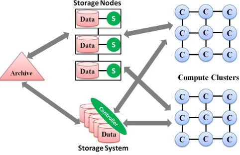
accelerate the communication among computers. In grid computing, clusters from multiple domains are fed-erated to enlarge available resource sets. These systems took a compute centered approach where compute nodes and storage systems are separated. As a result, parallel applications need to stage in data from storage nodes to compute nodes and store final results back to storage nodes (shown in Figure 1.1). In other words, its scheduling mechanism is bringing data to compute. Data grids were proposed to address the issue of how to manage large volumes of data across multiple sites. They adopt a hierarchical architecture in which par-ticipant sites are usually under the control of different domains and each site manages a portion of the whole data set. Still data and compute are not closely integrated.

Figure 1.1: Architecture of traditional HPC systems

Data-intensive applications operate on large volume of data. The progress of network and storage tech-nologies cannot keep pace with the rate of data growth, which is already a critical problem. Compute centered approach is not efficient because the cost to bring data to compute becomes significant and data transfer time may dominate the total execution time. For example, in grid the interconnection links between storage nodes and compute nodes are oversubscribed at a high ratio. That implies that the aggregate bandwidth of all nodes is way higher than the capacity of the interconnection links connecting storage and compute nodes. So only a few compute nodes/cores can concurrently fetch data from storage nodes at full speed. As a result, the in-terconnection links become bottleneck for data intensive applications. This fact renders it inefficient to move input data around.

(22)

systems have been developed among which MapReduce [54] and Dryad [73] are the most prominent tech-nologies. These systems take adata centeredapproach where data affinity is explicitly supported (e.g. local data accesses are favored over cross-rack data fetch). These systems can run some massively parallel infor-mation retrieval and web data processing applications on thousands of commodity machines, and achieve high throughput. Dryad was developed by Microsoft. But in late 2011, Microsoft dropped Dryad [9] and moved on to MapReduce/Hadoop.

1.2 Data Parallel Systems

Data parallel systems, which are natively designed for data-intensive applications, have been adopted widely in industry. The architecture is shown in Figure 1.2. The typical systems are GFS [62]/MapReduce[54], Cosmos/Dryad [73], and Sector/Sphere [65]. In these systems, the same set of nodes is used for both compute and storage. So each node is responsible for both computation and storage. This brings more scheduling flex-ibility to exploit data locality compared with the traditional architecture. For instance, the scheduler can bring compute to data, bring compute close to data, or bring data to compute. Ideally, most of data staging network traffic should be confined to the same rack/chassis to minimize cross-rack traffic. Traditionally, parallel file systems make data access transparent to user applications by hiding the underlying details of data storage and movement. For data parallel systems, this is insufficient as the runtime needs to know more information to make data location aware scheduling decisions. Thus location information of data is exposed to distributed runtimes.

1.2.1 Google File System (GFS)

(23)

[image:23.612.198.454.121.337.2]

Figure 1.2: Architecture of data parallel systems

Fig. 1.3 shows the architecture of HDFS. A centralnamenodemaintains the metadata of the file system. Its main responsibilities include block management and replication management. Real data are stored on

datanodesmanaged by thenamenode. HDFS allows administrators to specify network topology and thus is rack-aware. Metadata requests from HDFS clients are processed bynamenode, after which clients directly communicate withdatanodesto read and write data. Thenamenodeis a single point of failure because all metadata are lost if it fails permanently. To mitigate the problem, a secondarynamenoderuns simultaneously which performs periodic checkpoints of the image and edit log of thenamenode.

1.2.2 MapReduce

MapReduce is a programming model and an associated implementation for processing large data sets.

1.2.2.1 MapReduce model

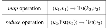
In MapReduce, input data are organized as key-value pairs. MapReduce supports two primitive operations:

mapandreduce(shown in Table 1.1), which was inspired by Lisp and other functional languages. Eachmap

(24)

[image:24.612.230.417.483.532.2]

Figure 1.3: HDFS Architecture

* Copied from http://hadoop.apache.org/common/docs/current/hdfs design.html

operation processes intermediate key-value pairs sharing the same key and generates final output. Because the intermediate data produced bymapoperations may be too large to fit in memory, they are supplied toreduce

operations via an iterator. It is users’ responsibility to implement map and reduce operations. Although this model looks simple, it turns out many applications can be expressed easily such as distributed grep, reversing web-link graph, distributed sorting and inverted indexing.

mapoperation (k1,v1)→list(k2,v2)

reduceoperation (k2,list(v2))→list(v3)

Table 1.1: map and reduce operations

1.2.2.2 MapReduce runtime

(25)

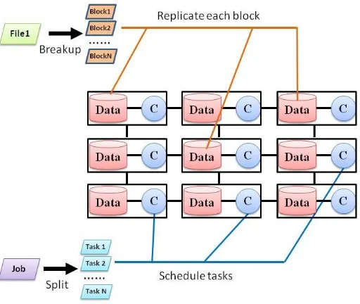
Primitivemapandreduceoperations are organized into schedulable map and reduce tasks. Each MapRe-duce job is comprised of some number of map and reMapRe-duce tasks. By default each map task processes the data of one block. Each slave node has a configurable number of map and reduce slots, which limit the maximum number of map and reduce tasks that can concurrently run on the node. When a task starts to execute, it occu-piesone slot; and when it completes, the slot isreleasedso that other tasks can use it. Conceptually, each slot can only have one task assigned at most at any time. There is a master node whereJob Trackerruns. The Job Tracker manages all slave nodes and runs a scheduler that assigns tasks to idle slots. When a slave node sends a heartbeat message and says it has available map slots, the master node first tries to find a map task whose input data are stored on that slave node. This is made possible because data location information is exposed by the underlying storage system GFS/HDFS. If such a task can be found, it is scheduled to the node and node-level data locality is achieved. Otherwise, Hadoop tries to find a task for rack-level data locality where input data and execution are on the same rack. If it still fails, Hadoop randomly picks a task to dispatch to the node. The default Hadoop scheduling policy is optimized for data locality.

To sum up, MapReduce integrates data affinity to facilitate data locality aware scheduling. It considers different levels of data locality, such as node level, rack level and data center level. Node level data locality means a task and its input data are co-located on the same node. Rack level data locality means a task and its input data are on different nodes that are located on the same rack.

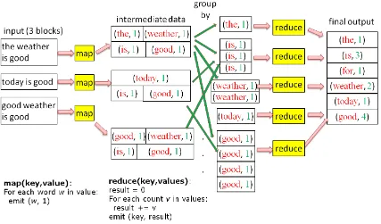
Fig. 1.4 shows the execution breakdown of MapReduce applicationwordcountwhich counts the number of occurrences of each word. The input text is split into three blocks. The implementations of map and reduce operations are shown near bottom left corner. Each block is fed into the map operation which tokenizes the text and emits value 1 for each encountered word. After all map tasks complete, the intermediate data are grouped by key and shuffled to the corresponding reduce tasks. Apartitioneris used to compute the mapping from intermediate keys to reduce tasks. After a reduce task collects all its input data, the reduce operation is applied which adds up the intermediate values and produces the final word count.

1.3 Motivation

(26)

[image:26.612.113.540.128.379.2]

Figure 1.4: The breakdown of the execution of MapReduce applicationwordcount

(27)

1.4 Problem Definition

Data parallel systems have been used to tackle large scale data processing and shown promising results for data-intensive applications. However, we observed the following issues in MapReduce model and runtimes which we strive to solve in this thesis.

• The performance of underlying storage systems has direct impact on the execution of upper-level par-allel applications. A detailed performance evaluation of Hadoop and contemporary storage systems has not been conducted. We hope to reveal their performance advantages/disadvantages and show how efficient they are.

• Hadoop assumes the work done by each task in a parallel job is similar to simplify implementation. However, this assumption does not always hold and thus severe load unbalancing can occur if tasks are intrinsically heterogeneous. We intend to figure out the ways to adjust tasks so that they are well balanced and thus job turnaround time is reduced.

• From our preliminary research, we have identified that in Hadoop resource utilization is constrained by the relationship between the numbers of task slots and tasks. By incorporating prior research from the HPC community, we wish to address the challenge of maximizing the efficiency of resource usage without interfering with native Hadoop scheduling.

• As we have shown, in data-intensive computing to move data around is not feasible and data locality becomes critical. The important of data locality has drawn attention in not only the MapReduce com-munity but also traditional grid computing communities. Current implementations use data-locality favored heuristics to schedule tasks. However, data locality itself has not been carefully analyzed the-oretically. We intend to quantify the importance of data locality and figure out the (sub-)optimality of state-of-the-art MapReduce scheduling algorithms.

(28)

complex problem which consists of both MapReduce algorithms and iterative MapReduce algorithms, the user needs to manually interact with different runtimes (e.g. Hadoop, Twister) to run individual jobs. A framework that seamlessly integrates and manages runtimes of different types is desired.

1.5 Contributions

We summarize the contributions of our research:

• A detailed performance analysis of widely used runtimes and storage systems is presented to reveal both the speedup and overhead they bring. Surprisingly, the performance of some well-known storage systems degrades significantly compared with native local I/O subsystems.

• For MapReduce, a mathematical model is formally built with reasonable data placement assumptions. Under the formulation, we deduce the relationship between influential system factors and data locality, so that users can predict the expected data locality.

• The sub-optimality of default Hadoop scheduler is revealed and an optimal algorithm based on Linear Sum Assignment Problem (LSAP) is proposed.

• Based on existing Bag-of-Tasks (BoT) model, a new task model Bag-of-Divisible-Tasks (BoDT) is proposed. Upon BoDT, new mechanisms are proposed that improve load balancing by adjusting task granularity dynamically and adaptively. Given BoDT model, we demonstrate that Shortest Job First (SJF) strategy achieves optimal average job turnaround time with the assumption that work is arbitrarily divisible.

• We propose Resource Stealing to maximize resource utilization, and Benefit Aware Speculative Ex-ecution (BASE) to eliminate the launches of non beneficial speculative tasks and thus improve the efficiency of resource usage.

(29)

1.6 Dissertation Outline

We present the state-of-the-art parallel programming models, languages and runtimes in chapter 2. What we have surveyed ranges from traditional HPC frameworks to recent data parallel frameworks, from low-level primitive programming support to high-level sophisticated abstraction, from shared-memory architecture to distributed-memory architecture. We focus on the level of abstraction, the target parallel architecture, large-data computation, and fault tolerance. By comparison, we demonstrate the advantage of large-data parallel systems over HPC systems for data-intensive applications, for which “move compute to data” is more appropriate than “move data to compute”.

In chapter 3, we evaluate the performance of Hadoop and some storage systems by conducting extensive experiments. We show how important system configurations such as data size, cluster size and per-node concurrency impact the performance and parallel efficiency. This performance evaluation can give us some insights about the current state of data parallel systems. In addition, the performance of local file system, NFS, HDFS and Swift are evaluated and compared.

In following chapters, we use MapReduce/Hadoop as the target research platform. The integration of data locality into task scheduling is a significant advantage of MapReduce. In chapter 4, we investigate the impact of various system factors on data locality. Besides, the non-optimality of default Hadoop scheduling is illustrated and an optimal scheduling algorithm is proposed. We conclude that our algorithm can improve performance significantly. Besides, we evaluate the importance of data locality for different cluster envi-ronments (single-cluster, cross-cluster, and HPC-style setup with heterogeneous network) by measuring how data locality impacts job execution time.

Hadoop is not efficient to run jobs with heterogeneous tasks. In chapter 5, the drawbacks of fixed task granularity in Hadoop are analyzed. Task consolidation and splitting are proposed which dynamically balance different tasks for the scenarios where prior knowledge is either known or unknown. In addition, for multi-job scenarios, we prove that Shortest Job First (SJF) strategy yields optimal average job turnaround time.

(30)

where resource stealing and Benefit Aware Speculative Execution (BASE) are proposed.

In chapter 7, Hierarchical MapReduce (HMR) and Hybrid MapReduce (HyMR) are proposed which expand the environments where MapReduce can be used and enable the simultaneous use of regular and iterative MapReduce runtimes respectively.

(31)

2 Parallel Programming Models and Distributed

Computing Runtimes

To fully utilize the parallel processing power of a cluster of machines, two critical steps are required. Firstly, domain-specific problems need to be parallelized and converted to the programming model program-mers choose. The chosen programming model should match the structure of the original problem naturally. Secondly, a distributed computing runtime is critical to manage highly distributed resources and run parallel programs efficiently.

Parallel computing models and languages relieve programmers from the details of synchronization, mul-tithreading, fault tolerance, etc. So programmers can focus on how to express their domain-specific problems in the chosen language or model. Each language or model has different tradeoffs among expressiveness, us-ability and efficiency. Many models have been proposed for shared-memory (e.g. OpenMP, multithreading), distributed shared-memory (e.g. PGAS) and distributed-memory platforms (e.g. MapReduce). Which model or language to choose depends on application characteristics (e.g. compute bound vs. IO bound, MapRe-duce vs. Directed Acyclic Graph (DAG)), system architecture (e.g. shared memory, distributed memory with low-latency network), and performance goal (e.g. latency vs. throughput).

(32)

Tasks in HPC jobs are tightly coupled. HPC is mainly designed for supercomputers and clusters with low-latency interconnects. Top500 [17] uses LINPACK as the benchmark to measure the performance of the fastest machines in the world which is expressed in flops per second. HTC emphasizes on executing as many tasks/jobs as possible for much longer time spans (e.g. months) and thus it prefers overall system throughput to the peak performance of an individual task. So HTC is measured by the number of tasks/jobs processed per month or per year. HTC can span over multiple clusters across different administrative domains by using various grid computing technologies. MTC lies between HPC and HTC, which emphasizes on utilizing as many resources as possible to accomplish a large number of computational tasks over short periods of time. Usually tasks in MTC are less coupled than those in HPC. In addition, MTC takes into consideration data-intensive computing where the volume of processed data may be extremely large.

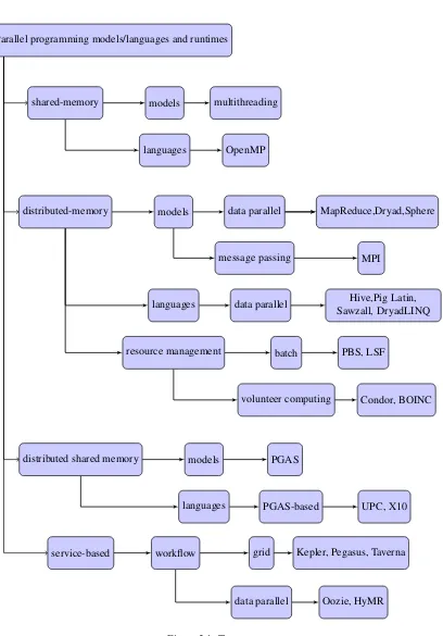
Below we survey the main programming languages, models and execution runtimes, the taxonomy of which is shown in Fig. 2.1.

2.1 Programming Models

For most non-trivial applications, sequential computation model quickly overwhelms the processing ca-pability of a single thread/process when the size of input data scales up. Parallelism of different types (e.g. task parallelism, data parallelism) can be exploited to accelerate task execution significantly. Several pro-gramming models have been proposed to unify the propro-gramming constructs or hide the complexity of man-aging underlying distributed resources. Overall they ease the development of parallel programs which run on multiple processor cores or multiple machines.

2.1.1 MultiThreading

(33)

Parallel programming models/languages and runtimes

shared-memory models multithreading

languages OpenMP

distributed-memory models data parallel MapReduce,Dryad,Sphere

message passing MPI

languages data parallel Hive,Pig Latin, Sawzall, DryadLINQ

resource management batch PBS, LSF

volunteer computing Condor, BOINC

distributed shared memory models PGAS

languages PGAS-based UPC, X10

service-based workflow grid Kepler, Pegasus, Taverna

[image:33.612.125.533.106.691.2]

data parallel Oozie, HyMR

(34)

much lower overhead than inter-process communication. The creation and termination of threads is faster than that of processes. Depending on implementation, threads are categorized into kernel threads and user threads. Kernel threads are managed by the kernel scheduler and thus can be scheduled independently. User threads are managed and scheduled in user space and the kernel is not aware of them. It is faster to create, manage and swap user threads than kernel threads. But multithreading is limited for user threads. When a user thread is blocked, the whole process is blocked as well and thus all other threads within the process get blocked even if some of them are ready to run.

For parallel programming, programmers need to explicitly control the synchronization among participant threads to protect the critical memory region accessed concurrently. The commonly used synchronization primitives include locks, mutexes, semaphores, conditional variables, etc.

Despite the conceptual simplicity, threading has several drawbacks. The isolation of thread execution is less rigid. The misbehavior of a thread can crash the whole process and thus result in the termination of the execution of all other threads belonging to the same process. In contrast, process-level isolation is more secure. In addition, multithreading only provides primitive building blocks which theoretically can be used to construct complicated applications. In practice, the complexity of writing and verifying thread-based parallel programs overwhelms the programmers even for modest-sized problems. Following is an excerpt from Lee’s paper.

“Although threads seem to be a small step from sequential computation, in fact, they represent a huge step. They discard the most essential and appealing properties of sequential computa-tion: understandability, predictability, and determinism. Threads, as a model of computation, are wildly nondeterministic, and the job of the programmer becomes one of pruning that nondeter-minism.” –The Problem with Threads, Edward A. Lee, UC Berkeley, 2006 [84]

2.1.2 Open Multi-Processing (OpenMP)

(35)

join back into the master thread, which continues to run until the end of the program. Threads communicate by sharing variables. Sometimes explicit synchronization is still needed to protect data conflicts and control race condition.

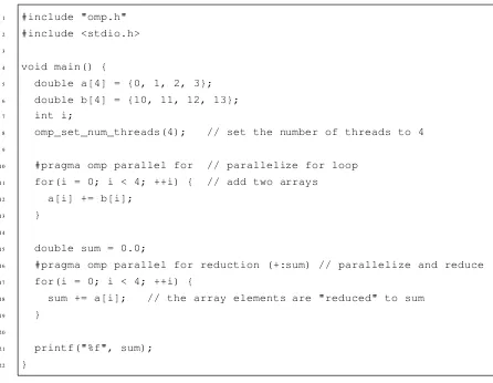
OpenMP supports C, C++ and Fortran. For each language, special compiler directives are defined to allow the users to explicitly mark the sections of code that can be run in paralle. Additional library routines are standardized from which each thread can get context information such as thread id.

Fig. 2.2 shows the solution stack of OpenMP. At the bottom is hardware which has multiple processors and maintains a shared address space. On top of it is the operating system with the support of shared mem-ory and multithreading. OpenMP runtime library utilizes the functionalities supported by OS and provides runtime support for upper level applications. Multiprocessing directives, OpenMP library and environment variables, which are the main building blocks to write parallel programs, are exposed to user applications.

Figure 2.2: OpenMP stack

* Copied from [5] Fig. 2.3 shows a simple OpenMP C example. Two arrays are declared and initialized in lines 5 and 6. The number of threads is set to 4 in line 8 whereomp set num threadsis a routine provided by OpenMP library. The directive in line 10 tells the compiler to parallelize the subsequent for loop which adds up arrays

(36)

1 #include "omp.h"

2 #include <stdio.h>

3

4 void main() {

5 double a[4] = {0, 1, 2, 3};

6 double b[4] = {10, 11, 12, 13};

7 int i;

8 omp_set_num_threads(4); // set the number of threads to 4

9

10 #pragma omp parallel for // parallelize for loop

11 for(i = 0; i < 4; ++i) { // add two arrays

12 a[i] += b[i];

13 }

14

15 double sum = 0.0;

16 #pragma omp parallel for reduction (+:sum) // parallelize and reduce

17 for(i = 0; i < 4; ++i) {

18 sum += a[i]; // the array elements are "reduced" to sum

19 }

20

21 printf("%f", sum);

[image:36.612.92.538.118.464.2]

22 }

Figure 2.3: OpenMP C program example

2.1.3 Message Passing Interface (MPI)

Multithreading and OpenMP are designed mainly for shared memory platforms. MPI is a portable, ef-ficient, and flexible standard specifying the interfaces that can be used by message-passing programs on distributed memory platforms. MPI itself is not an implementation, but a vendor-independent specification about what functionalities a standard-compliant library and runtime should provide. MPI interfaces have been defined for languages C/C++ and Fortran. There are a variety of implementations available in public domain (e.g. OpenMPI [13], MPICH [10,11]). Usually a shared file system (e.g. General Purpose File System (GPFS)) is mounted to all compute nodes to facilitate data sharing.

(37)

each MPI program may concurrently run multiple processes. Each communication may involve all processes, or a portion of processes. MPI definescommunicatorsandgroupswhich define the communication context and are used to specify which processes may communicate with each other. The processes within a process group are ordered and each process is identified by its rank in the group assigned automatically by the MPI system during the initialization. The identifiers are used by application developers to specify the source and destination of messages. The pre-defined default communicator isMPI COMM WORLDwhich includes all processes. MPI-1 supports both point-to-point and collective communication. MPI guarantees messages do not overtake each other. Fairness of communication handling is not guaranteed in MPI, so it is the users’ responsibility to prevent starvation.

Point-to-Point communication routines: The basic support operations aresendandreceive. Different types of routines are provided including synchronous send, blocking send/receive, non-blocking send/ re-ceive, buffered send, combined send/receive and “ready” send. Blocking send calls do not return until the message data have been safely stored so that the sender is free to modify the send buffer. However, the mes-sages may have not been sent out. The usual way to implement it is to copy the data to a temporary system buffer and thus it incurs the additional overhead of memory-to-memory copying. Alternatively MPI imple-mentations may choose not to buffer messages for performance reasons. In this case, a send call does not return until the data have has been moved to the matching receiver. In other words, the sender and receiver may or may not be loosely coupled depending on implementations. Synchronous send calls do not return un-til a matching receiver is found and starts to receive the message. Blocking receive calls do not complete unun-til the message is received. A communication buffer should not be accessed or modified until the corresponding communication completes. To maximize performance, MPI provides nonblocking communication routines that can be used to make communication and computation overlap as much as possible. A nonblocking send call initiates the operation and returns before the message is copied out of the send buffer. The program can continue to run while the message is copied out of the send buffer simultaneous in background by MPI run-time. A nonblocking receive call initiates the operation and returns before a message is received and stored into the receive buffer.

(38)

gather-to-all,reduction,reduce-scatter,scan, etc. When reaching thebarriersynchronization point, each process blocks until all processes in the group reach the same point. Broadcastssend a message from a “root” process to all other processes in the same group.Scatterdistributes data from a single source process to each process in the group, and each process receives a portion of the data (i.e. the message is split inton

segments and thei-th segment is sent to thei-th process). Thegatheroperation allows a destination process to receive messages from all other processes in the group and store them in rank order.Gather-to-alldistributes the concatenation of the data across processes to all processes. Reduceapplies a reduction operation across all members of a group. In other words, it operates on a list of data elements stored in different processes and produces a single output stored in the specified process. One example is sum calculation across all data distributed across processes. Reduce-scatterapplies element-wise reduction on a vector and distributes the result across the processes.

Process Topologies: MPI allows programmers to create a virtual topology and map MPI processes to positions in the topology. Two types of topologies are supported - Catesian (grid) and Graph. MPI does not define how to map virtual topologies to the physical structure of the underlying parallel system. Process topologies are usually used for the purposes of convenience or efficiency. Domain-specific communication patterns can be expressed easily with process topologies and ease the application development. For most parallel systems, the communication cost is not constant for all pairs of nodes (e.g. some nodes are “closer” than others). Process topologies can help MPI runtime to optimize the mapping of processes to physical processors/cores based on the physical characteristics and structures.

MPI I/O:MPI I/O adds parallel I/O support to MPI. It provides a high-level interface to describe data partitioning and data transfers. It lets users read and write files in synchronous and asynchronous modes. Accesses to a file can be independent or collective. Collective accesses allow for read and write optimization on various levels. MPI data types are used to express the data layout in files and data partitioning among processes. There has been substantial research on how to improve the performance of parallel IO [119,83,

120,47,127].

(39)

recovery [69,70] but they have not been standardized. In addition, data affinity/locality is not incorporated, which makes it inappropriate to run massively parallel applications on commodity clusters.

2.1.4 Partitioning Global Address Space (PGAS)

In shared memory model, data sharing is easy because the same memory region can be made accessible to multiple processes. In contrast, distributed memory platforms involve more hassle when intermediate data need to be shared among multiple processes. Usually, the programmer needs to write code to explicitly move data around for sharing. PGAS adopts distributed shared memory model [129]. The whole memory address space is partitioned into two portions: shared area and private area. The shared area is a global memory address space which is directly accessible by any process and can be used to store globally shared data. On the implementation side, the shared area is partitioned and physically resides on multiple machines. It is the PGAS runtime that creates the “illusion” of shared memory on top of distributed memory architecture. Therefore, the performance of data accessing may vary depending on where the accessed data are stored physically. Each process has affinity with a portion of the shared area and PGAS can exploit the reference locality. Shared data objects are placed in memory based on affinity, Private area is local to the corresponding process and not accessible by other processes. So any process can access global memory while only the local process may reference private area.

2.1.4.1 Unified Parallel C (UPC)

(40)

2.1.5 MapReduce

MapReduce [54] was initially proposed by Google and has gained popularity quickly in both industry and academia. MapReduce and its storage system GFS have been discussed in detail in section 1.2.2 and 1.2.1. Upon MapReduce model, some enhancements such as Map-Reduce-Merge and MapReduce online have been proposed with more features that make MapReduce applicable to more types of applications.

2.1.6 Iterative MapReduce

A large collection of science applications is iterative in that each iteration processes the data produced in last iteration and generates intermediate data that will be used as input by the next iteration until the result converges. Two typical examples are K-means and Expectation Maximization (EM). Iterative MapReduce can be implemented by pipelining multiple separate MapReduce jobs. However, this approach has signif-icant drawbacks. Firstly, for a logically individual problem, it involves multiple jobs the number of which is determined by convergence condition, so the additional overhead of starting, scheduling, managing and terminating jobs is inevitably incurred. Secondly, the intermediate data are serialized into disks and deserial-ized back into memory across iterations, which results in substantial overhead of disk accesses that are much slower than memory accesses. Iterative MapReduce runtimes have been developed to mitigate the issues.

2.2 Batch Queuing Systems

(41)

In batch queuing systems, jobs are submitted by users to job queues each of which has an associated priority. Each job is specified in a job description language/script by which users can specify how many compute nodes are needed, how long they are needed, and the location of output/error files. Based on the running jobs and jobs in queue, batch queuing systems calculate the availability of resources and reserve the specified number of nodes for a period of time. Mostly, compute nodes share a mounted global file systems. Input data can be stored in the shared file system, or programmers need to write scripts to explicitly stage in data. Usually, the order of job execution is determined based on submission time, the priority of the submitter’s account, and resource use history. To strictly follow the rules may result in significant resource fragmentation. For example, in a system comprising 5 nodes, taskA is running and using 3 nodes while task B andC are in queue which require 5 nodes and 2 nodes respectively. Task A will run for 1 hour before completion and tasksBandC will run for 2 hours and 30 minutes respectively. Because taskBis placed in front of taskC, Cwill not run until Bstarts to run. However, task C can be scheduled to run immediately without impacting the execution of task Bat all (anyway task B can start only after task A

completes). Backfilling [92] allows small jobs to leapfrog the large waiting jobs in the front of the queue without incurring significant delay on other jobs when there are sufficient idle resources to run those small jobs.

2.3 Data Parallel Runtimes

(42)

2.3.1 Hadoop

Hadoop is an open source implementation of MapReduce developed under the umbrella of Apache Source Foundation. Hadoop community is developing MapReduce 2.0 which dramatically changes the architecture to i) separate resource management and task scheduling/management, ii) mitigate the performance bottleneck of a single master node.

Some higher level projects have been built on top of Haddop and add additional functionalities. For example, Apache Mahout implements many widely used data mining and machine learning algorithms in a parallel manner so that data of larger-scale can be processed efficiently. Hive is a data warehouse software that supports querying and managing large data sets. Queries are converted to MapReduce jobs which are run on Hadoop.

2.3.2 Iterative MapReduce Runtimes

Some frameworks and enhancements to MapReduce have been proposed for iterative MapReduce appli-cations. HaLoop [34] modifies Hadoop to provide various caching options and reuse the same set of tasks to process data across iterations (i.e. tasks are loop-aware). Twister [57] and Spark [134] reuse the same set of “persistent” tasks to process intermediate data across iterations. Significant performance improvement over MapReduce has been shown for these frameworks.

2.3.3 Cosmos/Dryad

(43)

simultaneously on multiple nodes or multiple cores on a single node. Difference types of communication channels are supported such as files, TCP pipes and shared-memory FIFOs. Dryad automatically monitors the whole system and recovers from computer or network failures. If a vertex fails, Dryad reruns the task on a different node. A version number is associated with each vertex execution to avoid conflicts. If the read of input data fails, Dryad reruns the corresponding upstream vertex to re-generate the data. In initial version, greedy scheduling was adopted by the job manager with the assumption that it is the only job running in the cluster. Dryad applies run-time optimization that dynamically refines the graph structure according to network topology and application workload. Dryad runs on top of Cosmos which is a distributed file system that facilitates sharing and managing distributed data sets across the whole cluster. Although Dryad provides more advanced features compared to MapReduce, its use in both industry and academia is really limited and thus its scalability and performance for running diverse parallel applications have not been demonstrated.

Fig. 2.4 shows the Dryad ecosystem. Many languages such as Nebula and DryadLINQ have been ex-tended to integrate the processing capability of underlying Dryad systems. Existing sequential programs can be easily modified to become parallel.

Figure 2.4: Dryad ecosystem

* Copied from http://research.microsoft.com/en-us/projects/dryad/

2.3.4 Sector and Sphere

(44)

them into multiple files of smaller size. Sector can manage data distributed across geographically scattered data centers. One assumption made by Sector is that nodes are interconnected with high-speed network links. Sector is network topology ware, which means network structure is considered when data are managed. Data in Sector are replicated and per-file replication factor can be specified by users. Sector allows users to specify where replicas are placed (e.g. on local rack, on a remote rack). Permanent file system metadata is not required. If file system metadata is corrupted, the metadata can be rebuilt from real data. Data transfer is done with a specific transport protocol called UDP-based Data Transfer (UDT) which provides reliability control and congestion control. UDT has been shown to be fast and firewall friendly, and used by both commercial companies and research projects. Fig. 2.5 shows the architecture of Sector. Sector adopts a master-slave architecture. The Security Server maintains user accounts, file access permission information and authorized slave nodes. The Master Server maintains file system metadata, monitors slave nodes and responds to users’ requests. Real data are stored on slave nodes.

Figure 2.5: Sector system architecture

(45)

2.4 Cycle Scavenging and Volunteer Computing

Besides the massive computing power provided by dedicated supercomputers and clusters, personal com-puters can also provide a large amount of aggregate processing capability and storage space. The utilization of most PCs is low because they are mainly used for simple daily non compute-intensive work (e.g. web surfing, email send/receive). In other words, they have a large number of spare resources if combined. To efficiently harvest those idle CPU cycles and spare storage capacity can provision resources to complex sci-ence applications without incurring significant additional cost. Such systems are categorized into Volunteer Computing where computing resources are donated by owners. Because the contributed resources are highly distributed, network connection among them is drastically heterogeneous and each machine may join or leave at any time. As a result, the applications suitable for volunteer computing i) should not be IO-intensive, ii) have no or little communication among tasks, iii) are flexible for job completion time.

2.4.1 Condor

(46)

to large data applications.

2.4.2 Berkeley Open Infrastructure for Network Computing (BOINC)

BOINC [2,27], founded by University of California Berkeley, is an open source volunteer computing middleware that harvests the unused CPU and GPU cycles. Several of BOINC-based projects have been created including SETI@home, Predictor@home, and Folding@home. The BOINC resource pool is shared by many projects, so there is always work to be done and thus the whole system is kept busy and fully utilized. Hundreds of thousands computers are contributed, which provides nearly three petaflops processing power. BOINC provides support for redundant computing to identify and reject erroneous results (e.g. caused by mal-functioning computers, or malicious users).

2.5 Parallel Programming Languages

High level programming languages with native support of parallel data processing can lower the entry barrier to parallel programming. Programmers can directly utilize the constructs provided by these languages to achieve various types of parallelism.

2.5.1 Sawzall

(47)

1 count: table sum of int;

2 sum: table sum of float;

3 ele: float = input;

4 emit count <- 1;

5 emit sum <- x;

6 emit mean <- sum / count;

Figure 2.6: Sawzall example

which Sawzall makes additional optimization (e.g. coalesce intermediate data). Sawzall is built upon existing Google infrastructure such as Google File System and MapReduce and has been used by Google to process their log files.

Fig. 2.6 shows a simple Sawzall example that calculates the mean of all the float-point numbers in input files. Lines 1-2 declare three aggregators which are marked explicitly by keywordtable. Their aggregator types are bothsumwhich adds up the values emitted to it. Each record in input is converted to typefloatand stored in the variableeledeclared in line 3. Theemitstatement in line 4 sends value 1 to the aggregatorcount

whenever a record is encountered. Theemitstatement in line 5 sends each data value to the aggregatorsum. So after all records are processed, variablecountstores the number of records and variablesumstores the sum of all records. The mean is calculated in line 6.

2.5.2 Hive

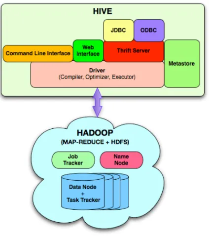
Hive [122,121] is an open source data warehousing platform built on top of Hadoop. It defines Hive Query Language (HiveQL) which is a Structured Query Language (SQL)-like declarative language. Hive adopts the well-understood concepts in databases such as tables, rows, columns and partitions. In additional, HiveQL allows users to plug their MapReduce programs into HiveQL queries so that complex logic can be directly expressed with MapReduce paradigm. The system architecture is shown in Fig. 2.7. HiveQL pro-grams are compiled into MapReduce jobs that run in Hadoop. Hive also provides a system catalogMetastore

(48)

[image:48.612.220.432.121.360.2]

Figure 2.7: HIVE system architecture

* Copied from [121]

2.5.3 Pig Latin

(49)

2.5.4 X10

X10 [40], a language developed by IBM, is designed specifically for parallel programming based on PGAS model. X10 is built on the foundation of Java, but overcomes its lack of lightweight and simple par-allel programming support. It is intended to increase programming productivity for Non Uniform Cluster Computing (NUCC) without sacrificing performance. Main design goals are safety, analyzability, scalability and flexibility. X10 is a type-safe object-oriented language with specific support of higher performance com-putation over dense and sparse distributed multi-dimensional arrays. X10 introduces dynamic, asynchronous activities as fundamental concurrency constructs, which can be created locally or remotely. Globally Asyn-chronous Locally SynAsyn-chronous (GALS) semantics is supported for reading and writing mutable data.

2.6 Workflow

2.6.1 Grid workflow

(50)

2.6.2 MapReduce workflow

(51)

3 Performance Evaluation of Data Parallel

Systems

In this chapter, we present the extensive experiments conducted to measure the efficiency of Hadoop and various storage systems including local IO subsystem, NFS, HDFS and Swift. The results obtained in this chapter will provide valuable insights for optimizing data parallel systems for data-intensive applications.

3.1 Swift

Swift is a new project under the umbrella of OpenStack. I would like to discuss its design specifically because it is more recent compared to other well-known systems to be evaluated. Swift is a highly available, distributed, eventually consistent object store. Swift is not a file system and typical Portable Operating System Interface (POSIX) semantics is not used. Swift clients interact with the server using HTTP protocol. Basic HTTP verbs such as PUT, GET and DELETE are used to manipulate data objects. The main components of Swift architecture are described below.

• Proxy Server: The Proxy Server is the gateway of the whole system. It responds to users’ requests

(52)

handoff server determined by the ring. All object reads/writes go through the proxy server which in turn interacts with internal object servers where data are physically stored.

• Object Server The Object Server is a object/blob storage server that supports storing, retrieval and deletion of objects. It requires file’s extended attributes (xattrs) to store metadata along with binary data. Each object store operation is timestamped and last write wins.

• Container ServerThe Container Server stores listings of objects calledcontainer. The Container Server does not store the location of objects. It only manages which objects are in each container. One good analogy is directories in local file systems.

• Account ServerThe Account Server manages listings of container servers.

• RingA ring represents a mapping from logical namespace to physical location. Given the name of an entity, its location can be found by looking up the corresponding ring. Separate rings are maintained for accounts, containers, and objects.

Swift supports large objects. A single uploaded object is limited to 5GB by default. Larger objects can be split into segments uploaded along with a special manifest file that records all the segments of a file. When downloaded, segments are concatenated and sent as a single object. In our Swift tests below, data size is way larger than 5GB and thus large object support is used.

Swift is designed for the scenarios where writes are heavy and repeated reads are rare. Since a Swift object server has so many files, the possibility of buffer cache hits becomes marginal. Based on these principles, to buffer disk data in memory does not benefit much. So in implementation, in-memory data cache is purged aggressively elaborated below.

• For write operations, cache is purged every time 512MB data are accumulated in cache.

• For read operations, cache is purged every time 1MB data are accumulated in cache

(53)

• For write operations, data are first written to memory, accumulated, and then flushed to disk later. So optimizations for bulk copy from memory to disk can be used.

• For read, each operation likely touches physical disks.

3.2 Testbeds

FutureGrid is an international testbed supporting new technologies at all levels of the software stack. The supported environments include cloud, grid and parallel computing (HPC). Table 3.1 summarizes the currently supported tools.

PaaS Hadoop, Twister, . . .

Iaas Nimbus, Eucalyptus, ViNE, OpenStack, . . . Grid Genesis II, Unicore, SAGA, . . . HPC MPI, OpenMP, ScaleMP, PAPI, . . .

Table 3.1: FutureGrid software stack

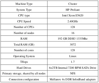
Our performance evaluation was carried out on FutureGrid clusters. Table 3.2 lists the basic specifica-tions of all FutureGrid clusters. Most of the experiments below were conducted in Bravo whose detailed specification is shown in Table 3.3. Unless stated specifically, Gigabit Ethernet is used.

3.3 Evaluation of Hadoop

Firstly, we evaluate the performance of Hadoop. Hadoop has many parameters that can be tuned. In our evaluation, three critical parameters are considered:

• the size of input (denoted byD)

• the number of nodes (denoted byN)

(54)

Name System Type # Nodes # CPUs # Cores TFlops RAM(GB) Storage(TB) Site

india IBM iDataPlex 128 256 1024 11 3072 335 IU

sierra IBM iDataPlex 84 168 672 7 2688 72 SDSC

hotel IBM iDataPlex 84 168 672 7 2016 120 UC

foxtrot IBM iDataPlex 32 64 256 3 768 0 UF

alamo Dell Power Edge 96 192 768 8 1152 30 TACC

xray Cray XT5m 1 168 672 6 1344 335 IU

[image:54.612.158.491.340.619.2]

bravo HP Proliant 16 32 128 1.7 3072 60 IU

Table 3.2: FutureGrid clusters

(copied from https://portal.futuregrid.org/manual/hardware)

Machine Type Cluster

System Type HP Proliant

CPU type Intel Xeon E5620

CPU Speed 2.40GHz

Number of CPUs 128

Number of nodes 16

RAM 192 GB DDR3 1333Mhz

Total RAM (GB) 3072

Number of cores 128

Operating System Linux

Tflops 1.7

Hard Drives 6x2TB Internal 7200 RPM SATA Drive Primary storage, shared by all nodes NFS

Connection configuration Mellanox 4x DDR InfiniBand adapters Table 3.3: Specification of Bravo

(55)

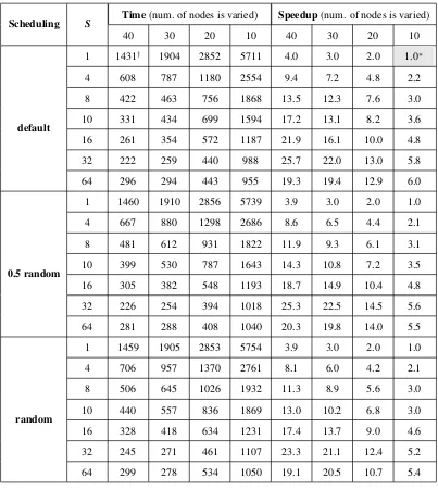
The first metric we choose is job turnaround timeTwhich is the wall-clock time between the time when a job is submitted and the time when it completes. However, absolute job turnaround time cannot reveal the efficiency of scaling out. When the number of nodes or map slots per node is increased, performance is expected to improve. Given a fixed amount of work to do, ideally the speedup ofTshould beS·Ncompared with the baseline configuration whereS andN are both 1. But the efficiency of scaling-out is much lower than the theoretical value in practice. For example, it is possible that job turnaround time is reduced by 2 times while number of nodes is increased by 10 times. So we normalize absolute job turnaround time to calculate parallel efficiency.

LetI1denote the normalized job turnaround time with respect to the number of nodes (i.e.I1is the time taken to process one unit of data using one node).I1can be calculated with (3.1).

T =I1·D

N ⇒ I1=

T·N

D (3.1)

We know that I1 = T ·N/D given a fixedS. Now we takeS into consideration. LetI2 denote the normalized job run time with respect to both the number of nodes and the number of slots per node. SoI2is the time taken to process one unit of data on one node by one map task. We assume all map slots are utilized during processing.I2can be calculated using (3.2).

I1= I2

S ⇒ I2=I1·S =

T·N·S

D (3.2)

In our tests, we varied the number of slave nodes between 10, 20, 30 and 40; varied the number of map slots per node between 1, 4, 8, 10, 16, 32 and 64; and varied the size of input data between 100GB, 200GB, 300GB and 400GB.

(56)

Scheduling S Time(num. of nodes is varied) Speedup(num. of nodes is varied)

40 30 20 10 40 30 20 10

default

1 1431† 1904 2852 5711 4.0 3.0 2.0 1.0∗

4 608 787 1180 2554 9.4 7.2 4.8 2.2

8 422 463 756 1868 13.5 12.3 7.6 3.0

10 331 434 699 1594 17.2 13.1 8.2 3.6

16 261 354 572 1187 21.9 16.1 10.0 4.8

32 222 259 440 988 25.7 22.0 13.0 5.8

64 296 294 443 955 19.3 19.4 12.9 6.0

0.5 random

1 1460 1910 2856 5739 3.9 3.0 2.0 1.0

4 667 880 1298 2686 8.6 6.5 4.4 2.1

8 481 612 931 1822 11.9 9.3 6.1 3.1

10 399 530 787 1643 14.3 10.8 7.2 3.5

16 305 382 548 1193 18.7 14.9 10.4 4.8

32 226 254 394 1018 25.3 22.5 14.5 5.6

64 281 288 408 1040 20.3 19.8 14.0 5.5

random

1 1459 1905 2853 5754 3.9 3.0 2.0 1.0

4 706 957 1370 2761 8.1 6.0 4.2 2.1

8 506 645 1026 1932 11.3 8.9 5.6 3.0

10 440 557 836 1869 13.0 10.2 6.8 3.0

16 328 418 634 1231 17.4 13.7 9.0 4.6

32 245 271 461 1107 23.3 21.1 12.4 5.2

[image:56.612.123.526.119.570.2]

64 299 278 534 1050 19.1 20.5 10.7 5.4

Table 3.4: Job run time w/SandNvaried (fixed 400GB input)

*: Baseline system configuration:S= 1,N= 10 †_{: Time is in second}

3.3.1 Job run time w.r.t the num. of nodes

We increased the number of nodes, and measured the job run time of different scheduling algorithms with

(57)

default 0.5 random random

S 400G† 100G‡ Slowdown∗ S 400G 100G Slowdown∗ S 400G 100G Slowdown∗

1 5711 1329 4.29 1 5739 1327 4.32 1 5754 1321 4.35

4 2554 538 4.74 4 2686 582 4.61 4 2761 625 4.41

8 1868 315 5.93 8 1822 404 4.50 8 1932 438 4.41

10 1594 277 5.75 10 1643 360 4.56 10 1869 370 5.05

16 1187 231 5.13 16 1193 248 4.81 16 1231 262 4.69

32 988 151 6.54 32 1018 207 4.91 32 1107 185 5.98

64 955 138 6.92 64 1040 111 9.36 64 1050 168 6.25

Table 3.5: Job turnaround time w/SandDvaried

†: time taken to process 400GB data (in seconds)

‡: time taken to process 100GB data (in seconds) * Given a fixedS, slowdown =time to process_{time to process}400₁₀₀GBdata_GBdata

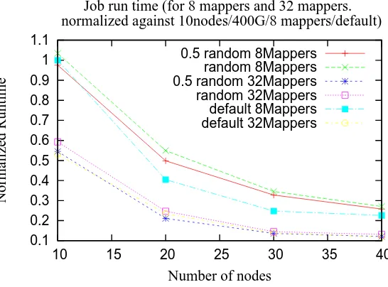
Sis 8,N is 10 and default scheduling is used.

0.1 0.2 0.3 0.4 0.5 0.6 0.7 0.8 0.9 1 1.1

10 15 20 25 30 35 40

Normalized Runtime

Number of nodes

Job run time (for 8 mappers and 32 mappers. normalized against 10nodes/400G/8 mappers/default)

[image:57.612.192.465.464.666.2]

0.5 random 8Mappers random 8Mappers 0.5 random 32Mappers random 32Mappers default 8Mappers default 32Mappers

(58)

• As we expect, the job run time is decreased as we increase number of nodes. But the relationship is not linear. The performance gain becomes less and less significant as we add more and more nodes. Even-tually, the reduction of job run time becomes marginal and using more resources gets cost prohibitive.

• Default scheduling has highest speedup. Random scheduling has lowest speedup. 0.5 random falls in between.

• Running 32 mappers per nodes yields much better performance than 8 mappers per node.

3.3.2 Job run time w.r.t the number of map slots per node

Theoretically, increasing S is a double-edged sword. On the one hand, it increases concurrency byP

times. On the other hand, it increases overhead byQtimes. P andQneed to be evaluated through experi-ments. The final outcome depends on the effects of above two factors. IfP > Q, it decreases job run time. IfP < Q, it increases job run time. Speedup isP/Q. Fig. 3.2 shows job run time withSvaried between 1, 4, 8, 10, 16, 32, and 64. We summarize our observations:

• The relationship is NOT linear. Ideally, job run time should be inversely proportional toS. But the plots show this is not the case.

• WhenSis small, increasingScan bring significant benefit so that job run time is decreased drastically. This is because increasingSalso improves concurrency so that the overlap between computation and IO, and the processing power of the multi-core processors can be better explored. The benefit of higher concurrency exceeds overhead.

• WhenSbecomes big (more than 32), job run time does not change much. For some tests, to increase

Sfrom 32 to 64 even results in the increase of job run time. This means the contention of resource use becomes comparable to the benefit of higher concurrency.

HIGH PERFORMANCE INTEGRATION OF DATA PARALLEL FILE SYSTEMS AND COMPUTING: OPTIMIZING MAPREDUCE