Localisation of Low Energy
Eigenfunctions to the Schr¨
odinger
Operator
Wenqi Zhang
October 2018
Declaration
The work in this thesis is my own except where otherwise stated.
Acknowledgements
This thesis would not have been possible without the patience and dedication of my supervisor Pierre Portal. His advice and enthusiasm has been paramount.
I would also like to thank (in no particular order) Ben Andrews, Bryan Wang, Jan Rozendaal, Neil Trudinger and Qi-Rui Li for their assistance at various times in the year with explaining difficult concepts.
Finally, discussions with Chris Williams have been valuable in better under-standing Brownian motion and fractal dimensions.
Abstract
We explore the phenomena where low energy eigenfunctions of the operator
L=−∆ +V for V ∈L∞ concentrate on a small subset of the original domain, and decay exponentially outside of this region. We consider the function usolving the equation Lu= 1 and show that 1
u acts as an effective potential, in the sense
that one can show
Z
|∇f|2+V f2 =
Z
u2|∇(f /u)|2+ 1
uf
2.
With this equality, it can be shown that the regions where 1u < λfor some (small) eigenvalue λ approximately corresponds to where the corresponding eigenfunction is localised.
Furthermore, if the regions where 1u < λare composed of suitably disjoint subsets, we show that if a (global) eigenfunction with eigenvalue λ resides in one of these subsets, then it is well approximated in this subset by local eigenfunctions (i.e. eigenfunctions of L in this subset) with eigenvalue λ±δ. For these subsets to exist, 1u needs to vary substantially. SinceusolvesLu= 1, this phenomena cannot occur when V is smooth, and does not vary substantially.
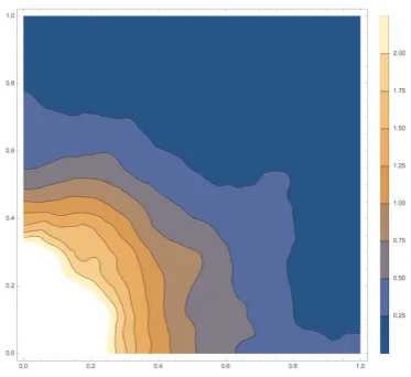
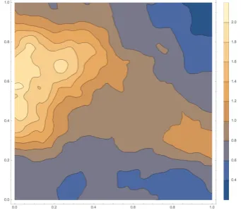
As a visual aid to gain intuition on how V affects the localisation, we simu-late the lowest energy eigenfunction to L numerically. We generate V to take random values on a dyadic grid. We vary the maximum size of the random values and the scale of the grid. Once the grid becomes sufficiently fine, and for large values of V we observe that the lowest energy eigenfunction become concentrated in one particular region. We conjecture that the maximum size ofV
has a greater effect on localisation than the grid size. This is also hinted at since the theorems depend only on ||V||∞. However, further work needs to be done for fractal potentialsV, in the sense that the set of discontinuities of our V may have the same Hausdorff dimension (no matter the grid size).
Finally, we also explore briefly the possibilities of defining a Brownian motion on Ω endowed with a distance associated with 1
u. The hope is to one day be able to
have a microscopic (Feyynman-Kac) description of the solution to ∂tu=Lu.We
Contents
Acknowledgements vii
Abstract ix
Notation and terminology xiii
1 Introduction and Preliminaries 1
1.1 Introduction . . . 1
1.2 Preliminaries . . . 4
1.2.1 Weak Formulation and Boundary Conditions . . . 6
1.2.2 Existence and Uniqueness of Solutions . . . 9
1.2.3 Regularity of Solutions . . . 11
1.2.4 Maximum Principle . . . 18
1.2.5 Spectral Decomposition. . . 20
2 Important Identities and Key Estimates 25 2.1 Important Identity . . . 25
2.2 Key Equalities . . . 26
3 Prelocalisation Estimates for the Agmon Distance 31 3.1 Agmon Distance . . . 31
3.2 Prelocalisation Estimates . . . 31
4 Localisation Estimates Using Landscape Function 41 4.1 Localisation of Eigenfunctions . . . 41
4.2 Numerical Simulation . . . 58
5 Further Research 63 5.1 Brownian Motion . . . 63
6 Appendix 69
6.1 Agmon’s Prelocalisation Estimates . . . 69
Notation and terminology
In the following Ω is an open subset of Rn
Notation
Rn+ the set{x= (x1, ..., xn)∈Rn :x1 ≥0} Ω+ = Ω∩Rn+
Cn(Ω) space of n times continuously differentiable functions on Ω, n≥0
Cn,α(Ω) space of n times differentiable functions on Ω, n ≥ 0 with α
H¨older continuous nth order derivatives.
C∞(Ω) =T
k≥0Ck(Ω)
Cc(Ω) space of continuous functions with compact support in Ω
Cc∞(Ω) =C∞(Ω)∩Cc(Ω)
Chapter 1
Introduction and Preliminaries
1.1
Introduction
Anderson localisation is a physical phenomena where the propagation of electrons becomes localised in disordered mediums [1]. Mathematically, this can be described as the low energy eigenfunctions of an elliptic operator concentrating (or localising) on a small portion of the original domain, and nearly zero on the remainder. Over the last half century, this phenomena has seen many applications in various fields such as condensed matter physics and engineering [1][2][3][4][5]. However, a mathematical treatment is lacking and to quote the 1977 Nobel lecture,
[localization] has yet to receive adequate mathematical treatment, and one has to resort to the indignity of numerical simulations to settle even the simplest questions about it.
−Philip W. Anderson, Nobel lecture, 8 December 1977.
In recent years the solutionuto Lu= 1 for an elliptic operatorL= −divA∇+V
for some suitable matrix A and potential V (commonly referred to as the land-scape function) has demonstrated remarkable accuracy in predicting the shape and location of localised low energy eigenfunctions [6]. It has been used in application successfully [7][8][9].
In 2018 a preprint containing the simplest mathematical treatment of the land-scape function to date was published on arXiv [10]. In this preprint the authors demonstrated that low energy eigenfunctions ofLreside in the wells of 1/uand de-cay exponentially across the barriers/extrema of 1/u. Furthermore, if the wells of 1/uare disjoint and suitably far apart, we observe that the eigenfunction localises
to one of these wells, and they are well approximated by local eigenfunctions (that is, eigenfunctions of Lwith the domain restricted to the well).
Perhaps the simplest case for which [10] applies to is the Schr¨odinger opera-tor,L= −∆ +V for some 0< V ∈L∞. Even in this case, localisation can still be observed for rough potentialsV, and many of the mathematical challenges simplify. Hence this thesis aims to present [10] in this simplified setting to emphasise the fundamental roleuplays in localisation. As we avoid many of the issues that [10] en-counter, we are able to present a self contained argument illustrating the key ideas.
We first demonstrate that the solutionutoLu= 1 is a unique, positive, continuous function, allowing us to safely write 1
u. Afterwards, we establish the fundamental
identity (Lemma 2.3), which states that for all f ∈W1,2(Ω) we have
Z
Ω
|∇f|2+V f2 =
Z
Ω
u2|∇(f /u)|2+ 1
uf
2.
Since u2|∇(f /u)|2 ≥0 we arrive at the inequality
Z
Ω
|∇f|2 +V f2 ≥
Z
Ω 1
uf
2
which can be seen as replacing V with 1u in the trivial inequality
Z
Ω
|∇f|2+V f2 ≥
Z
Ω
V f2.
Hence, the landscape function can be seen as an effective (quantum) potential, in the sense that we have replaced V with a function which combines the effects of both |∇f|2 (kinetic energy) and V f2 (potential energy) terms.
Without the landscape function, one can use the trivial inequality and [11] (Agmon’s method) to confine eigenfunctions with (low) eigenvalue λ to regions of the form {x:V(x)≤λ+δ}. This is, however useless in cases such as piecewise constant potentials with randomly generated constants [10].
With the inequality from the fundamental lemma, Agmon’s method can be used to instead confines the eigenfunction to a region of the form
E(λ+δ) :={x: 1
now since u is a continuous function, whereas V may not be, we can view 1/u as a continuous approximation ofV. In some sense it is more powerful than just any continuous approximation as it also contains information about the kinetic term. Furthermore these regions do approximate the location of the eigenfunction well, as demonstrated in application by [FM, A+2016, L+2016].
To formulate the above observations into precise theorems, we will consider the weight
ωλ(x) = max
1
u(x) −λ,0
.
with the associated Agmon metric given by
ρ(x, y) = inf
γ
Z
γ
1
ωλ(γ(t))1/2
|γ˙(t)|dt
where the infimum is taken over all absolutely continuous paths from x to y. Using the techniques of [11], presented by [10] we will develop prelocalisation estimates that show with respect to the Agmon metric, outside of the setsE(λ+δ) the eigenfunction (with eigenvalue λ) decays exponentially (Corollary 3.3). The existence of such a decomposition indicates that u cannot must vary substantially. This cannot occur when V is smooth, or has small oscillation.
We are primarily interested in the scenario when E(λ + δ) decomposes into a finite collection of disjoint subsets, with a large separation between the subsets. In this case, we can show that eigenfunctions are concentrated in one of these subsets, in the sense that they are well approximated by local eigenfunctions of L. This is the main result and is presented in Theorem 4.1.
After this result is established, we shift our focus and explore the possibility that the Agmon metric is a ‘natural’ metric for our operator L. We investigate the possibilities of defining a (reflected) Brownian motion on (Ω, ρ), inspired by [12]. We hope that in future, the heat kernel of exp(−∆ +V) can be recovered from this Brownian by the Feynman-Kac formula.
1.2
Preliminaries
We assume the reader is familiar with functional analysis and Hilbert space theory, for instance the Riesz-Fr´echet representation theorem (see [[14], Theorem 5.5, p. 135] for a reminder), the Hilbert space L2, the Stone-Weierstrass theorem, and Riesz-Markov-Kakutani representation theorem. We refer the reader to [14], [15], [16] if they need a reminder. We also assume a stronger version of Rademacher’s theorem, stated below
Theorem 1.1 If u is an absolutely continuous function then u is differentiable almost everywhere. In particular, if u is Lipschitz, then u is differentiable a.e.. This is proved in [[15], Theorem 3.11, p. 130].
We are be interested in the following class of functions.
Definition 1.2 Let Ω⊆Rn be an open set. The Sobolev space W1,2(Ω) is given by
u∈L2(Ω) :∃gi ∈L2(Ω) s.t.
Z
Ω
u∂ϕ ∂xi
=−
Z
Ω
giϕ ∀ϕ∈Cc∞(Ω), ∀i={1, ..., n}
.
We remark that this space is a Hilbert space with inner product
hu, viW1,2 :=hu, vi+
n
X
i=1
∂u ∂xi
∂v ∂xi
whereh·,·i is theL2 inner product. This result can be found in [[14], prop. 9.1, p.264] as well as [[17], Theorem 4.8, p. 41]. The associated norm is
kuk2W1,2 :=kuk 2 2+
n
X
i=1
k∂u ∂xi
k22
wherek·k2 denotes the L2 norm.
Another fact we need is the following denseness properties of W1,2(Ω).
Theorem 1.3 Let Ω ⊂ Rn be a bounded open set with continuous boundary.
Then
ˇ
C∞(Ω) :={u|Ω :u∈Cc∞(R n)}
See [[17], Theorem 7.7, p. 78] for a proof.
Since W1,2(Ω) is a Hilbert space, it is of interest to study its dual space. We use
W−1,2(Ω) to denote the dual space ofW1,2(Ω). However we do not use the Riesz-Fr´echet representation to identify W1,2(Ω) with W−1,2(Ω). Rather we identify (L2(Ω),h·,·i) to its dual,L2(Ω)?. This gives the relationship
W1,2(Ω)⊂L2(Ω)∼=L2(Ω)? ⊂W−1,2(Ω).
where by W1,2(Ω) ⊂ L2(Ω) we mean there is a bounded linear operator T :
W1,2(Ω)→L2(Ω) such that the range of T is dense andT is injective. This fact is outlined below, for more details see [[14], Remark 3, p. 136].
Proposition 1.4 Let Ω be a bounded open set. Then
W1,2(Ω)⊂L2(Ω)
and
L2(Ω)? ⊂W−1,2(Ω)
Proof: We remark that W1,2(Ω) is a dense linear subspace of L2(Ω). So we have that W1,2(Ω)⊂L2(Ω).
To show L2(Ω)? ⊂W−1,2(Ω) we use the restriction map T :L2(Ω)? →W−1,2(Ω) which restricts continuous linear functionals on L2(Ω) toW1,2(Ω). Explicitly, for
g ∈L2(Ω)? and ϕ∈W1,2(Ω) we define
(T g)ϕ=
Z
Ω
gϕ
We observe that
|(T g)ϕ| ≤
Z
Ω
|gϕ|
≤ ||g||2||ϕ||2 (Cauchy Schwarz)
≤ ||g||2||ϕ||W1,2.
Henceg →T g is a bounded linear operator. We remark that T is injective, and furthermore, because W1,2(Ω) is reflexive, we note that the image ofT is dense in
We are also interested in the Sobolev space W01,2(Ω) which we define below
Definition 1.5 Let Ω⊆Rn be an open set. Consider
Wc1,2(Ω) :={f :f is compactly supported in Ω and f ∈W1,2(Ω)}
we set
W01,2(Ω) :=Wc1,2(Ω)
where the closure is taken in the W1,2(Ω) norm. It can be shown that
Theorem 1.6 Let Ω⊆Rn be an open set, then W01,2(Ω) =C∞
c (Ω)
where the closure is taken in the W1,2(Ω) norm.
See [[17], Theorem 4.12, p. 43] for a proof. Also, we remark thatW01,2(Ω) =L2(Ω) where the closure is taken in theL2 norm.
Finally, we remark that the product rule generalises to W1,2(Ω) in the following sense.
Proposition 1.7 Let Ω⊂Rn be an open set. Suppose u, v ∈W1,2(Ω)∩L∞(Ω). Then uv ∈W1,2(Ω)∩L∞(Ω) and
∂ ∂xi
(uv) = ∂u
∂xi
v+u∂v ∂xi
for i= 1, ..., n.
This is proved in [[14], Proposition 9.4, p. 269].
1.2.1
Weak Formulation and Boundary Conditions
Before considering our Schr¨odinger operator, we begin by defining the Laplacian, ∆ weakly.
Definition 1.8 For u, v ∈W1,2(Ω), we define ∆ :W1,2(Ω) →W−1,2(Ω) by
h−∆u, vi:=
Z
Ω
∇u· ∇v.
If ∆u∈L2(Ω) andf ∈L2(Ω), we write −∆u=f if for all v ∈W1,2(Ω) we have
h−∆u, vi:=
Z
Ω
We should remark that if ∆u∈L2(Ω), we have
Z
Ω
−∆u, v =
Z
Ω
∇u· ∇v
that is,
Z
Ω
∆u v+∇u· ∇v = 0.
This is of minor importance when we define the domain. With this weak notion in mind, we define the Neumann Laplacian ∆N inL2 as an unbounded operator.
Definition 1.9 Let Ω be an open set of Rn and set D(∆N) :={u∈W1,2(Ω) : ∆u∈L2(Ω)}
=
u∈W1,2(Ω) : ∆u∈L2(Ω) and
Z
Ω
(∆u)v+∇u∇v = 0
.
(by the above remark)
We define the Neumann Laplacian, ∆N :D(∆N)→L2 by
∆Nu:= ∆u (when u∈D(∆N)).
We call this operator ‘Neumann’ because the (redundant) RΩ(∆u)v+∇u∇v = 0 condition corresponds to Neumann boundary conditions in the classical sense. That is, for a C1 boundary and u, v ∈C2(Ω), Green’s formula gives
Z
∂Ω
v∂u ∂ndS =
Z
Ω
(∆u)v+∇u∇v
where ∂u
∂n is the normal derivative and dS is the surface measure. So if we impose
Neumann boundary conditions, we impose
∂u ∂n = 0
giving
Z
Ω
(∆u)v+∇u∇vdV = 0.
We include the condition as a reminder of the above relationship. It also allow us to ‘integrate by parts’ for u∈D(∆N). That is we have
−
Z
Ω
div(∇u)v =
Z
Ω
∇u∇v
for any v ∈W1,2(Ω).
Definition 1.10 Let Ω be an open set of Rn and set D(∆D) :={u∈W01,2(Ω) : ∆u∈L
2(Ω)}.
We define the Dirichlet Laplacian, ∆D :D(∆D)→L2 by
∆Du:= ∆u (when u∈D(∆D)).
we include this example to highlight that boundary conditions are determined by the domain of our differential operator. In fact, for each closed subsetV ⊆W1,2(Ω) such that W01,2(Ω) ⊆V, we can restrict ∆N to V, see [[17], remark 11.3, p. 123].
We use this method to obtain mixed boundary conditions, that is Dirichlet on some subset of the boundary Γ and Neumann on the remainder.
Definition 1.11 Let Ω be an open set of Rn and let Γ be a closed subset of ∂Ω.
Consider
V ={u|Ω :u∈Cc∞(R
d\Γ)}
we set
D(∆M) := V
where the closure is taken in the W1,2(
Rn) norm. When u∈D(∆M) we say
∆Mu:=f
if for every v ∈D(∆M) we have
Z
Ω
∇u· ∇v =
Z
Ω
−f v.
This domain encodes Dirichlet conditions on Γ and Neumann conditions elsewhere in the classical sense (via Green’s formula) [[18], p. 101]. It should also be stated that when Γ is empty we have
V ={u|Ω :u∈Cc∞(R d)}
and when Ω is bounded with continuous boundary, we recall that
VW
1,2(Ω)
=W1,2(Ω)
from Theorem 1.3 above. This recovers the Neumann case discussed earlier.
Definition 1.12 Let Ω ⊆ Rn be an open set. For V ∈ L∞(Ω) we define L :
D(∆N)→L2 by
Lu:=−∆Nu+V u.
If u∈D(∆N) and f ∈L2(Ω), we write Lu=f if
Z
Ω
∇u∇v+V uv =
Z
Ω
f v
for all v ∈W1,2(Ω).
For simplicity in future sections we refer to testingLu= f against a test function
g. By this we mean the following
Definition 1.13 If u ∈ D(∆N) and f ∈ L2(Ω) satisfy Lu = f, we say testing Lu=f against ϕ to mean
ϕ∈W1,2(Ω), and
Z
Ω
∇u∇ϕ+V uϕ=
Z
Ω
f ϕ.
We should remark here that when V ≥0, Lis positive, and hence self adjoint.
Finally, by replacing −∆N with −∆M and using D(∆M) as the domain we
have the operator associated to mixed boundary conditions (and similarly with
−∆D). When we refer to L with mixed/Dirichlet boundary conditions we are
referring to L with the respective domain. This helps formalise the notion of a local solution toL in later sections.
1.2.2
Existence and Uniqueness of Solutions
We now show that forf ∈L2, there exists a uniqueu∈W1,2(Ω) such thatLu= f. We recall that Lu=f means
Z
Ω
∇u∇v+V uv =
Z
Ω
f v (?)
for everyv ∈W1,2(Ω). For convenience, in this section we define the bilinear form
B :W1,2(Ω)×W1,2(Ω) →Rby
B(ϕ, η) :=
Z
Ω
∇ϕ∇η+V ϕη.
We remark that B : W1,2(Ω) ×W1,2(Ω) →
R is a continuous bilinear form.
Proposition 1.14 The form B defined above satisfies
B(ϕ, ϕ)≥c||ϕ||2
W1,2 for all ϕ∈W1,2(Ω).
Proof: We have
B(ϕ, ϕ) =
Z
Ω
|∇ϕ|2+V ϕ2
=
Z
Ω
n
X
i=1
∂ϕ ∂xi
2
+|V1/2ϕ|2
=
n
X
i=1
k∂ϕ ∂xi
k22+||V1/2ϕ||22
and since V ≥c >0 almost everywhere, pickc0 = min{1, c}>0. We have
n
X
i=1
k∂ϕ ∂xi
k22+||V1/2ϕ||2 2 ≥c
0
n
X
i=1
k∂ϕ ∂xi
k22+||ϕ||2 2
!
.
combining the inequalities we obtain the desired result.
We now quote the Lax-Milgram theorem.
Theorem 1.15 ([14], Corollary 5.8 , p.140) Assume that the map [u, v] → a(u, v) is a continuous coercive bilinear form onH. Then given any ϕ∈H∗ we have that there exists a unique element u∈H such that
a(u, v) =ϕ(v)
for all v ∈H.
We now use this to show that for every f ∈ L2(Ω) we have a solution Lu = f, that is (?) from above holds.
Corollary 1.16 Suppose thatV ≥c >0almost everywhere. For everyf ∈L2(Ω), there exists u∈W1,2(Ω) such that
B(u, v) =
Z
Ω
f v
Proof: Identify L2 with its dual by the Riesz representation theorem, that is, given any f ∈L2(Ω) consider the unique g ∈L2(Ω)? such that
g(v) =
Z
Ω
f v.
Now recall thatg ∈L2(Ω)? ⊂W−1,2(Ω) (from Proposition 1.4), so by Lax-Milgram, we deduce that there exists a unique u∈W1,2(Ω) such that
B(u, v) =
Z
Ω
f v
for all v ∈ W1,2(Ω). This means that for every f ∈ L2, there exists a (unique)
u ∈ W1,2(Ω) satisfying (?). Hence we conclude that for every f ∈L2(Ω) there exists a unique u∈W1,2(Ω) such that Lu=f.
1.2.3
Regularity of Solutions
We are primarily interested in the equations Lu= 1 and (L−µ)ϕ= 0 (where
µ is some constant) on Ω. We remark that we may apply De Giorgi, Nash, Moser theory as presented by [19] to show solutions v ∈W01,2(Ω) to Lv =f for
f ∈L∞(Ω) are continuous. In this section we describe and explain how to apply it to our case, as well as provide an argument for v ∈W1,2(Ω) under additional assumptions on Ω. We remark that [19] treat operators of the following (more complicated) form.
Let A = [ai,j] be a matrix with each ai,j a measurable function on Ω. Let
B = [bi] and C = [ci] wherebi, ci are also measurable functions on Ω. Finally, let
d be a measurable function on Ω. Also suppose that A is strictly elliptic, that is for some λ >0 the coefficients ai,j satisfy
ai,j(x)ξiξj ≥λ|ξ|2
for all x∈Ω and ξ∈Rn, whereξ
j denotes the jth component of ξ. Furthermore
suppose that A is bounded in the sense that
X
|ai,j|2 ≤Λ2.
We also impose that B, C, d are bounded in the sense that for some φ2 ≥0 and every x∈Ω we have
λ−2 n
X
i=1
With these assumptions in mind, consider the form L:W01,2(Ω)×W01,2(Ω) →R
given by
L(u, v) =
Z
Ω
(A∇u+Bu)∇v−(C∇u+du)
and let ˜L denote the associated linear operator. For locally integrable functions
fi, g we say ˜Lu=g+Difi if
L(u, v) =
Z
Ω
fiDjv−gv
for all v ∈ W01,2(Ω). In fact, [19] treat a ‘generalised Dirichlet’ case by testing against v ∈ C01(Ω) instead, see [[19], p. 178]. However, we only state for the Dirichlet case (that is v ∈ W01,2(Ω)) to avoid difficulties, but to highlight the underlying assumptions.
Our bilinear form is much simpler though, with A = Id, d = V ∈ L∞(Ω) and B = C = 0. We comment that A is strictly elliptic and has integrable coefficients, and V, as well as V −λ are bounded. We also remark that our notion of solution is simpler too. We are only be interested in solutions to Lu= 1 and (L−µ)ϕ = 0, so we may restrict to the case where fi = 0 for all i and
g ∈L∞. Since we are considering these simplified cases, we meet the assumptions of fi ∈Lq(Ω), and g ∈Lq/2(Ω) for q > n. Rather than copy the theorems in full from [19], we state them restricted to the above assumptions (and the case that we need) to simplify the statements.
For now, we also restrict to the Dirichlet case, that is for u ∈ W01,2(Ω). We can recover the W1,2(Ω) case by using an even reflection, at the cost of further assumptions on our domain. The argument is given at the end of this section for the special case where Ω is a half ball in Proposition 1.25.
Interior regularity can be handled by the following theorem, which is a version of De Giorgi, Nash, Moser theorem. The (simplified) statement is
Theorem 1.17 ([19], Theorem 8.22, p.200) Supposev ∈W01,2(Ω)solvesLv =
f for f ∈L∞(Ω) then on any ball B ⊂Ω, v is H¨older continuous on B.
Theorem 1.18 ([19], Theorem 8.25, p.202) Suppose v ∈ W01,2(Ω) satisfies
Lv ≥f for f ∈L∞(Ω), then for any y ∈Rn, R >0 and p > 1 we have that
sup
∂Ω∩B(y,2R)
v+=M
for some M <∞. Furthermore, let
vM+(x) =
sup{v(x), M}, x∈Ω
M, x /∈Ω
then for some finite C depending only on {||f||∞, n, λ,Λ, φ, R} we have sup
B(y,R)
vM+ < C||v+
M||Lp(B(y,2R)).
Theorem 1.19 ([19], Theorem 8.26, p.203) Suppose v ∈ W01,2(Ω) satisfies
Lv ≤ f for f ∈ L∞(Ω). If there exists y ∈ Rn and R > 0 such that v is
non-negative in Ω∩B(y,4R) then we have that inf
∂Ω∩B(y,4R)v =m for some −∞< m. Furthermore, let
vm−(x) =
inf{v(x), m}, x∈Ω
m, x /∈Ω.
then for some constant C depending on we have
||vm−||Lp(B(y,2R)) ≤C inf
B(y,R)v −
m.
These two theorems require us to restrict to f ∈L∞(Ω)⊂ L2(Ω), but this is a large enough class of functions, since we’ll be primarily interested in the solution to Lu= 1 and (L−µ)ϕ= 0.
We should note that the above theorems do not give us H¨older continuity. However, with additional assumptions on the boundary, it can be shown that uhas bounded oscillation (and hence H¨older regularity) on the intersection of any ball of radius
R and Ω, with bound depending on Rα for some α >0 and sup|v|. From this we
deduce that v isα H¨older continuous.
Definition 1.20 A bounded open set Ω satisfies the exterior cone condition at a point x0 ∈∂Ω if there exists a (finite) right circular cone V =Vx0 with vertex x0 such that Ω∩V =x0.
By finite right circular cone we mean a cone V with vertex x= (x1, ..., xn) and
circular base centre y = (y1, ..., yn), radius r < ∞ such that xi = yi for some
1≤i≤n.
With this condition in mind, the (simplified) statement is
Theorem 1.21 ([19], Theorem 8.27, p.203) Suppose v ∈W01,2(Ω) is a solu-tion of Lv = f for f ∈ L∞ in Ω and Ω satisfies the exterior cone condition condition at a point x0 ∈∂Ω, then v is α H¨older continuous for some α >0 if
sup Ω∩B(x0,R0)
|v|<∞
and
osc
∂Ω∩B(x0,R)
v <∞
where osc∂Ω∩B(x0,R)v = sup∂Ω∩B(x0,R)v−inf∂Ω∩B(x0,R)v.
We should remark here that the precise statement of this theorem involves bound-ing oscΩ∩B(x,R)v for any x ∈ Ω by theorems 1.18 and 1.19, with a constant involvingRα. Thisαvalue depends onV
x0. However, we only need continuity in a qualitative sense. So we do not care about the constants involved or whatα >0 is.
Thus, we can make the following conclusion
Corollary 1.22 The solutionv ∈W01,2(Ω) to Lv =f for f ∈L∞(Ω)are C0,α(Ω) for some α >0.
Now to recover the above foru∈W1,2(Ω), we require Ω to satisfy thebi-Lipschitz assumption defined below.
Definition 1.23 A set Ω⊂Rn satisfies the bi-Lipschitz assumption if for every x∈∂Ω there exists a neighbourhood U = Ux of x and a bi-Lipschitz map F = Fx, F :U →Rn such that
F(U ∩Ω) =H
F−1(H) =U ∩Ω
The (simple) examples we have in mind include the half cube (0,1)n or the half
ball B(0,1)∩Rn
+. More general examples include convex sets. This assumption allows us to use a reflection argument. For now we assume that Ω is a half ball, and remark that the general case can be obtained by a change of variables.
Rather than just give the reflection argument for Ω we provide it for Ω\K
with suitable K. We can obtain the case for Ω by taking K = ∅. We provide this argument as we would also like to consider local solutions. We require K to satisfy the following bi-Lipschitz cone condition.
Definition 1.24 A set K ⊂Rn, n6= 1 satisfies the bi-Lipschitz cone condition
if there exists r >0 and ε >0 such that for every point x0 ∈∂K there is a map
F :Br(x0)→Rn with F(x0) = 0 satisfying the following bi-Lipschitz bounds
ε|x−y| ≤ |F(x)−F(y)| ≤ 1
ε|x−y|
and such that
F(K)⊃ {x= (x1, x0)∈R×Rn−1 :|x0|< εx1 < ε2}.
This condition is needed to ensure that connected components of Ω\K satisfy the bi-Lipschitz assumption 1.23. This allows us to guarantee H¨older continuity of local solutions.
To summarise, the above results accumulate to the following.
Proposition 1.25 ([10], Proposition 5.1, p.26) Suppose that Ω ⊂ Rn
satis-fies the bi-Lipschitz assumption above. Suppose that K ⊂ Ω is compact and satisfies the bi-Lipschitz cone condition. Then there exists α > 0 such that if
f ∈L∞(Ω) and ϕ∈W1,2(Ω) with ϕ= 0 on K solves (L−µ)ϕ=f in the weak sense on Ω\K, then ϕ∈C0,α(Ω).
Proof: ForV ∈L∞(Ω) and any constantµ,|V−µ|is bounded, so we may replace
V with V −µ. To recover the case for V set µ= 0. Interior regularity follows by De Giorgi, Nash, Moser theory presented above. For boundary regularity with Neumann boundary conditions we consider the special case where Ω is a half ball. We can perform a change of variables to recover the general case. Let
B1 =B(0,1)
and suppose that K is a compact subset of Ω satisfying the bi-Lipschitz cone condition. We letW1,2(Ω\K) denote the closure in theW1,2(
Rn) norm of functions
in C1(Ω) with support disjoint from K. Ifϕ∈W1,2(Ω\K) then we can extend
ϕ by 0 onK and soϕ∈W1,2(Ω). For f ∈L∞(Ω) we say that ϕ solves Lϕ=f weakly on Ω\K if
Z
Ω
∇ϕ∇η+V ϕηdx=
Z
Ω
f ηdx
for allη ∈C1(Ω) with support disjoint fromK. We remark thatη may not vanish on x1 = 0 as we have Neumann boundary conditions. Let R be the reflection given by
R(x1, ..., xn) =R(−x1, ..., xn).
We extend V, ϕ, f toB1 by the following
˜
f(x) =
f(x) x∈Ω
f(R(x)) x∈RΩ
and similarly for V, ϕ. We define ˜K =K∪RK. We note that ˜ϕ= 0 on ˜K. We extend L to B1 by replacingV with ˜V etc. We claim now that ˜Lϕ˜= ˜f weakly on
B1\K˜. To show this, let η ∈C1(B1) with support disjoint from ˜K∪∂B1. We define
η∗(x) = 1
2(η(x) +η(R(x))).
Notice that this makes η symmetrical, and by definition of ˜ϕ and ˜f we have ˜
ϕ∗ = ˜ϕand ˜f∗ = ˜f. Using these properties we note that
Z
B1
∇ϕ∇ηdx˜ =
Z
B1
∇ϕ˜∗∇ηdx
if we expand out the definition for ∗we see that
Z
B1
∇ϕ˜∗∇ηdx=
Z
B1
∇ϕ∇η˜ ∗dx
= 2
Z
Ω
Now we note that η∗(x) = 0 onK. So because Lϕ =f weakly on Ω we obtain 2
Z
Ω
∇ϕ∇η∗dx= 2
Z
Ω
(f−V ϕ)η∗dx
=
Z
B1
( ˜f−V˜ϕ˜)η∗dx
=
Z
B1
( ˜f∗−( ˜Vϕ˜)∗)ηdx
=
Z
B1
( ˜f−V˜ϕ˜)ηdx.
If we combine the above calculations we see that
Z
B1
∇ϕ∇ηdx˜ =
Z
B1
( ˜f−V˜ϕ˜)ηdx
hence ˜Lϕ˜= ˜f weakly on B1\K.
We can now invoke the regularity theory outlined above. To actually apply Theorem 1.21, we need to find x0 ∈∂(Ω\K) and a cone Vx0 to verify the exterior cone condition. We omit this step, but in the case where K =∅ and Ω =B(0,1) any cone exterior to Ω with vertex on ∂Ω suffices. As remarked after Theorem 1.21, the α constant depends on Vx0. However, we only require H¨older continuity in a qualitative sense, so the estimates that we prove in later chapters do not depend on these constants.
Regularity for Smooth Boundary and in Low Dimensions
For the low dimensional cases (n ≤ 4) under the additional assumption the boundary is C2 regular, we have a direct argument via a Sobolev embedding. We remark that if u ∈ W1,2(Ω) solves Lu = f for f ∈L2(Ω), then u∈ W2,2(Ω) by the following theorem.
Theorem 1.26 ([14], Theorem 9.26, p. 299) LetΩ⊂Rnbe an open set with C2 boundary. Suppose that u ∈ W1,2(Ω) solves Lu = f in the weak sense for
f ∈L2(Ω). Then u∈W2,2(Ω).
We now appeal to Morrey’s inequality, stated below.
Theorem 1.27 ([14], Corollary 9.15, p. 285) Let m ≥ 1 be an integer and let p∈[1,∞). For α≤[m−(n/p)] we have
This gives us W2,2(Ω) ⊂ C0,α(Ω) when n ≤ 4, for α = 1
2. Hence we can also obtain u∈C0,α for some α >0 by this argument.
1.2.4
Maximum Principle
This section gives a version of the maximum principle for solutions v toLv =f
in the weak sense. We would like to deduce that v ≥ 0 provided that f ≥ 0. This allows us to deduce that the Landscape function usolving Lu= 1 is strictly positive, a result we need as we would like to consider 1/u.
This next proposition is a variation of [[14], Theorem 9.30, p. 310].
Proposition 1.28 Suppose that f ∈L2(Ω), V ∈L∞(Ω) with V ≥0 and V >0 on a set of positive measure. Also suppose that v ∈H1(Ω) solves Lv =f weakly, that is,
Z
Ω
∇v∇ϕ+V vϕ=
Z
Ω
f ϕ
for all ϕ∈W1,2(Ω). Then we have inf
Ω f ≤V v(w)≤supΩ f. for a.e. w∈Ω. Furthermore, if f ∈L∞ then we have
inf
Ω f ≤V v(w)≤supΩ f for all w∈Ω.
Proof: Suppose that f, u satisfy the above. Fix G∈C1(R) such that
|G0(s)| ≤M Gis strictly increasing on (0,∞), G(s) = 0 for all (s≤0).
Set K = supΩf and suppose that K < ∞. If K = ∞ then there is nothing to show. Set ϕ=G(V v−K), by [[14], prop. 9.5, p. 270] we note that ϕ∈W1,2(Ω) and
∇(G(V v−K)) = V(∇v)G0(V v−K).
Recall that Lv =f weakly, testing against G(V v−K) we obtain
Z
Ω
V|∇v|2G0
(V v−K) +V vG(V v−K) =
Z
Ω
Subtracting KG(V v−K)) from both sides we see that
Z
Ω
|∇v|2G0(V v−K) + (V v−K)G(V v−K) =
Z
Ω
(f −K)G(V v−K).
Now recall that G(V v−K) is nonnegative, and K ≥f so
Z
Ω
(f−K)G(V v−K)≤0.
Also note thatGis increasing soG0(s)≥0 for alls ∈R. Furthermore,V|∇v|2 ≥0 so we have
Z
Ω
V|∇v|2G0
(V v−K)≥0.
This implies
Z
Ω
(V v−K)G(V v−K)≤0
and since sG(s)≥0 for all s∈R, we have that
(V v−K)G(V v−K) = 0 a.e..
Now, because G(V v−K)>0 when V v−K >0 we deduce that
V v≤K a.e..
Finally, we note that
−V v≥ −K
−V v≥sup Ω
(−f)
∴V v≥inf Ω f giving
inf
Ω f ≤V v≤supΩ f.
a.e. in Ω. Now if f ∈L∞(Ω) then v ∈C0,α(Ω) (by the regularity theory), so we
deduce that
inf
An easy corollary is the following.
Corollary 1.29 Let V ∈ L∞(Ω) such that V ≤ V for some constant V. Also suppose V ≥ c >0 for some constant c almost everywhere. Then for u solving
Lu= 1 weakly we have u≥ 1
V. Furthermore u∈C
0,α(Ω).
Proof: Supposeu solves Lu= 1 in the weak sense. Then, note that 1∈L∞(Ω) and infΩ1 = 1. By the above we deduce
1≤V u
≤V u
dividing through by V we get
1
V ≤u.
Finally, u∈C0,α(Ω) by the regularity theory.
From here on, we assume that V ∈L∞(Ω), V ≥c almost everywhere for some constantc >0. We can now safely define the (strictly positive) landscape function
u to be the unique, continuous solution to the equation Lu= 1.
1.2.5
Spectral Decomposition.
This section shows that there exists an orthonormal basis of eigenfunctions ofL. We begin with the following theorem.
Theorem 1.30 ([17], Theorem 7.11, p. 81) Suppose that Ω⊂Rnis bounded,
open and has continuous boundary. Then the embedding
j :W1,2(Ω) →L2(Ω)
is compact.
Theorem 1.31 ([17], Theorem 6.15, p. 67) LetB :W1,2(Ω)×W1,2(Ω)→
R
be a bounded coercive form. Let the operator A:L2(Ω)→L2(Ω) be given by the relation
A={(x, y)∈L2 ×L2 :∃u∈W1,2(Ω) s.t. j(u) =x and
B(u, v) =hy, j(v)i for v ∈W1,2}
has compact resolvent.
Recall that L was given by hLu, vi := B(u, v) and B was a bounded coercive form. We conclude by the above statement that Lhas compact resolvent. This is important for the next theorem. Recall that L is self adjoint, and positive (since the potentialV was nonnegative).
Theorem 1.32 ([17], Theorem 6.17, p. 68) Let A : L2 → L2 be a positive self adjoint operator with compact resolvent. Then there exists an orthonormal basis (ψj)j∈N of L
2(Ω) and a sequence (λ
j)j∈N in [0,∞) with nlim→∞λn = ∞ such that
Aψj =λjψj ∀j ∈N.
By the above theorems, we conclude that the eigenfunctions (ψj)j∈N of L form an orthonormal basis of L2(Ω), with ψj ∈D(L), as long as the boundary of Ω is continuous.
Local Eigenfunctions
In the next sections, we want to compare the above eigenfunctions to localised eigenfunctions, that is we wish to replace Ω with a suitable subset, and use mixed boundary conditions. We wish to remind the reader of 1.11, and remark that we are using mixed boundary conditions on a subset of Ω, so we modify the statements below correspondingly. Let K ⊂ Ω be a compact set, and let U ⊂ Ω\K be a connected component. We remark here thatU may not be open inRd but is open in Ω. Setting Γ =K∩∂U and
V ={u|U :u∈Cc∞(Ω\Γ)}
we restrict Lto VW
1,2(Ω)
To simplify the notation, we useW01,2(U) to denote the closure ofC1(Ω) functions which are supported only in U in the W1,2(Ω) norm. We remark that
VW
1,2(Ω)
={u: support(u)⊂U and u∈C∞
c (Ω)} W1,2(Ω) =W01,2(Ω).
where the last line follows becauseC1(Ω) is also dense inW1,2(Ω) (by theorem 1.3). For convenience we take W01,2(Ω) to be the domain for L, that is Lϕ=f weakly on U if it satisfies
Z
Ω
∇ϕ∇η+V ηdx=
Z
Ω
f ηdx
for all η∈W01,2(U). We remark that when ∂Ω⊂K then we have Γ =∂U
V ={u|U :u∈Cc∞(Ω\∂U)}
={u:u∈Cc∞(U)}
recovering the Dirichlet conditions.
Recall from the regularity theory that to ensure H¨older regularity of localised eigenfunctions we require K to satisfy the bi-Lipschitz cone condition. We remind the reader that the bi-Lipschitz cone condition is
Definition 1.33 A set K ⊂Rn, n6= 1 satisfies the bi-Lipschitz cone condition
if there exists r >0 and ε >0 such that for every point x0 ∈∂K there is a map
F :Br(x0)→Rn with F(x0) = 0 satisfying the following bi-Lipschitz bounds
ε|x−y| ≤ |F(x)−F(y)| ≤ 1
ε|x−y|
and such that
F[K]⊃ {x= (x1, x0)∈R×Rn−1 :|x0|< εx1 < ε2}.
While this restriction on K may appear restrictive, we can still pick K with a certain degree of freedom. By this, we mean that for any open set U ⊂ Ω and compact set K ⊂U we can find a compact set K0 which satisfies the bi-Lipschitz cone condition and K ⊂ K0 ⊂ U. We use this result when we approximate eigenfunctions locally.
Lemma 1.34 ([10], Lemma 5.2, p.27) Suppose that K is a compact subset of Ω and let U be an open set in Ω such that K ⊂U. Then there is a compact set
Proof: Let K ⊂Ω be given. Since Ω is compact we can cover Ω with a finite number of closed cubes. For any open setU containingK set
d= inf
x∈Kd(x, ∂U).
For ε = d/4>0, subdivide each closed cube of the covering dyadically so that we have a finite covering by cubes of diameter smaller than ε. Call this cover Cε.
Note that the original covering of Ω may have overlapping cubes, so these dyadic subcubes may overlap. However, Cε is always a covering by finitely many cubes.
We set
K0 :=K∩Cε.
We now note that each cube in Cε satisfies the bi-Lipschitz cone condition, and
Chapter 2
Important Identities and Key
Estimates
2.1
Important Identity
Before embarking on outlining the arguments of [10], we first prove a key identity. This identity is used for the fundamental Lemma 2.3.
Lemma 2.1 For v, ϕ∈C1(Ω) we have
∇v· ∇(ϕ2v) = |∇(ϕv)|2− |v|2|∇ϕ|2 (2.1.1)
In particular, if v =u and ϕ=f /u satisfy the requirements then we have
∇u· ∇(f2/u) =|∇f|2− |u|2|∇(f /u)|2 (2.1.2)
Proof: Suppose v, ϕ are continuously differentiable. We may apply the product rule to ∇(ϕ2v). On the left hand side of (2.1.1) we have
∇v· ∇(ϕ2v) =∇v·(ϕv∇ϕ+ϕ∇(ϕv))
=∇v·(ϕv∇ϕ+ϕ(v∇ϕ+ϕ∇v))
= 2ϕv∇v· ∇ϕ+ϕ2∇v· ∇v. (?)
Now we notice that
|∇(ϕv)|2 =∇(ϕv)· ∇(ϕv)
= (ϕ∇v+v∇ϕ)·(φ∇v+v∇ϕ)
=ϕ2∇v· ∇v+ 2ϕv∇v· ∇ϕ+v2∇ϕ· ∇ϕ
a rearrangement gives
2ϕv∇v· ∇ϕ=|∇(ϕv)|2−ϕ2∇v· ∇v−v2∇ϕ· ∇ϕ
so if we substitute this into (?) we get
∇v · ∇(ϕ2v) =|∇(ϕv)|2−ϕ2∇v· ∇v−v2∇ϕ· ∇ϕ+ϕ2∇v· ∇v =|∇(ϕv)|2−v2∇ϕ· ∇ϕ
which is (2.1.1). To obtain (2.1.2) simply substitutev =u andϕ=f /u to obtain
∇u· ∇((f /u)2u) =|∇((f /u)u)|2− |u|2|∇(f /u)|2
which is (2.1.2) after cancellation.
Corollary 2.2 For v, ϕ∈W1,2(Ω)∩L∞(Ω) we have
Z
Ω
∇v· ∇(ϕ2v) =
Z
Ω
|∇(ϕv)|2− |v|2|∇ϕ|2 (2.2.1)
In particular, if v =u and ϕ=f /u satisfy the requirements then we have
Z
Ω
∇u· ∇(f2/u) =
Z
Ω
|∇f|2− |u|2|∇(f /u)|2 (2.2.2)
We recall that the product rule can be generalised for functions v, ψ ∈W1,2(Ω)∩
L∞(Ω) by proposition 1.7. Thus we can generalise both (2.1.1) and (2.1.2) to
v, ψ ∈W1,2(Ω)∩L∞(Ω).
2.2
Key Equalities
This section outlines the main technical tools needed for pre localisation, that is exponential decay outside of a localised region.
Fundamental Lemma 2.3 ([10], Lemma 3.1, p. 11) Suppose that f and u
belong to W1,2(Ω) and V, f and 1
u belong to L
∞(Ω). Suppose also that Lu = 1 weakly on Ω. Then
Z
Ω
|∇f|2+V f2 =
Z
Ω
u2
∇
f u
2 + 1
uf
2
!
Proof: We would like to test Lu= 1 against f 2
u. This is a suitable test function
because 1/uandf are bounded and sincef, u ∈W1,2(Ω) we havef2/u∈W1,2(Ω). Testing Lu= 1 against fu2 gives
Z
Ω
∇u∇(f2/u) +V f2 =
Z
Ω
f2
u
.
Applying (2.2.2) from the corollary to the LHS we obtain
Z
Ω
∇u∇(f2/u) +V f2 =
Z
Ω
|∇f|2− |u|2|∇(f /u)|2+V(f2)
setting this equal to the RHS we obtain
Z
Ω
|∇f|2− |u|2|∇f /u|2+V f2 =
Z
Ω
(f2/u)
Z
Ω
|∇f|2+V f2 =
Z
Ω
|u|2|∇(f /u)|2+f2/u
as desired.
Before developing the consequences of the fundamental lemma, we ought to compare this to [11], where Agmon assume the inequality
Z
Ω
|∇f|2 +V f2 ≥
Z
Ω
λ|f|2.
for some continuous λ > 0. One can take λ to be a continuous approximation for V satisfying λ ≥V. However, this lemma shows that u1 in a sense replaces
V when conjugating by u. This suggests that u1 is a good choice of λ. Further discussion relating to this can be found in [[10], p.11].
The next result can be viewed as a consequence of the fundamental lemma.
Lemma 2.4 ([10], Lemma 3.2, p. 12) Suppose ϕ∈W1,2(Ω)∩C(Ω)such that
ϕ= 0 on a compact subset K ⊂Ω and Lϕ =µϕ weakly on Ω\K. Let u be the landscape function and let g be a Lipschitz function on Ω. Then
Z
Ω
u2|∇(gϕ/u)|2+
1
u −µ
(gϕ)2
=
Z
Ω
Proof: We would like to test Lϕ = µϕ against g2ϕ. This is a suitable test function because g is Lipschitz and ϕ∈W1,2(Ω), so the product g2ϕ∈W1,2(Ω). Testing Lϕ=µϕ against this function we obtain
Z
Ω
∇ϕ∇(g2ϕ) +V ϕg2ϕ =
Z
Ω
(µϕ)(g2ϕ)
We split the integral on the left hand side to get
Z
Ω
∇ϕ∇(g2ϕ) +
Z
Ω
V ϕ(g2ϕ) =
Z
Ω
(µϕ)(g2ϕ).
A rearrangement then gives
Z
Ω
(V −µ)(gϕ)2 =−
Z
Ω
∇ϕ· ∇(g2ϕ). (?)
We use the above result to simplify Lu−µu= 1−µuin the weak sense. We now set f =gϕand subtract µ(gϕ)2 from both sides of Lemma 2.3. We have
Z
Ω
|∇(gϕ)|2+ (V −µ)(gϕ)2 =
Z
Ω
u2|∇
(gϕ)
u
|2+
1
u −µ
(gϕ)2
If we now use (?) we obtain
Z
Ω
|∇(gϕ)|2−(∇ϕ· ∇(g2ϕ)) =
Z
Ω
u2|∇
(gϕ)
u
|2+
1
u −µ
(gϕ)2
applying the important identity (2.2.1) we get
Z
Ω
|∇(gϕ)|2−(∇ϕ· ∇(g2ϕ)) =
Z
Ω
|∇(gϕ)|2−(|∇(ϕg)|2−ϕ2|∇g|2)
=
Z
Ω
ϕ2|∇g|2
so we conclude
Z
Ω
ϕ2|∇g|2 =
Z
Ω
u2|∇
(gϕ)
u
|2 +
1
u −µ
(gϕ)2
as desired.
Lemma 2.5 For h, χ continuously differentiable we have
|∇g|2 =e2hχ2|∇h|2+ e2h(|χ∇h+∇χ|2− |χ∇h|2).
Furthermore, for h, χ Lipschitz, we have
Z
Ω
|∇g|2 =
Z
Ω
e2hχ2|∇h|2+ e2h(|χ∇h+∇χ|2− |χ∇h|2).
Proof: Forh and χ continuously differentiable we have
|∇g|2 =|∇(χeh)|2
= (∇(χeh))·(∇(χeh))
= ((eh∇χ+χ∇eh))·(eh∇χ+χ∇eh)
= (eh∇χ)·(eh∇χ) + 2(χ∇eh)·(eh∇χ) + (χ∇eh)·(χ∇eh)
= (eh∇χ)·(eh∇χ) + 2(ehχ∇h)·(eh∇χ) + (ehχ∇h)·(ehχ∇h)
= e2h|∇χ|2+ e2hχ2|∇h|2+ 2e2hχ(∇h· ∇χ)
Now, notice that
e2h|∇χ|2 + 2e2hχ(∇h· ∇χ) = e2h(∇χ· ∇χ+ 2χ∇h· ∇χ) = e2h(∇χ·(∇χ+ 2χ∇h))
= e2h((∇χ+χ∇h−χ∇h)·(∇χ+χ∇h+χ∇h)) = e2h((χ∇h+∇χ−χ∇h)·(χ∇h+∇χ+χ∇h)) = e2h(|χ∇h+∇χ|2− |χ∇h|2)
where the last line follows by a difference of squares. This implies
|∇g|2 =e2hχ2|∇h|2+ e2h(|χ∇h+∇χ|2− |χ∇h|2).
By Theorem 1.1 we can generalise the above expression for Lipschitz functions, giving the integrated version.
If we use the above identity in conjunction with Lemma 2.4 we obtain
Corollary 2.6 With the same assumptions as Lemma 2.4 above, setting g =χeh
with h and χ Lipschitz gives
Z
Ω
u2|∇(χehϕ/u)|2+
1
u−µ− |∇h|
2
(χehϕ)2
=
Z
Ω
Proof: Substituting Lemma 2.5 into into (2.4.1) from Lemma 2.4, and taking
e2hχ2|∇h|2 to the left hand side, we get
Z
Ω
u2|∇(χehϕ/u)|2+
1
u −µ− |∇h|
2
(χehϕ)2
=
Z
Ω
e2h(|χ∇h+∇χ|2 − |χ∇h|2)ϕ2
and we simplify the right hand side to get
Z
Ω
u2|∇(χehϕ/u)|2+
1
u −µ− |∇h|
2
(χehϕ)2
=
Z
Ω
Chapter 3
Prelocalisation Estimates for the
Agmon Distance
3.1
Agmon Distance
To have an appropriate notion of localisation, we define a suitable distance to measure localisation. In a similar vein to [11], let w be a nonnegative continuous function on Ω. We can define the Agmon metric ρ(x, y) associated with w by
ρ(x, y) = inf
γ
Z 1
0
w(γ(t))
n
X
i=1
(∂i(γ(t)))2
!12
dt.
where the infimum is taken over all absolutely continuous paths γ : [0,1] → Ω such that γ(0) = x and γ(1) = y. In a more general context, we could replace (w(γ(t))Pn
i=1(∂i(γ(t)))2)
1
2 with a more general function. As this is not required to understand the main theorems, we leave this for the appendix.
We should observe here that ρ(x, y) is Lipschitz for continuous w, simply be-cause
ρ(x, y)≤ sup
x∈[0,1]
|w(x)||x−y| (3.1.1)
and supx∈[0,1]|w(x)| exists and is finite by continuity ofw.
3.2
Prelocalisation Estimates
For now we assume w is a positive continuous function, and ρ is the Agmon distance associated to w. We have the following lemma.
Lemma 3.1 ([10], Lemma 3.3, p. 13) Letwbe a nonnegative continuous func-tion and let ρbe the Agmon distance associated with w. Supposeh : Ω→Ris such that |h(x)−h(y)| ≤ρ(x, y) for all x, y ∈Ω. Then h is Lipschitz and moreover
|∇h(x)|2 ≤w(x) for all x∈Ω.
The argument below follows a similar pattern to the proof in [Agmon, 1.4, p.18], however it simplified because of the assumption that A =Id.
Proof: Let w and h : Ω → R satisfy the conditions above. We remark that
|h(x)−h(y)| ≤ρ(x, y) implies that
|h(x)−h(y)| ≤ sup
x∈[0,1]
|w(x)||x−y|
by definition ofρso we immediately obtain thath is Lipschitz. Hence by Theorem 1.1, we have that h is differentiable almost everywhere.
Let x∈Ω be a point where∇h exists. Then
|h(x+sy)−h(x)| ≤inf
γ
Z 1
0
w(γ(t))
n
X
i=1
( ˙γi(t))2
!12
dt
for sufficiently small s and y∈Rn\ {0}. We notice that x+tsy is an absolutely
continuous path from xto y so we have
inf
γ
Z 1
0
w(γ(t))
n
X
i=1
( ˙γi(t))2
!12
dt≤
Z 1
0
w(x+tsy)
n
X
i=1 (syi)2
!12
dt
=
Z 1
0
w(x+tsy)||sy||212
dt.
So we have
|h(x+sy)−h(x)| ≤
Z 1
0
w(x+tsy)||sy||212
dt (?)
now s is a positive scalar which does not depend on t, hence
Z 1
0
w(x+tsy)||sy||212
dt=s
Z 1
0
w(x+tsy)||y||212
dividing both sides of (?) by s gives
|h(x+sy)−h(x)|
s ≤
Z 1
0
w(x+tsy)||y||212
dt.
Taking the limit as s→0 we obtain
(∇h(x))·y≤lim
s→0
Z 1
0
w(x+tsy)||y||212
dt
=
Z 1
0 lim
s→0 w(x+tsy)||y|| 212
dt
=
Z 1
0
w(x)||y||212
dt
on the right hand side none of the variables depend on t so we have for any
y∈Rn\ {0}
(∇h(x))·y
||y|| ≤w(x)
1/2
∴ ((∇h(x))·y) 2
||y||2 ≤w(x) Taking the supremum of ||y||= 1 we conclude that
|∇h(x)|2 ≤w(x)
as desired.
We now remark that the above statement (and previous lemmas) hold for contin-uous elliptic A by [[11], Theorem 1.4, p.18] and for w is positive. The proof is trickier in that Pn
i,j=1ai,j(x) ˙γi(t) ˙γj(t), where ai,j are the entries ofA−1, does not
simplify as easily. In generalai,j may give cross terms, and so the final lines do
not follow directly. However, the nonnegative case can still be deduced by letting
w0 be nonnegative, setting w=w0+ε and taking ε&0.
We now have the tools needed to prove our first result on exponential decay. Recall that V ∈ L∞(Ω) and so there exists V > 0 such that V ≤ V a.e.. We recall that the solution u toLu= 1 is positive (by the maximum principle) and continuous. This means that for a fixed µ≥0, the weight
wµ=
1
u −µ
is non-negative and continuous. We will use this weight to define an associated Agmon distance ρµ(x, y) as above. Also, for any E ⊂Ω we define
ρµ(x, E) := inf
y∈Eρµ(x, y).
The subset we will be interested in is
E(ν) :=
x∈Ω : 1
u ≤ν
where ν is a constant such that µ≤ν ≤V. For some compact subset K of Ω we would like to consider
hK(x) = ρµ(x, E(ν)\K)
and using this hK we will construct the cut off function
χ(x) =
hK(x) if hK(x)<1
1 if hK(x)≥1.
With this notation we can state the first theorem. We can view this theorem as a minimal localisation result, localising to (approximately) E(ν).
Theorem 3.2 ([10], Theorem 3.4, p. 14) Let 0 ≤ µ ≤ ν ≤ V. Suppose
ϕ∈W1,2(Ω)∩C(Ω), ϕ= 0 on K and Lϕ=µϕ weakly on Ω\K. Then for any fixed α∈(0,1) we have
Z Ω u2 ∇
χeαhK
u 2
+ (1−α2)
Z
Ω
1
u −µ
+
(χeαhKϕ)2
≤(1 + 2α)e2α(V −µ)
Z
0<hK<1
ϕ2. (3.4.1)
Proof: Let α∈ (0,1), we begin by observing that by replacing hK by αhK in
(2.6.1) we have
Z
Ω
u2|∇(χeαhKϕ/u)|2 +
1
u −µ− |∇(αhK)|
2
(χeαhKϕ)2
=
Z
Ω
(|χ∇(αhK) +∇χ|2− |χ∇(αhK)|2)(eαhKϕ)2
rearranging the left hand side gives
LHS =
Z
Ω
u2|∇(χeαhKϕ/u)|2+ Z
Ω
1
u −µ−α
2|∇h
K|2
We note that this expression is already similar to (3.4.1). We now manipulate the second term on the left hand side. Recall that χ= 0 onE(ν)\K, andϕ= 0 on
K. Hence χϕ= 0 onE(ν), so we may safely write
Z
Ω
1
u −µ−α
2|∇h
K|2
(χeαhKϕ)2 = Z
Ω\E(ν)
1
u −µ−α
2|∇h
K|2
(χeαhKϕ)2.
Now by Lemma 3.1 we have that |∇hK|2 ≤wµ. Hence −|∇hK|2 ≥ −wµ, so we
have
Z
Ω\E(ν)
1
u−µ−α
2|∇h
K|2
(χeαhKϕ)2 ≥ Z
Ω\E(ν)
1
u−µ−α
2w
µ
(χeαhKϕ)2.
Recall that on Ω\E(ν) we have that u1 > ν, and since we picked ν ≥µwe obtain
wµ= 1u −µ
+= 1
u −µ
. Consequently,
Z
Ω\E(ν)
1
u −µ−α
2
wµ
(χeαhKϕ)2 = Z
Ω\E(ν)
(1−α2)wµ(χeαhKϕ)2
= (1−α2)
Z
Ω
wµ(χeαhKϕ)2.
Which is the second term of (3.4.1). This gives us
Z
Ω
u2|∇(χeαhKϕ/u)|2+ (1−α2) Z
Ω
wµ(χeαhKϕ)2 ≤
Z
Ω
(|χ∇(αhK) +∇χ|2− |χ∇(αhK)|2)(eαhKϕ)2. (??)
We now consider the right hand side. We note that when |∇χ| = 0 then the integral is zero. Hence we may restrict to {0< hK <1}. Furthermore, on this set
we note that χ=hK so we have
|χα∇hK+∇χ|2 − |χα∇hK|2 = (xα+ 1)2|∇hK|2−χ2α2|∇hK|2
= ((χα+ 1)2−χ2α2)|∇hK|2.
Now 0< χ <1 so we deduce
((χα+ 1)2−χ2α2) = χ2α2+ 2χα+ 1−χ2α2
= 2χα+ 1
Putting the above calculations together we get
Z
{0<hK<1}
(|χ∇(αh) +∇χ|2− |χ∇(αhK)|2)(eαhKϕ)2 ≤ Z
{0<hK<1}
(2α+ 1)|∇hK|2(eαhKϕ)2
≤
Z
{0<hK<1}
(2α+ 1)wµ(eαhKϕ)2
(by Lemma 3.1)
≤
Z
{0<hK<1}
(2α+ 1)(V −µ)(eαhKϕ)2
The last line follows because of Corollary 1.29 gives us 1
u ≤ V, and µ < V.
Noting that eαhK <eα for h
K <1, removing the constants from the integral, and
combining with (??) we get
Z Ω u2 ∇
χeαhKϕ
u 2
+(1−α2)
Z
Ω
wµ(χeαhKϕ)2 ≤(2α+ 1)(V −µ)e2α
Z
{0<hK<1}
ϕ2
as desired.
This theorem can now be specialised in a couple of ways to give a stronger result. To simplify the notation, for the remainder of this thesis, set
w(x) =
1
u(x) −µ
+
and let ρ denote the Agmon metric associated with this weight. The result we want to aim for is the following.
Corollary 3.3 ([10], Corollary 3.5, p.17) Let K be a compact subset of Ω, Let 0< µ ≤µand 0< δ ≤V /10. Set ν =µ+δ and suppose that µ+δ≤V.
Suppose now that ϕ ∈ W1,2(Ω) ∩ C(Ω), ϕ = 0 on K and Lϕ = µϕ weakly on Ω\K. Then
Z
{hK≥1}
ehK |∇ϕ|2+V ϕ2 ≤32e V δ V Z Ω
ϕ2 (3.5.1)
Proof: We will estimate RΩehK|∇ϕ|2 (kinetic energy) and R
Ωe
hKV ϕ2 (potential
energy) terms separately by specialising Theorem 3.2. For simplicity, we normalise
ϕ such that
Z
Ω
and set f = χeαhKϕas well as δ = ν−µ. We are interested in the case where
α= 1
2 as this gives us a result strong enough to prove Theorem 4.1.
We now notice that with the above simplifications in mind, Theorem 3.2 be-comes Z Ω u2 ∇ f u 2 + 3 4 Z Ω
ωµf2 ≤2e(V −µ).
This provides a sufficient estimate for RΩehKV ϕ2. Recall that f = 0 on E(ν)
(becauseχ(x) = 0 onE(ν)\K andϕ= 0 onK). Alsoωµ≥ν−µ=δon Ω\E(ν),
so we can simplify the second term on the left hand side. Furthermore, µ >0 so
V −µ < V. Altogether this gives
Z Ω u2 ∇ f u 2 + 3 4δ Z
Ω\E(ν)
f2 ≤2eV . (3.5.2)
In particular, since the first term on the left hand side is strictly positive, we have
Z
Ω\E(ν)
f2 ≤ 8eV
3δ
This is useful because on the set hK ≥1 we have f = ehK/2ϕ so V
Z
{hK≥1}
ehK/2ϕ2 ≤V Z
Ω
f2
=V
Z
Ω\E(ν)
f2
≤ 8eV
3δ V (3.5.3)
this is the second term (potential energy) we are interested in.
For the first term, we note that
Z
{hK≥1}
ehK|∇ϕ|2 = Z
hK≥1
∇(ehK/2ϕ)− 1
2∇(hK)e
hK/2ϕ 2 = Z
hK≥1
∇f −1
2∇(hK)f
2 ≤ Z
hK≥1
2|∇f|2+f 2 2 |∇hK|
2
.
We now recall that |∇hK|2 ≤ωµ by Lemma 3.1. Since µ≥0 we have |∇hK|2 ≤V .This gives
Z
{hK≥1}
ehK|∇ϕ|2 ≤ Z
hK≥1
2|∇f|2+ 1 2V f
2
Hence we just need to estimate RΩ|∇f|2. To do this, writef = uf
u , and observe
that
Z
Ω
|∇f|2 =
Z
Ω
|u∇(f /u) + (f /u)∇u|2
=
Z
Ω
u2|∇(f /u)|2+ 2u(f /u)∇(f /u)· ∇u+ (f /u)2|∇u|2
≤2
Z
Ω
u2|∇(f /u)|2+ (f /u)2|∇u|2
where the last line follows by using 2a·b≤ |a|2+|b|2. We now investigate these terms.
We begin by investigating R
Ω(f /u)
2|∇u|2. We first integrate by parts, and then apply the product rule (on the divergence term) to get
Z
Ω
|∇u|2(f /u)2 =−
Z
Ω
u div ∇u(f /u)2 =−
Z
Ω
u (f /u)2 div∇u+∇u· ∇(f2/u2)
=−
Z
Ω
f2/udiv∇u −
Z
Ω
u∇u· ∇(f2/u2)
We now integrate by parts on the first term, and apply the product rule to the second term. We get
Z
Ω
|∇u|2(f /u)2 =
Z
Ω
∇(f2/u)∇u −
Z
Ω
u∇u·2(f /u)∇(f /u)
=
Z
Ω
∇(f2/u)∇u −
Z
Ω
2(f /u)(∇u)·u∇(f /u)
the last rearrangement is done to obtain an expression of the form−2ab. We note that 1 √
2a+
√ 2b 2 = 1 2|a|
2+ 2ab+ 2|b|2
∴−2ab≤ 1
2|a|