Joint optimization of manifold learning and sparse representations for face and gesture analysis

(1)

Rochester Institute of Technology

RIT Scholar Works

Theses

Thesis/Dissertation Collections

4-16-2013

Joint optimization of manifold learning and sparse

representations for face and gesture analysis

Raymond Ptucha

Follow this and additional works at:

http://scholarworks.rit.edu/theses

This Dissertation is brought to you for free and open access by the Thesis/Dissertation Collections at RIT Scholar Works. It has been accepted for inclusion in Theses by an authorized administrator of RIT Scholar Works. For more information, please [email protected].

Recommended Citation

(2)

R

·

I

·

T

Joint Optimization of Manifold Learning and

Sparse Representations for Face and Gesture

Analysis

By

Raymond Ptucha

A

DISSERTATION SUBMITTED IN PARTIAL FULFILLMENT OF THE REQUIREMENTS FOR THE

D

EGREE OF

D

OCTOR OF

P

HILOSOPHY

,

C

OMPUTING AND

I

NFORMATION

S

CIENCES

Dissertation Advisor:

Dr. Andreas Savakis, Professor, Computer Engineering, RIT

Dissertation Committee:

Dr. Nathan Cahill, Associate Professor, School of Mathematical Sciences, RIT

Dr. Joe Geigel, Associate Professor, Computer Science, RIT

Dr. Linwei Wang, Assistant Professor, Ph.D. Program, GCCIS, RIT

Defense Chair:

Dr. Marcin Lukowiak, Associate Professor, Computer Engineering, RIT

B.

T

HOMAS

G

OLISANO

C

OLLEGE OF

C

OMPUTING AND

I

NFORMATION

S

CIENCES

D

EPARTMENT OF

C

OMPUTING AND

I

NFORMATION

S

CIENCES

-P

H

D

R

OCHESTER

I

NSTITUTE OF

T

ECHNOLOGY

R

OCHESTER

,

N

EW

Y

ORK

(3)

B.

T

HOMAS

G

OLISANO

C

OLLEGE OF

C

OMPUTING AND

I

NFORMATION

S

CIENCES

R

OCHESTER

I

NSTITUTE OF

T

ECHNOLOGY

R

OCHESTER

,

N

EW

Y

ORK

C

ERTIFICATE OF

A

PPROVAL

The Ph.D. Degree Dissertation of Raymond Ptucha has been examined and approved by the

dissertation committee as complete and satisfactory for the dissertation requirement for Ph.D.

degree in Computing and Information Sciences

____________________________________

Dr. Andreas Savakis, Chair (date)

____________________________________

Dr. Nathan Cahill, Member (date)

____________________________________

Dr. Joe Geigel, Member (date)

____________________________________

Dr. Linwei Wang, Member (date)

____________________________________

Dr. Marcin Lukowiak, Defense Chair (date)

(4)

Joint Optimization of Manifold Learning and Sparse

Representations for Face and Gesture Analysis

By

Raymond Ptucha

April 2013

Abstract

Face and gesture understanding algorithms are powerful enablers in intelligent vision systems for surveillance, security, entertainment, and smart spaces. In the future, complex networks of sensors and cameras may disperse directions to lost tourists, perform directory lookups in the office lobby, or contact the proper authorities in case of an emergency. To be effective, these systems will need to embrace human subtleties while interacting with people in their natural conditions. Computer vision and machine learning techniques have recently become adept at solving face and gesture tasks using posed datasets in controlled conditions. However, spontaneous human behavior under unconstrained conditions, or in the wild, is more complex and is subject to considerable variability from one person to the next. Uncontrolled conditions such as lighting, resolution, noise, occlusions, pose, and temporal variations complicate the matter further. This thesis advances the field of face and gesture analysis by introducing a new machine learning framework based upon dimensionality reduction and sparse representations that is shown to be robust in posed as well as natural conditions.

Dimensionality reduction methods take complex objects, such as facial images, and attempt to learn lower dimensional representations embedded in the higher dimensional data. These alternate feature spaces are computationally more efficient and often more discriminative. The performance of various dimensionality reduction methods on geometric and appearance based facial attributes are studied leading to robust facial pose and expression recognition models.

(5)

representations to present a unified sparse representation classification framework that addresses both issues of computational complexity and coefficient contamination.

Semi-supervised dimensionality reduction is shown to mitigate the coefficient contamination problems associated with SR classifiers. The combination of semi-supervised dimensionality reduction with SR systems forms the cornerstone for a new face and gesture framework called Manifold based Sparse Representations (MSR). MSR is shown to deliver state-of-the-art facial understanding capabilities. To demonstrate the applicability of MSR to new domains, MSR is expanded to include temporal dynamics.

(6)

Acknowledgements

I would like to express my deepest gratitude to my advisor, Dr. Andreas Savakis, for without his guidance, mentorship, and encouragement, this thesis and the research behind it, would have not been possible. Dr. Savakis’ faith and confidence in me from day one served as a beacon of hope throughout the Ph.D. process. I like to think his technical breadth, skill, and experience turned me into an academic professional. I would like to thank my committee, Dr. Nathan Cahill, Dr. Joe Geigel, Dr. Andreas Savakis, and Dr. Linwei Wang for their invaluable advice and assistance in making this thesis possible. I would like to thank Dr. Mrityunjay Kumar, for serving on my committee until he moved away from Rochester. I would like to thank Dr. Marcin Lukowiak for serving as the Defense Chair, keeping the thesis presentation and discussion both on track and of high academic merit. I would like to thank Dr. Pengcheng Shi for admitting me into the B. Thomas College of Computing and Information Science Ph.D. program, encouraging my progress, and then ensuring successful completion.

I would like to thank the numerous friends and colleagues I have developed over the years. Joyce Hart, Kathryn Stefanik, Pamela Steinkirchner, Anne DiFelice, and Richard Tolleson gave me great academic support over the years in too many ways to mention. Grigorios Tsagkatakis, Sherif Azary, Yuheng Wang served as great classmates with whom I have had many technical discussions. Dr. Justin Domke, Dr. Andrew Gallagher, Dr. Harvey Rhody, and Dr. Michael Yacci served as great technical liaisons. I would like to thank the Eastman Kodak Company for allowing me to return to school, and the great support I got from Brian Mittelstaedt, Rodney Miller, David Kloosterman, Larry Wolfe, Mike Devoy, and Terry Taber.

(7)

Introduction

In the not too distant future, we may live amongst a plethora of sensors and cameras situated precariously to aid and interact with humans. In public spaces, these systems will help shoppers trying to find the perfect gift, assist commuters looking for the next train, entertain customers waiting in line, detect and report crime, and serve as general informational dispensers. In private situations such as the home, office, and car, systems will learn individualized lifestyle and daily routines of its owners. Such private systems not only will greet occupants, but will also serve as personal assistants, placing calls, sending texts, managing calendars, and even giving personal advice. This technology, called pervasive or ambient intelligence will make life more efficient, informative, safer, and eventually weave itself into the fabric of everyday existence.

There has been much research on improving both the efficiency and overall experience of Human Computer Interaction (HCI) systems [1-3]. The study of computing that recognizes, interprets, and influences human emotions has spawned an entire field of study called affective computing [4]. Lew [3] argues that in order to achieve effective human to computer communication, the computer needs to interact with the human. Pantic [2] found that human judges relied on facial expression more than body gestures or vocal expression in the judgment of behavioral cues. The goal of HCI systems is twofold: 1) to have the computer engage and embrace all the human subtleties, that as a whole, convey the true underlying message; and 2) to interact with the human in his/her natural setting, eliminating ambiguous or awkward input modalities. Just as humans have adapted to the keyboard, mouse, and touchpad, a new modality will arise from which humans will communicate with computers. Kaplan [5] introduced a gesture based system to interact with everyday computers.

(11)

The notion of Sparse Representations (SRs), or finding sparse solutions to underdetermined systems, has found applications in a variety of scientific fields. The resulting sparse models are similar in nature to the network of neurons in V1, the first layer of the visual cortex in the human, and more generally, the mammalian brain [8, 9]. Patterns of light are represented by a series of innate or learned basis functions whereby sparse linear combinations form a surrogate input stimuli to the brain. Similarly, for many input signals of interest, a small number of exemplars can form a surrogate representation for a new test signal. Unfortunately, SR systems are not only compute intensive, but will be shown to suffer from a weakness known as coefficient contamination.

This thesis research introduces a new SR based machine learning architecture intent on overcoming these weaknesses with the goal of making SR systems suitable for interactive or ambient intelligence systems. After a brief discussion on related technologies, this thesis introduces the fields of dimensionality reduction and sparse representations. The combination of the two concepts into a single architecture is investigated with a method called Manifold based Sparse Representations (MSR). MSR optimizes each concept individually, and combines the two methods to achieve exciting results. The learnings from MSR research are then used to develop a more advanced and novel architecture called LGE-KSVD which jointly optimizes both manifold learning and sparse representation concepts into a single framework. This research focus was primarily developed for facial understanding, but the identical LGE-KSVD framework is utilized for both gesture and activity recognition.

With regards to facial understanding, localized key facial feature points, geometric, appearance, and hybrid methods are used in conjunction with supervised machine learning to resolve facial pose, expression, gender, race, age, and identity. Facial pose is listed first, as it has been shown that images of a single person under multiple poses has greater variation than images of different people at a single pose [10]. Expression is listed second, as faces are deformable objects. If we are to correctly classify the identity of a given face, two strategies mitigate the facial deformation and pose problem: 1) We may choose to first unwarp the pose and expression of the given face to some canonical representation; or 2) We may choose to pre-learn all possible pose↔expression combinations for each individual. While it is not fully understood how the human eye-brain accomplishes such an identification task so efficiently, the latter strategy is formidable in unconstrained environments. Facial understanding, including facial detection, tracking, feature extraction, and follow-on inferences is arguably one of the most widely researched fields in the computer vision industry. Although there is no consensus, a hybrid strategy often yields the best performance.

(12)

identification. The implications for HCI and ambient intelligence systems are enormous. In addition to understanding the single frame instance of the human face, temporal behavior has been shown to include important clues in human to human interaction. For example, the Facial Action Coding System (FACS) [11] objectively characterizes 46 Action Units (AUs), each of which correspond to an independent motion of the face. Information such as onset, duration, and offset of each facial motion has been characterized by behavioral scientists in an effort to understand the complex nature of human emotion. When used in conjunction with multimodal systems, and when the semantical context of the emotion is understood, HCI, and ambient intelligence systems in general, will achieve unprecedented levels of intellect.

The contributions of this thesis will concentrate on the facial pose and expression portions of human-computer interaction, but is extended to general facial understanding and gesture recognition in the spatial and temporal domains.

1.1

Thesis

Contributions

The key contributions of this thesis are:

1) Detailed analysis into the usage of dimensionality reduction methodologies for the purposes of facial understanding.

2) Detailed analysis of the necessary components and variation of such components used in combination with sparse representations for the purpose of face and gesture understanding.

3) The first method to robustly tackle coefficient contamination associated with sparse representation classification.

4) Introduction of LGE-KSVD, a machine learning framework that jointly optimizes semi-supervised variants of Linear extension of Graph Embedding with K-SVD dictionary learning.

5) The first published technique to jointly learn the dimensionality reduction matrix, sparse representation dictionary, sparse coefficients, and sparsity-based linear classifier.

6) While initially developed for static facial expression recognition, this work has been expanded to generic facial understanding problems in both static and temporal domains, and with the introduction of a novel concept called active difference signatures, has been adapted successfully to activity and gesture recognition.

(13)

1.2

Thesis

Overview

Chapter 1 presents motivation for the proposed research. Parsimonious behavior in biology

inspired the technical selection of sparse representations. The development of semi-supervised dimensionality reduction minimized both coefficient contamination and compute resources. This classification methodology was applied to other facial understanding domains such as gender, race, and identification. The joint optimization of manifold learning with sparse representations has brought this thesis research to the forefront and the scope was expanded to include temporal aspects as well as gesture and activity recognition.

Chapter 2 covers several areas that are core to face and gesture recognition. This chapter begins

with face detection and facial feature point localization. Facial pose and facial expression are studied further, with an emphasis on facial expression. Temporal processing is used to extend the methodologies which are used for face, gesture, and activity recognition. A section on depth cameras covers basics of people and skeleton extraction, and a follow-up chapter gives an introduction to gesture recognition. The last section covers notations used in this thesis.

Chapter 3 presents the fundamental concepts of dimensionality reduction. It begins with an

overview of PCA and LDA, and then migrates to manifold learning and linear approximations to non-linear manifolds.

Chapter 4 presents several experimental studies that benefit from the dimensionality reduction

techniques covered in Chapter 3. Facial pose and expression are independently investigated using localized facial feature points as well as facial image pixels. The chapter concludes with a joint manifold investigation that integrates both pose and facial expression into a single concept.

Chapter 5 presents the fundamental concepts of sparse representations. After a decomposition of

sparse methodologies, this chapter reviews methods of using sparse coefficients as input into sparse classifiers.

Chapter 6 presents several experimental studies that utilize manifold learning and sparse

(14)

Chapter 7 presents LGE-KSVD, the first published method that simultaneously optimizes the dimensionality reduction matrix, sparse coefficients, sparse dictionary, and sparse coefficient classifier. This method also uses the novel method of infusing LGE concepts into the K-SVD framework to remove fixed support restrictions on K-SVD dictionary learning. The LGE-KSVD method is demonstrated to produce excellent results across a diverse set of problems including posed vs. natural datasets, small vs. large number of classes, static vs. temporal processing, and the recognition of expression, identity, and actions.

The Conclusion summarizes key findings and proposes several areas to pursue for future

research on this topic.

Appendix I presents a brief discussion of the standard datasets used in this thesis, has a

discussion on the posed vs. natural datasets, describes cross-validation methodologies, and concludes with a discussion on error metrics.

Appendix II presents the pixel processing techniques used, including facial bounding box

schematics. This section also describes the pixel normalization used in the experiments.

Appendix III presents an overview of classification methodologies including linear regression,

logistic regression, k-Nearest Neighbor, artificial neural nets, and support vector machines.

Appendix IV provides a list of software libraries used for this research that are freely available

(15)

2

Background

There are several underlying technologies and concepts used in this thesis. A brief description of topics that have been essential to completing this research are included in this chapter. This section starts with an overview of face detection, followed by facial feature point localization, facial pose, facial expression, temporal processing, depth cameras, gesture recognition, and a final section describing notations used in this thesis.

2.1

Face

Detection

The first task for a facial understanding system is to detect faces. In [12], Yang presented a survey of traditional face detection methods and in [13] Lewis investigated several theories as to how the human eye-brain detects faces. The Viola-Jones approach [14], with enhancements by Lienhart [15], is a popular face detection method and is commonly used because of its low computational requirements and high detection rates. The Viola-Jones method utilizes simple rectangular difference pairs, similar to Haar basis functions. Each selected rectangular wavelet pair is a weak classifier in that it is only slightly better than 50% at distinguishing faces from non-faces. The AdaBoost [16] learning algorithm selects the most effective weak classifiers. When these weak classifiers are combined, they form a strong classifier. By converting the original image to an integral image, these weak features are computed quickly; and when these features are organized into a cascade, obvious non-facial regions are rejected quickly, while harder to classify regions are subject to further feature scrutiny as necessary. A face detection window of variable size is slid over all possible locations, evaluating the cascade approximately 225,000 times on a typical video-based frame.

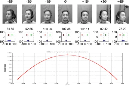
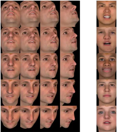
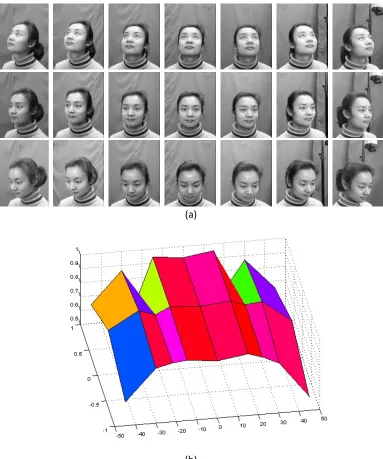
The Viola-Jones method is trained for locating faces of limited pose variation. As such, multiple passes over the image are required to find all faces, with each pass searching for a targeted range of pose. Empirical testing has shown that the default haarcascade_frontalface_alt2.xml classifier distributed with OpenCV [17] does a good job at detecting most faces over reasonable pose ranges. To demonstrate the effectiveness of the OpenCV implementation of face detection, the CAS-PEAL-R1 face database collected under the sponsor of the Chinese National Hi-Tech Program and ISVISION Tech. Co. Ltd. [18] was employed. This database contains multiple subjects photographed at three different levels of pitch and seven different yaw positions. An example subject from the CAS-PEAL-R1 face database is shown in Figure 2.1. (See Appendix I for a description of datasets used in this thesis.)

(16)

The Y-axis is pitch with a +1 meaning the subject was looking upward (approximately +30o pitch), a 0 meaning the subject was looking straight-ahead, and a -1 meaning the subject was looking downward (approximately -30o pitch). This classifier exhibited detection rates above 90% at near frontal yaw angles of all pitches, but performance degrades quickly with respect to pose. The two dips in performance at upward pitch and yaw of +/- 22o_{were due primarily to a limited number of samples at that particular pose}

position. Recent face detection methods incorporate pose and statistical models to improve the accuracy, efficiency, or robustness [19].

(a)

(b)

[image:16.612.115.498.219.678.2]

(17)

various yaw angle (X-axis) and pitch (Y-axis). The pitch on the Y-axis is defined as “1” looking up, ‘0’ looking straight, ‘-1’ looking down.

2.2

Facial

Feature

Point

Localization

After face detection, facial feature localization plays a prominent role in facial understanding. Facial feature detection algorithms include template matching methods [20], edge-based approaches, holistic methods [21], and shape models [22]. Shape models have the advantage that the shape of the face can be constrained to precisely locate key features of the face in the presence of occlusions. Statistical models capture shape variation, pose variation, and non-rigid deformations and envelope them via a linear model. Active Shape Models (ASMs), initially introduced by Cootes [23], have been enhanced by Bolin [24], and Milborrow [25]. Active Appearance models, initially introduced by [26] have been enhanced by Matthews [27], and are available as an open source software library (VOSM

http://www.visionopen.com/). Constrained Local Models (CLMs) [28] are similar to AAM models, but, they encode considerable pose and deformable face variations into a single model. Blanz [29] introduced the first 3D morphable models, and numerous 3D versions of each of the above shape models have since been proposed in the literature. Although the usage of 3D information often achieves slightly higher localization accuracy with only modest increase in compute power, 3D training data is still difficult to capture accurately for training and testing.

The ASM method localizes key facial landmarks, constraining each by plausible location learned from the training set. The AAM method furthers the ASM method by including location and appearance information while constraining each landmark, where the appearance information is defined by pixel intensity information defined by Delaunay triangulation between landmark points.

(18)

[image:18.612.104.520.72.288.2]

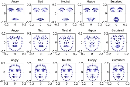
Fig. 2.2. Sample feature points produced by the ASM algorithm using Bolin [24] and Milborrow [25].

During training, the texture profile surrounding each feature point is learned from manually annotated ground truth subjects. The spatial relationship amongst feature locations is further used to develop a model which restricts the plausible region of each feature point. Figure 2.3 shows how the texture and statistical models are used by ASM during runtime. After face detection and eye localization, the eye centroid estimates along with the average face proportions are used to determine the approximate starting location for each feature point. The exact location of each feature point is determined by finding the point within the neighborhood search area that best matches the learned texture profile.

As shown in Figure 2.3, texture profiles are often defined as a 1D RGB gradient normal to the shape boundary. However, a second 1D gradient perpendicular to the first, and/or the surrounding neighborhood pixels of each feature point is also commonly used. The point with the smallest Mahalanobis distance with respect to the training data is selected as the search result, or feature point location. After all feature points are independently localized, the last step uses a holistic global shape model to constrain the overall shape. The global shape model transforms feature point locations to PCA space, where each dimension is constrained to be within +/- 3√λi, where λi is the eigenvalue that

corresponds to the ith_{eigenvector. The last three steps are repeated and generally converge after three to}

(19)

Fig. 2.3. Sample feature points produced by the ASM algorithm.

2.3

Facial

Pose

Estimation

Upon detection of the size and location of each face, there are many ways to perform facial pose estimation. A comprehensive survey of pose estimation techniques was documented by Muprhy-Chutorian [31]. This survey covered over 90 methods, loosely grouping them into eight categories: 1) Multiple face detectors, each tuned to a specific pose; 2) Direct comparison of filtered face to training exemplars; 3) Mapping of face features to pose classification or regression models; 4) ASM/AAM feature extraction to pose models; 5) Geometric models based upon eye/mouth/nose/etc landmarks; 6) Projection of facial features onto manifold surfaces; 7) Optical flow estimation from one video to the next; 8) Hybrid methods.

The pose estimation methods in this thesis rely heavily on dimensionality reduction. Performing dimensionality reduction on face pixels to estimate pose was demonstrated by [32-36]. Kanaujia [37] has shown that if we segment training samples by pose, and then utilize an intermediate step of first localizing facial features, we can build a family of principal components that enable a mixture of regression models.

Facial feature locations, such as corners of eyes, bottom of chin, etc., generally produce more accurate pose estimations than raw image pixels. ASMs were used for pose estimation in [38, 39] because they offer good feature localization and are robust over appearance variations and partial occlusions. Given accurate facial feature point locations, facial symmetry is very useful for pose estimation. For example, Figure 2.4 (left) shows the left eye length / right eye length, and Figure 2.4 (right) shows the left cheek area / right cheek area. Both are excellent predictors of yaw as they are generally invariant to pitch.

(20)

Fig. 2.4. (left) Using ASM eye points, calculate left eye length divided by right eye length for faces of various pose. (right) Using ASM points, calculate left cheek area divided by right cheek area for faces of various pose.

Recent pose detection approaches utilize 2D projection of 3D faces [40-42], 3D modeling of faces [43-45], and hybrid variations [46]. It remains a challenge to create techniques that are robust, accurate, and amenable to real time implementation. For example, most techniques fail in the presence of facial occlusions or harsh illumination, while others are computationally intensive.

2.4

Facial

Expression

Recognition

Facial expression recognition is the task of autonomously analyzing the human face to estimate a person’s emotional state, mood or other form of facial communication. The ability to automatically extract facial semantic information has widespread implications on a number of industries including security, entertainment, and human computer interfaces. State-of-the-art techniques have become adept at recognizing posed expressions in laboratory conditions and have migrated to recognizing spontaneous expressions in uncontrolled settings. These new techniques have the potential to improve the quality of life by offering easier and more efficient interfaces to machines as well as enabling new and exciting connections between humans.

(21)

survival necessity to the ability to fall in love and sustain relationships. Regardless of how they evolved, facial expressions have weaved their way into every corner of human to human communication.

In the late 1960’s, psychologist Paul Ekman, motivated by legendary professor Silvan Tomkins’s uncanny ability to read people’s faces, travelled the world and watched hundreds of thousands of facial film footage to understand human expressions. Ekman and his collaborator Wallace Friesen empirically proved all cultures exhibit the six universal expressions of fear, sadness, happiness, anger, disgust, and surprise. Ekman, Friesen, and their colleagues then created a taxonomy of facial expressions and documented forty-three facial movements constituting over ten thousand facial expressions. They discovered facial expressions consisted of both voluntary and involuntary muscle contractions, noted differences between genuine and posed expressions, and documented quick bursts of involuntary facial expressions called microexpressions. They further discovered that not only does mood or emotion involuntarily trigger facial muscle movements, but also performing an expression for extended periods evokes emotions related to that expression.

Computing power in the 1970’s and early 80’s was not powerful enough to tackle autonomous facial expression algorithms; but by the mid-1990’s computing advances enabled significant improvements in face detection and facial tracking, which reinvigorated interest in facial understanding research. Affective computing, or computing that deliberately senses and influences emotion, was brought to the forefront by Rosalind Picard’s book “Affective Computing” [4]. Gains in understanding facial expression and emotion have spawned a new era in human computer interfaces. Today, techniques are focusing on recognizing facial expression in unconstrained conditions that include variations of facial pose, facial occlusions, illumination, image fidelity, and background clutter.

2.4.1 Facial Expression Topology

Fig. 2.5. Minimal steps necessary for facial expression recognition.

The study of the six culture agnostic emotions, i.e. fear, sadness, happiness, anger, disgust, and surprise, has made great strides in recent years from constrained frontal posed faces to unconstrained faces in natural conditions [47-49]. Figure 2.5 shows the minimal steps necessary for a facial expression recognition system. Face detection, as described in Section 2.1, is often accomplished with the Viola-Jones [14] approach because of its low computational requirements and high detection rates. Following face detection, faces are normalized to a reference shape and size. Typically, the eye and mouth corners

Face Detection

Classification Engine Feature

Extraction Face

(22)

are localized, and an affine warp to canonical frontal face is defined. More complex methods utilize multiple canonical representations at various predefined pose representations [50].

Facial expression methods can be broadly categorized as geometric or appearance-based [51-53]. Geometric methods [54, 55] localize facial landmarks such as the outline of eyes, lips, nose, etc.. Appearance-based methods [56] work holistically with facial pixels enabling the capture of facial muscle subtleties such as nose wrinkles or dimple formation.

Geometric methods require computing size, shape, and location of key facial features such as the eyes, mouth, and eyebrows. Active Shape Model (ASM) or Active Appearance Model (AAM), as described in Section 2.2, are two of the most popular facial landmark localization methods [26]. Given enough training data and accurate facial landmark localization, shape models perform very well for expression classification [54, 55]. When the training set is not sufficiently rich, the trained ASM models may fail to capture the variance of individual expressions, which leads to reduced recognition performance. Furthermore, errors in point localization degrade expression classification accuracy further. Ptucha [57] demonstrated the effects of manually annotated vs. automatic ASM landmark placement on expression classification performance. Lucey [58] minimized this problem by applying neutral frame subtraction to the AAM points.

Appearance based methods often compute intermediate representations of images using features such as Gabor wavelets [59, 60] or Local Binary Patterns (LBP) [56, 61]. Gabor wavelets compute directional band pass filters based on the human visual system, but are slow and memory intensive. LBP capture various texture primitives and are quite tolerant to illumination changes. Shan [56] has shown that LBP slightly outperforms Gabor filters for expression recognition both in terms of speed and accuracy.

The classification engine for facial processing has been studied extensively [62]. With proper feature extraction, common methods such as k-Nearest Neighbor (k-NN), Support Vector Machines (SVMs), Logistic Regression, Adaboost, regression trees, and artificial neural networks yield acceptable results. Nonlinear methods or kernel-based methods generally offer small improvements. Sparse Representations (SRs) have proven to be effective at facial recognition, and recently have been adopted for facial expression classification [63].

(23)

motions and combinations of which enable final classification. Rather than attempt to interpret the facial emotion, FACS captures all the possible atomic facial signals that can then be used as features into a reasoning engine. For example, human subjects exhibiting AU six (contraction of orbicularis oculi and pars orbitalis, or the cheek raiser muscles) in combination with AU twelve (pulling up of the zygomatic major, or the corners of the lips) are generally experiencing happiness. Interestingly, Ekman discovered that if someone is asked to act as if they are happy, they perform only AU twelve. He found it almost impossible for subjects to exercise the orbicularis oculi and pars orbitalis properly on command. Equally intriguing, it was just as difficult for humans to stop those muscles from contracting when they were genuinely happy. Similar to FACS, the Moving Pictures Experts Group (MPEG) developed the Facial Animation Parameters (FAP) specification as part of the MPEG-4 international standard. FAPs are focused on animation of facial expression, but are strongly correlated with AUs used in FACS.

While it is not fully understood how the human brain determines the emotions of other faces, temporal evidence has been shown to significantly aid the true comprehension of the emotional state of faces [2, 64, 65]. Recent works have shown that temporal dynamics can improve AU detection considerably [66].

2.4.2 Facial Expression Classification

After face detection, ASM and AAM geometric methods automatically localize key facial features such as the eyes, mouth, and eyebrow boundaries. A generalized Procrustes analysis [67] on facial feature points compensates for translation, scaling (head size), and rotation (head roll), effectively transforming the set of facial points to a normalized canonical representation suitable for classification.

(24)

Fig. 2.6. Sample face exhibiting six pixel processing variants on top and block histograms on bottom. On the top, from left to right are luminance, edge magnitude, edge phase, LBP, Gabor, and LPQ.

Appearance based methods use eye and mouth corner points to define an affine warp transformation to a frontal canonical face representation. Edge gradients [68], Gabor wavelets [59, 60], Local Binary Patterns (LBP) [56, 61], and Local Phase Quantization (LPQ) [69] are common processing methods. Edge gradients typically use horizontal and vertical Sobel filters to extract edges of the face, resulting in the outline of eyes, nose, lips, etc. Gabor wavelets compute directional band pass filters inspired by properties of the human visual system. Typically, a multi-phase, multi-frequency bank of filters is used. Perhaps the most common configuration is eight equally spaced phases at five frequencies for a total of 40 Gabor representations. The Gabor representation in Figure 2.6 shows a mid-frequency filter at 45o_{. LBP captures various texture primitives and is quite tolerant to illumination changes. The}

LBP of a given pixel is obtained by comparing it with all pixels in a window centered at that pixel; if a window pixel is greater than the center pixel, it is encoded as a ‘1’. The concatenation of these binary comparisons forms a single binary number whose decimal equivalent is used as the LBP feature. LPQ has been shown to be quite tolerant to changes in image sharpness and illumination. LPQ computes the phases of low frequency coefficients whose histogram is used to derive the final feature representation. (Appendix II has a summary of pixel processing techniques used in this thesis.)

Another common feature used in appearance based facial expression models is block histograms. Block histograms divide the face into nr×nc (generally non-overlapping) regions, where nr and nc

represent the number of blocks down and across the face respectively. The histogram for each region is tabulated, and the histograms for all regions are concatenated to generate one large feature descriptor.

A facial region extraction and dimensionality reduction step may be added before feature extraction to make the model more general. The facial region extraction (see Section 6.2) allows the model to mask portions of the face. Processing individual facial regions is motivated by the need to

Luminance Magnitude Phase LBP Gabor LPQ

…

(25)

improve classification accuracy in the presence of occlusions and allows independent processing on each region of the face. When facial regions are used, block histograms are often unnecessary and each masked region is independently trained to obtain a localized model for every face region.

Regardless of whether geometric or appearance-based methods are considered, the features used in facial understanding often reside in representations of high dimensionality. These high dimensional feature spaces are inefficient and computationally intensive. Further, the artificially high dimensionality often masks the discriminative signal embedded in the data. As such, dimensionality reduction techniques are often utilized.

2.4.3 Dimensionality Reduction and Sparse Representations

Principal Component Analysis (PCA) and Linear Discriminant Analysis (LDA) are two effective techniques for obtaining a lower dimensional representation of the input data. PCA is used for unsupervised datasets and is optimal in the sense of reconstruction error. LDA is used for supervised datasets and is optimal in the sense of classification error. Both methods assume a linear mixture of Gaussian distributions. This may be limiting when modeling the behavior of complex imagery such as face representations.

Manifold learning techniques reduce the dimensionality of input data by identifying a non-linear lower dimensional space where the data resides [70, 71]. Popular methods include Isomap [72] and Locally Linear Embedding (LLE) [73]. In order to support the extension of the manifold model to new examples, linearized techniques such as Linear extension of Graph Embedding (LGE) [74], solve a linear approximation of the non-linear object. The dimensionality reduction offered by the LGE techniques generally affords greater dimensionality reduction than linear methods such as PCA or LDA.

The family of LGE techniques yields a multitude of dimensionality reduction techniques such as Locality Preserving Projections (LPP) [75] and Neighborhood Preserving Embedding (NPE) [76]. State-of-the-art techniques use a blend of supervised and non-supervised LGE techniques. The supervised techniques excel at class discrimination, and the non-supervised techniques more closely mimic the complex topology of spontaneous faces in uncontrolled conditions.

(26)

coefficient contamination issue without the need for neutral frame subtraction [79].

The communication between two humans often carries significant observable information that is best captured in a temporal fashion. Further, AU characterization in the FACS system assumes a neutral reference frame and includes levels of severity, making it ideally suited for temporal analysis. Both sparse and dense optical flow techniques across the human face can be incorporated into expression classifiers. Many of the same temporal techniques used for facial expression analysis pertain to gesture and action recognition. As such, the next section will cover temporal methods described in context of facial expression analysis, but all of which are suitable for gesture and activity analysis.

2.5

Temporal

Processing

The communication between humans naturally contains a temporal signature. For example, the rolling of the eyes, or raising of an eyebrow carries significant observable information that is best represented in a temporal fashion. Psychological studies have confirmed that temporal evidence is necessary towards the full comprehension of the emotional state of the face of interest [2, 64]. However, the usage of facial dynamics in the facial expression community is quite limited. As evidence of such, in the 2011 Facial Expression Recognition and Analysis Challenge (FERA2011), only four (out of fifteen) entrants utilized facial dynamics. Popular methods are extensions to static methods such as LBP-TOP [56] and LPQ-TOP [69].

The usage and interpretation of facial dynamics [64] by humans is an active area of research. Facial expressions typically contain an onset, apex, offset, and neutral stage. The timing and duration of each stage are critical to the interpretation of the observed behavior. These temporal dynamics have been used to discern between genuine and acted pain [80], telling the truth vs. lying [81], detection of depression [82], synthesizing facial expressions for avatars [83], and much more.

Facial dynamic methods include temporal tracking of geometric landmarks as well as tracking changes in facial appearance. Salient landmarks, such as corners of the eyes and mouth are generally well behaved and track well using optical flow techniques. Less well defined features, e.g. nose wrinkle, can be tracked with dense optical flow techniques such as Motion History Images (MHI) [84], Free Form Deformations (FFD) [85], or SIFT flow [86]. MHI was initially introduced for human movement recognition, and was later adopted for facial AU detection [66]. FFD was initially introduced for medical image registration and later adopted for facial AU detection [66]. SIFT flow was introduced for generic image registration [86], and adopted for face alignment [87].

Facial expressions or gestures can occur at any point in time and are variable in length. Thus, we

(27)

sequence, and l=1..m. Each of these temporal windows can be used as inputs to facial dynamic classifiers. Each temporal sliding window Wθl produces one of several estimates of facial expression per

video segment. These estimates are stored in a vector and converted into a single expression estimate via voting. Equation (2.1) combines static and temporal features into a single expression estimate:

Ψ · _∑ 2.1

Where Fs and Ft are the static and temporal vectors of predicted votes; hist() is a histogram operation; and

mode() computes the most frequently occurring prediction. Equation (2.1) weighs the votes of the static

model by the confidence values from the temporal model.

2.5.1 Facial Feature Point Tracking

When accurately placed, facial feature locations such as corners of eyebrows, outline of mouth, etc., can produce accurate expression estimations. Active Shape Models (ASMs) and Active Appearance Models (AAMs), initially introduced by [23] were used for expression estimation in [55, 88]. ASM is applied independently on each frame of the temporal window Wθl. For example, using the Bolin [24] ASM, we

get 82 facial feature points per frame. Each set of 82 points is transformed to a canonical face representation using a generalized Procrustes analysis [67]. With θ frames per Wθl, we get θ*82*2=θ*164

dimensions per each of the m samples.

Each sample is dimensionality reduced and classified using standard machine learning methods. The dimensionality reduction step not only reduces the upstream compute complexity, but also makes the sample data more discriminative, or more suitable for subsequent classification. The machine learning methods include techniques such as k-NN, regression trees, Support Vector Machines (SVM), neural nets,

etc. Alternatively, we can pass the average of the 82 points per Wθl into dimensionality reduction, or

convert these points to [Δx,Δy] or [magnitude,phase] motion vectors before dimensionality reduction.

2.5.2 Motion History Images

Motion History Images (MHI) were initially introduced for human movement recognition [84], and were later adopted for facial AU detection [66]. MHI compresses the motion over each sliding temporal

window Wθl into a single template. The methods described here are similar to [66], except the conversion

from MHI image to motion vectors is modified for improved facial expression performance. MHI initially evaluates the movement between all possible frames f and f+1 in Wθl, where f=1..θ-1. For each

(28)

, 1 | , , , , 1 |

0 2.2

where g(x,y,f) is a Gaussian filtered version of frame f and γ is a noise threshold. These difference frames are morphologically filtered with an opening operation to remove isolated noise. Each of the m sliding

windows produces a single frame called a MHIθl template:

1

1 max , 0 1 2.3

In this context, more recent movements are assigned higher weights. The MHIθl templates are

converted to motion vectors by replacing each pixel code value with a motion vector that points in the direction of the highest (most recent motion) code value within a 7x7 neighborhood. This neighborhood is constrained such that we may only point in the direction where pixels are monotonically increasing from the center outwards. Further, if there are several pixels of the same value, the average value is used.

ΔX, ΔY, magnitude, and phase-magnitude versions of this motion vector image are passed into dimensionality reduction.

Fig. 2.7. Sample anger (left) and joyful (right) temporal windows, θ=20. For each group: (upper left) movement of ASM facial feature points from first (red) to last (blue) frame; (lower left) corresponding MHI template; (right) final motion vectors from the MHI template.

2.5.3 Free Form Deformations

Free Form Deformations (FFD) are a dense optical flow technique initially introduced by [85] for medical image registration and later adopted for facial AU detection [66]. Given two images, FFD computes a rigid global motion and a non-rigid local motion model representing the movement of each pixel from one frame to the next. The global motion model iteratively solves for a 3x3 affine transformation matrix using convex optimization techniques across all pixels in both images. The local motion model solves for the displacement of a mesh of grid points. Given input pixel (x,y)t in frame t, we solve for the estimate of

(29)

(

x’

,

y’

)

t+1

= (

x,y

)

t

+

F

t

(

x

,

y

)

2.4

Ft(x,y) is solved for each pair of neighboring frames {f, f+1} in the temporal window Wθl, and

pass the set of all Ft(x,y) per Wθl as the input to dimensionality reduction. To solve for each Ft(x,y), FFD

solves a gradient descent optimization across a sparse mesh of control points, minimizing sum of square difference of pixels values. Given the deformed sparse mesh of control points, any interpolation method can solve for the dense motion Ft(x,y) at each input pixel location. FFD uses cubic B-splines as the

resulting fit is smooth and continuous across mesh vertices. To avoid local minima and make this process more computationally tractable, a hierarchical approach, solving from a low to high resolution mesh is utilized. Each mesh point position is initialized by the lower resolution mesh preceding it. Gaussian blurring with a σ twice the grid spacing at each level in the pyramid ensures robust behavior.

ASM

FFD

SIFT

flow

MHI

ASM

Classifier

FFD

Classifier

SIFT

flow

Classifier

(30)

Fig. 2.8. Sample temporal window Wθl , θ=4 frames, from an ‘angry’ video. From top to bottom we have input

60×51 cropped and affine warped faces, 82 point ASM motion vectors (black arrows have blue tail, red tip), grid of 28×24 dense FFD optical flow vectors, grid of 21x17 dense SIFT flow vectors, and MHI fields. For MHI three 60×51 difference frames form one 60×51 MHI template and one 30×26 dense MHI flow field.

2.5.4 SIFT Flow

SIFT flow [86] is an image alignment algorithm initially introduced to register two similar images and further adopted for facial registration by [86] [87]. Similar to FFD, SIFT flow produces a dense optical

flow field between all neighboring frames {f, f+1} in the temporal window Wθl. SIFT descriptors are

densely computed on every input pixel. The objective function of SIFT flow is similar to optical flow, but minimizes SIFT descriptors rather than RGB values:

(

)

∑

−

∑

−

∈ + + + + + = ε α α σ ) ,

( 1 1

2 2 2 1 ) , ) ( ) ( min( ) , ) ( ) ( min( ) ( ) ( 1 ) ( 2 ) ( 1 ) ( q p p p d q v p v d q u p u p v p u w p s p s w E

2.5

Where p represents all pixels in the image, s1 and s2 are the SIFT image for two neighboring frames, w is

the flow field in the u and v directions, ε is the local neighborhood of the pixel p with neighbor q. The first regularization term favors small displacements and the second discourages discontinuities in the local field. An iterative belief propagation algorithm is used to solve for w. Silimarly to FFD, a multi-grid

hierarchy is used both for speed and robust point matching. For the experiments in this thesis, σ=300,

α=0.5, and d=2.

2.6

Depth

Cameras

With the introduction of low cost depth cameras such as Microsoft Kinect [89], depth estimation has for the first time become an affordable option for digital interfaces. Depth information provides much more salient information than RGB or grayscale cameras for subject gesture recognition. The extraction of objects against backgrounds, and the tracking of objects have been simplified from a highly compute intensive and error prone task to one that is much more robust and works with much simpler methods [6]. To the average gamer, Kinect may be just another cool interfacing device, but for the computer vision world, Kinect has spurred a revolutionary leap in human-machine interaction.

(31)

Fig. 2.9. The Kinect sensor and standard drivers enable silhouette extraction of multiple users.

For example, Figure 2.9 shows three subjects interacting with a RGB camera on the left and depth camera on the right. Only moving objects are considered for extraction. The depth of the moving blobs against the static background is easy to extract using the depth channel and conventional computer vision algorithms such as temporal thresholding. At this point, any moving object is a candidate for extraction- a cat, dog, moving car, etc., would all be extracted as a contiguous object. Further, humans carrying tools or other objects, or wearing loose clothing or objects such as backpacks would expand the range of the deformable object. For the system to work properly in this thesis, the only moving objects should be humans, and all humans should avoid wearing loose clothing or holding anything that could easily trick the silhouette extraction software.

Given the silhouette of a human, each section of the silhouette blob needs to be assigned to a body part, where kinematic and temporal constraints ensure plausible limb identification. A skeletal model is then fit to localize the ankles, knees, hips, shoulders, elbows, wrist, head and torso. The model employed by Kinect is documented in [6].

The first step is to assign each pixel in the silhouette map to one of thirty-one predefined body parts. To increase saliency, the silhouette map is converted to a depth delta map, where the difference in depth between each pixel and its neighbors is used as a classification feature. The classification engine is a training forest of decision trees, each trained with over one-million manually labeled ground truth samples. Each decision tree is pruned to a depth of twenty. After each pixel in the silhouette is classified independently by the decision forest, neighborhood filtering classifies each pixel as belonging to one of the thirty-one body parts. The joint position can’t be determined by 3D centers of probability mass because of sensor noise and shadowing caused by triangulation of the IR emitter and detector used in the depth camera. Instead, a local mode-finding approach based on mean shift with a weighted Gaussian kernel is used.

(32)

Shotton claimed that even if all joints were tracked with 99% accuracy, after one minute the skeleton would be grossly misrepresented 50% of the time. As such, an independent joint assignment is made on each video frame, and then kinetic and temporal smoothing constraints are imposed.

2.7

Gesture

Recognition

Nonverbal gestures can be used in place of voice commands both because of the natural tendencies of humans, as well as unpredictable sound in crowded or busy environments. Gestures include movement of the arms, hands, and face. Although many gestures are culture agnostic, researchers will no doubt develop new variants of gestures which users find natural and intuitive to perform. These gestures are likely to change by application, environment, and culture. For example, gestures in games may include simulation of shifting a car and turning a steering wheel, while gestures in an airport may only include simple point and select of airline departure times.

By extracting head pose, calculating depth, then using Euler angle geometry [90], we can project a human’s visual focus of attention onto the screen. Similarly, by using joint locations and projecting a line fit through the shoulder and arm joints onto the screen, we can estimate where the human is pointing. Empirical studies have shown that head pose is more appropriate for displays of close proximity, while pointing is more intuitive than using the head pose for larger displays, or displays that are further away. Because no two humans are the same size/shape, and because systems are subject to calibration/perspective errors, a fiducial should be placed on the screen, indicating where the actor is looking/pointing.

Fig. 2.10. Skeleton overlay on top of RGB image.

(33)

The most intuitive gestures mimic familiar physical interactions, which makes high accuracy and low latency paramount to meeting user’s expectations for usability and feedback [95]. Using only tightly constrained body gestures has been shown to reduce the usability of highly interactive applications with many degrees of freedom [96], such as video games. Heydekorn et al. [97] have shown that more constrained application specific gestures are less intuitive than loosely constrained gestures for users. To accomplish these goals, new methods that are capable of both accurate classification and real time implementation are necessary.

Action classification requires descriptors that are both discriminative and computationally efficient. Spatial action representations, such as body models [98], body pose estimations [99], kinematic joint models [100], and stick figures [101] offer intuitive representations, but may not adequately capture the human body’s high degree of variability. Spatial parametric image features such as contour/silhouette representations [102] and optical flow [103] don’t require body part labeling or tracking, but are more computationally intensive.

Temporal modeling methods for gesture control include temporal tracking of skeletal joints as well as dense tracking of RGB or depth pixels. Dense optical flow techniques include Motion History Images (MHI) [84], Free Form Deformations (FFD) [85], and SIFT flow [86] as reviewed in Section 2.5.

This thesis introduces active difference signatures to select active temporal regions of interest based on both the depth map from a 3D camera along with estimated kinematic joint positions [6]. The skeletal joints are normalized using a reference representation of both the depth image and the joint locations. The difference between the normalized joints and a canonical representation of skeletal joints forms an active difference signature, a salient feature descriptor across the video sequence. This descriptor is dynamically time warped to a fixed temporal duration in preparation for classification.

2.8

Notation

Variables, vectors, and matrices are denoted with italics. Matrices are bold uppercase, and vectors are bold lowercase. Components of vectors are denoted with subscripts such as xn, for the nth offset of vector

x. Matrices are denoted with subscripts such as Wij, to represent the ith row and jth column entry of matrix W. Images are treated identically as matrices. Matrices and images are stored in lexicographic form before being input into classifiers. The dimensionality of a vector is denoted as x∈RD_{, meaning that}

vector x has D dimensions or D entries. The dimensionality of a matrix or image area is denoted as

X∈RD×n_{, meaning that matrix}_X_has_n_{entries, each of}_D_{dimensions. The}_ℓ0_{norm of a vector}_x_∈_RD_{is a}

sparsity measure which counts the number of non-zero vector elements as ∑ | | . The ℓp

(34)

matrix X∈RD×n_{is defined as} _∑ _∑ _, _{. Common variables used throughout this}

thesis include:

n: The number of (training or testing) samples.

k: The number of discrete classes for a dataset.

D: The (high) dimensional of a feature before dimensionality reduction.

d: The (low) dimension of a feature after dimensionality reduction.

U: A D×d dimensionality reduction matrix.

W: A n×n adjacency matrix that represents neighbor to neighbor connections from each of the n

input samples to all other n-1 samples in a dataset.

Φ: A sparse representation dictionary.

a: The sparse coefficients, or linear amounts used from each element in the dictionary

m: The number of entries in a sparse representation dictionary Φ.

λ: The regularization parameter used in sparse representation, 0 ≤ λ ≤ 1. Higher values of λ

induce more sparsity.

α: The semi-supervised parameter used in dimensionality reduction, 0 ≤α ≤ 1. Lower values of

α use more unsupervised dimensionality reduction. Higher values of α use more supervised dimensionality reduction.

(35)

3

Dimensionality

Reduction

Dimensionality reduction maps data of high dimension to a lower dimension, and often discards uninformative variance. This process makes the data more compute friendly, removes noise, emphasizes discriminative properties, and enables improved inference for later regression or classification models. Complex objects such as facial images often necessitate representations of high dimensionality. For example, Lucey [58] represents faces using 68 landmark points and 87×93 pixels. As a result, each face resides in RD_{where D=(68}_×₂₊₈₇_×_{93)=8,227. This high dimensional feature space is not only inefficient}

and computationally intensive, but the sheer number of dimensions often masks the discriminative signal embedded in the data.

Formally, the input feature space contains n samples, x1, x2, …xn, each sample of dimension D, xi ∈RD_{. These}_n_{samples are projected onto a lower dimensional representation, yielding}_y

1, y2, …yn, each

output sample of dimension d, yi∈Rd. As d is always ≤D, we are interested in the case where d << D.

In matrix notation, the input feature space is described by n×D matrix X, where the ith_{row of}_X

corresponds to xi. In the linear projection from D to d dimensions, we have YT=XTU, X∈RD×n, Y∈Rd×n,

and U is the D×d projection matrix.

3.1

PCA

Principal Component Analysis (PCA) is the most often used dimensionality reduction method and often serves as a starting point for many dimensionality reduction methods. PCA is an unsupervised linear dimensionality reduction method that projects data along orthogonal directions of maximum variance. PCA is optimal in the sense of reconstruction error, but PCA basis functions are not usually optimal for feature extraction or discriminative classification.

PCA solves for one dimension at a time according to yi = UiTxi, where each Ui maximizes:

max 3.1

and

1

3.2

(36)

, ∑

1 3.3

As such, cov(a,a) = var(a), and cov(a,b) = cov(b,a). When cov(a,b) > 0, it indicates that as a

increases, so does b. For D-dimensional data, we need to calculate D!/(2(D-2)! covariance values and D

variance values. A good way to store these values is in a D×D matrix. For example, for 3-dimensional data, we have:

, , ,

, , , 3.4

The diagonals are all the variances. Since cov(a,b) = cov(b,a), the matrix is symmetric. The eigenvectors of the covariance matrix C form the basis functions that convert to the alternate space (which in this case maximizes variance). The eigenvector defines the projection vector and the corresponding eigenvalue defines the variance of the data after it is projected onto the eigenvector. D dimensional data yields a D×D covariance matrix and D eigenvector/eigenvalue pairs. The eigenvector with the largest eigenvalue is called the principal component. Eigenvectors are generally sorted from most to least significant, according to the eigenvalues. As such, the eigenvector matrix is D×D, consisting of D

column eigenvectors, where each eigenvector is a D×1 projection vector. As such, U consists of D

eigenvectors, each eigenvector being D×1.

If we format the n input samples, x, into n column-wise samples, each sample of dimension D, we obtain a D×n input matrix X. Then YT₌_XT_U_{, where}_Y_{is the PCA transformed space,}_U_{is the matrix of}

eigenvectors, and X is the input data. Each output sample (row of) Y is a linear combination of the D dimensions of each input sample (columns of X), and so PCA is a linear transform. Given Y, we can transform back to X using XT₌_YT_U-1_{. Since the inverse of an orthogonal matrix is its transpose, we have} XT=YTUT, another useful property of PCA.

The eigenvectors of PCA are alternate basis functions that can be used to represent the input data. Often we only need to use d eigenvectors, and the remaining (D-d) eigenvectors and corresponding eigenvalues are 0. In such cases, we reduce the basis or dimensionality of the data from D to d without information loss.

For usage in computer vision classification, verification, or recognition, it will be shown that an object can be reconstructed from a training dictionary of similar objects:

(37)

where μ is the mean object from the training dictionary, φ is the number of training samples in the dictionary, a is the coefficient weight, and Φ is the training sample dictionary. This is analogous to the PCA transformation where we construct a linear transformation of D eigenvectors. The key difference is

how we weight each eigenvector Φι by ai. The vector of coefficients a, are a unique signature of x and

can be used to identify an object. Solving for a is best done via an example.

Assume n=100 samples and each sample consists of 50x50 pixels. We can represent each sample as a one dimensional vector of D=2500 dimensions giving an D×n feature matrix A. Computing the covariance of A results in a 2500×2500 covariance matrix C=AT_A_{which may cause the computer to run}

out of memory. Alternatively, we can compute matrix L=AAT_{, which is only 100}_×_{100. We can work}

with L instead of C because the eigenvectors of L are linear combinations of the eigenvectors of C. An alternate representation of the eigenvectors of C is Uc=Aeig(L). In this fashion Uc is a 2500×100