This is a repository copy of
Improved model identification for nonlinear systems using a
random subsampling and multifold modelling (RSMM) approach
.
White Rose Research Online URL for this paper:
http://eprints.whiterose.ac.uk/74619/
Monograph:
Wei, H.L. and Billings, S.A. (2007) Improved model identification for nonlinear systems
using a random subsampling and multifold modelling (RSMM) approach. Research Report.
ACSE Research Report no. 962 . Automatic Control and Systems Engineering, University
of Sheffield
[email protected] https://eprints.whiterose.ac.uk/ Reuse
Unless indicated otherwise, fulltext items are protected by copyright with all rights reserved. The copyright exception in section 29 of the Copyright, Designs and Patents Act 1988 allows the making of a single copy solely for the purpose of non-commercial research or private study within the limits of fair dealing. The publisher or other rights-holder may allow further reproduction and re-use of this version - refer to the White Rose Research Online record for this item. Where records identify the publisher as the copyright holder, users can verify any specific terms of use on the publisher’s website.
Takedown
If you consider content in White Rose Research Online to be in breach of UK law, please notify us by
Research Report No. 962
Department of Automatic Control and Systems Engineering The University of Sheffield
Mappin Street, Sheffield, S1 3JD, UK
September 2007
Improved Model Identification for Nonlinear Systems
Using A Random Subsampling and Multifold
Modelling (RSMM) Approach
H. L. Wei and S. A. Billings
The University of Sheffield
Mappin Street, Sheffield
S1 3JD, UK
[email protected], [email protected]
Abstract: In nonlinear system identification, the available observed data are conventionally
partitioned into two parts: the training data that are used for model identification and the test data that
are used for model performance testing. This sort of ‘hold-out’ or ‘split-sample’ data partitioning
method is convenient and the associated model identification procedure is in general easy to
implement. The resultant model obtained from such a once-partitioned single training dataset, however,
may occasionally lack robustness and generalisation to represent future unseen data, because the
performance of the identified model may be highly dependent on how the data partition is made. To
overcome the drawback of the hold-out data partitioning method, this study presents a new random
subsampling and multifold modelling (RSMM) approach to produce less biased or preferably unbiased
models. The basic idea and the associated procedure are as follows. Firstly, generate K training datasets (and also K validation datasets), using a K-fold random subsampling method. Secondly, detect significant model terms and identify a common model structure that fits all the K datasets using a new proposed common model selection approach, called the multiple orthogonal search algorithm. Finally,
estimate and refine the model parameters for the identified common-structured model using a
multifold parameter estimation method. The proposed method can produce robust models with better
generalisation performance.
Keywords: Cross-validation, model structure/subset selection, nonlinear system identification,
parameter estimation, random resampling, split-sample.
1. Introduction
A mathematical model of a nonlinear dynamical system is usually defined by two properties: the
model structure and the associated model parameters. The central task in any nonlinear system
identification task is to construct, based on available observations, a suitable model structure using
some specified elementary building blocks, and then to calculate the associated model parameters
using some linear or nonlinear parameter estimation algorithm. Take the commonly used
to describe the underlying system, and where candidate model terms or regressors are formed by some
linear or nonlinear combinations of lagged input and output variables. The initial full regression model
may be very complex and will typically include a great number of candidate model terms and some
efficient model structure selection procedures, using either the best subset or stepwise search methods,
will need to be performed to determine which model terms are important and should be included in the
model. The forward stepwise regression method, especially the well known orthogonal forward
regression (OFR) type methods (Billings et al. 1989b, Chen et al. 1989), have been widely employed
in recent years for model structure identification of nonlinear dynamical systems (Leontaritis and
Billings 1987, Billings et al. 1989a, Billings and Chen 1989, Chen et al. 1992, Zhu and Billings 1993,
1996, Billings and Zhu 1994, Aguirre and Billings 1994, 1995a, b, Chen et al. 1996, Billings and Chen
1998, Correa et al. 2000, Harris et al. 2002, Hong et al. 2003a,b,c, Wei et al. 2004, Tsang and Chan
2006, Truong et al. 2007).
Conventionally, the available observational dataset is often partitioned into two parts: the training
data that are used for model identification including parameter estimation, and the test data that are
used for model performance testing. The main advantage of this sort of ‘hold-out’ or ‘split-sample’
data partitioning method is that it is convenient and the associated model identification procedure is in
general easy to implement. Notice, however, that the division of the training and test data using the
‘hold-out’ method, for model identification, may sometimes be subjective and models produced by the
once-partitioned single training dataset may occasionally be biased, because the identified model
structure and the estimated model parameters can be highly dependent on how the given dataset was
partitioned. The most useful approach, to overcome the drawbacks of the hold-out method for
nonlinear dynamical modelling, is to introduce cross-validation, which has been extensively applied in
conventional linear regression and related models (Allen 1974, Stone 1974, Golub et al. 1979, Shao
1993), into the model identification procedures (Stoica et al. 1986, Ljung 1987). In fact, leave-one-out
(LOO) cross-validation has been introduced for model parameter estimation of nonlinear regression
models (Hansen and Larsen 1996, Myles et al. 1997, Monari and Dreyfus 2002) and for model
construction of linear-in-the-parameters regression models for nonlinear dynamical systems (Hong et
al. 2003a,b,c, Chen et al. 2004). It has been shown that by incorporating the LOO cross-validation in
the OFR procedure, the resultant algorithms can often produce efficient sparse models for nonlinear
identification problems using the linear-in-the-parameters regression form of models (Chen et al.
2004). Recent applications of the forward or backward orthogonal selection algorithms, assisted by the
LOO criterion, can be found in Truong et al. (2007) and Hong and Mitchell (2007). A variation of the
conventional LOO criterion for model subset selection of nonlinear systems can be found in Billings
and Wei (2007). An attractive advantage of LOO for dealing with linear least squares problems is that,
a closed form solution is available to calculate the associated LOO criterion from the results of a
single least-squares fit to all training samples.
expected generalisation error (Stone 1974, Efron and Tibshirani 1993), the associated variance may be
very large (Efron 1983, Breiman 1996). Another drawback of the LOO cross-validation is that it is
unstable with respect to small perturbations in the data, that is, a slight data perturbation may lead to a
drastic change in the resultant regression models (Breiman 1996). Furthermore, LOO cross-validation
also has some more subtle deficiencies in model subset selection. For example, it has been shown
(Shao 1997) that for linear regression models, LOO is asymptotically equivalent to the AIC and
Mallow’s Cp criteria; however, leave-v-out cross-validation, is asymptotically equivalent to Schwarz’s Bayesian information criterion (BIC), for some specifically chosen v. It is known that, with the same subset selection procedure, the number of model regressors chosen by using the AIC criterion is
always greater than that chosen by using the BIC criterion. Results from numerous simulations have
shown that while AIC tends to produce badly overfitted models with a small number of training
samples, BIC can still work well (Hurvich and Tsai 1989, Shao and Tu 1995). This suggests that
leave-v-out cross-validation, with some appropriately chosen values for v, should provide better results, for linear regression models.
Leave-one-out cross-validation can be viewed as the extreme case of K-fold cross-validation where
K is is equal to the number of involved observations. The aforementioned discussions suggest that K -fold cross-validation should be superior to LOO cross-validation, in the sense that K-fold cross-validation could produce robust regression models with better generalisation properties. In fact,
Breiman and Spector (1992) found that, for subset selection and evaluation in linear regression
modelling, five- or ten-fold cross-validation (leave out 20% or 10% of the data) gave better results
than LOO.
With the aforementioned observations and keeping in mind that prediction accuracy is often the
‘gold standard’ for model identification, this study aims to present a new random subsampling and
multifold modelling (RSMM) approach to produce robust models with better generalisation properties.
The implementation of the RSMM method consists of three stages. The first stage involves data
resampling, which is quite similar to K-fold random cross-validation. At this stage, K training datasets are independently generated; each dataset contains a certain number of data points that are randomly
selected from a specified dataset. Corresponding to each training dataset, a validation dataset can be
obtained by removing the training data points from the specified dataset. The second stage involves
the detection of common significant model terms and the identification of a common model structure
that fits all the K datasets. A new common model selection approach, called multiple orthogonal search (MOS) algorithm, is proposed to achieve the target of this stage. The objective of the third
stage is to refine the associated model, by applying a multifold parameter estimation approach to the
identified common-structured model, to produce some improved estimates of the model parameters.
The paper is organised as follows: In section 2, the linear-in-the-parameters regression model is
briefly presented. In section 3, the three stages are presented in detail. Some examples are provided in
of nonlinear systems. The paper ends with summary in section 5, where some comments are given.
2. The Linear-In-The-Parameters Model
Consider the identification problem for nonlinear systems given N0 pairs of input-output
observations,{(u(t),y(t)):t=1,2,L ,N0}, where u(t) and y(t) are the observations of the system input
and output, respectively. The relationship between the input and the output of a wide class of nonlinear
systems can formally be described using the NARX (Nonlinear AutoRegressive with eXogenous
inputs) model below (Leontaritis and Billings 1985, Pearson 1995, 1999, Ljung 2001)
) ( )) ( , ), ( ), ( , ), 1 ( ( )
(t f yt y t n u t ut n et
y = − L − y L − u + (1)
where f is some nonlinear function, nuand ny are the maximum lags in the input and output, respectively, and e(t) is an independent identical distributed noise sequence.
The function f is in general unknown and needs to be identified from given observations of the system. The task of system identification is thus to find, from the given data, a nonlinear approximator
fˆ that can represent the true (but unknown) function f. Generally, the identified model should not
only fit the observed data accurately, but also possess good generalization properties, meaning that the
model is capable of capturing the underlying system dynamics, so that the model can be used for
simulation, prediction, and control. One commonly used approach, for effectively reconstructing the
nonlinear function f, is to construct a nonlinear approximator fˆ using some specific types of basis
functions including polynomials, radial basis functions, kernel functions, splines and wavelets
(Leontaritis and Billings 1987, Chen and Billings 1992, Brown and Harris 1994, Murray-Smith and
Johansen 1997, Cherkassky and Mulier 1998, Liu 2001, Harris et al. 2002, Wei and Billings 2004,
Billings and Wei 2005). More often, models constructed using these methods can easily be converted
into a linear-in-the-parameters form, which is an important class of representations for nonlinear
system identification, because compared to nonparameters models,
linear-in-the-parameters models are simpler to analyze mathematically and quicker to compute numerically.
Let d=ny+nu and
T d t x t x t x
t) [ (), ( ), , ()]
( = 1 2 L
x with
≤ ≤ + −
−
≤ ≤ −
=
d k n n
k t u
n k k
t y t x
y y
y k
1 )) ( (
1 ) ( )
( (2)
) ( ) ( ))
( ( ˆ ) (
1
t e t t
f t y
M
m m
m +
=
=
∑
= φ θ
x =φT(t)θ+e(t) (3)
where M is the total number of candidate regressors, φm(t)=φm(x(t))(m=1,2, …, M) are the model
terms generated, in some specified way, by the elements of the ‘input’ (predictor) vector x(t),θmare
model parameters, and φ(t)=[φ1(x(t)),L ,φM(x(t))]T and θ are the associated regressor and
parameter vectors, respectively. Notice that in most cases the initial full regression equation (3) might
be highly redundant, some of the regressors or model terms can thus be removed from the initial
regression equation without any effect on the predictive capability of the model, and this elimination
of the redundant regressors usually improves the model performance. Generally, only a relative small
number of model terms need to be included in the regression model for most nonlinear dynamical
system identification problems. An efficient model term selection algorithm is thus highly desirable to
detect and select the most significant regressors.
3. The Random Subsampling and Multifold Modelling Approach
The random subsampling and multifold modelling (RSMM) approach consists of three steps:
random subsampling, common model structure identification and model parameter estimation.
3.1 Random subsampling
Random resampling methods, including cross-validation, bootstrapping and jackkniffing (Devijver
and Kittler 1982, Efron and Gong 1983, Efron and Tibshirani 1993), have been widely applied for data
analysis and nonparametric modelling tasks. This study, however, employs a K-fold random subsampling method to generate, from a set of chronologically recorded observations, a number of
training and validation datasets, which are to be used for model identification including parameter
estimation of nonlinear systems.
Consider the model identification problem for a nonlinear dynamical system, whereN0pairs of
observations,{(x(t),y(t)):t=1,2,L ,N0}, are available. Following the conventional routine of the
‘hold-out’ method, theN0data pairs are first split into two parts: the training dataset consisting of the
first N data pairs, and the test dataset consisting of the remaining N0−N data pairs.
Let B= ξ{ t:t=1,2,L ,N} and T= ξ{ t:t=N+1,L ,N0}, where ξt =(x(t),y(t)) is the t-th sample
(observation pair). Following the idea of conventional cross-validation, samples in the dataset B can be resampled as follows:
• K-fold cross-validation. The dataset B is split, along the coordination of the sampling index t, into
K subsets, with roughly equal data length (number of samples). The hold-out method is then repeated K times, and at each time, one of the K subsets is used as a validation set and the other
• K-fold random subsampling. The dataset B is randomly partitioned into K different subsets; each subset contains a certain number of samples that are randomly selected (without replacement) from
B. Each of the K subsets is successively used as a validation set.
This study considers the K-fold random subsampling method, which is implemented as below.
• Step 1. Let Γ0={1,2,L ,N}and Γ={i:i∈Γ0} be a random permutation of Γ0. Divide the index set
Γ into K different parts, Γ1,Γ2,L ,ΓK, where each part is roughly with the same size.
• Step 2. LetVk ={ξt:ξt∈B,t∈Γk} andBk =B\Vk ={ξt:ξt∈B,t∈Γ\Γk}, with k=1,2, …,K. Each
k
B is used as a training set and each Vk is used as a validation set.
For the givenN0pairs of samples{ξt=(x(t),y(t)):t=1,2,L ,N0}, both the associated training dataset
} , , 2 , 1 :
{ t N
B= ξt = L and the K training sets B1,B2,L ,BK , along with the K validation sets
K
V V
V1, 2,L , , will be used to identify an appropriate regression model of the form (3) for the relevant
dynamical system. This will be achieved with a new multiple orthogonal search algorithm (MOS)
below.
3.2 The multiple orthogonal search algorithm for model selection
From the above discussion, it is known that all the datasets B1,B2,L ,BKand V1,V2,L ,VKcome
from the same dynamical system. These datasets should thus share, in theory, the same model
structure, as well as the same model parameters. At the moment, however, the common model
structure is not yet known and needs to be identified from these given datasets.
Let the number of samples in the training dataset Bk be Nk, and denote these Nksamples by
: )) ( ), ( (
{ξk,t= xk t yk t ξk,t∈Bk, t=1,2,L ,Nk}. The objective is to identify a common-structured
sparse model, for the given system, from the following multiple regressions
) ( )) ( ( )
(
1
, t e t
t
y k
M
m
k m m k
k =
∑
+=
x
φ
θ ( ) ( )
1 ,
, t ek t
M
m
m k m
k +
=
∑
=
φ
θ (4)
whereφk,m(t)=φm(xk(t)), with k=1,2, …, K, m=1,2, …, M, and t=1,2, …, Nk. These equations can be
expressed using a compact matrix form below
k k k
k θ e
y =Φ + (5)
whereyk =[yk(1),L ,yk(Nk)]T,θk =[θk,1,L ,θk,M]T,ek =[ek(1),L ,ek(Nk)]T, and Φk =[φk,1,L ,φk,M]
with T
k m k m
k m
k, =[φ , (1),L ,φ , (N )]
φ for k=1,2, …, K and m=1,2,…, M.
3.2.1 Multiple orthogonal search (MOS) for model term selection
The multiple orthogonal search (MOS) method, which can be considered as an extension of the
1989), is developed to select a common-structured sparse model from the multiple regressions given
by (4) and (5). LetI={1,2,L ,M}, and denote by D= φ{ m:m∈I} the dictionary of candidate model
terms. For the kth training dataset Bk , the dictionary D can be used to form a dual
dictionaryDk ={φk,m:m∈I}, where the mth candidate basis vector φk,m is formed by the mth
candidate model termφm∈D, in the sense that φk,m=[φm(xk(1)),L ,φm(xk(Nk))]T (k=1,2, …,K). The
common model term selection problem is equivalent to finding, from the dictionaryD= φ{ m:m∈I}, a
subset D
n
s s
s , , , }⊂
{
2
1 φ φ
φ L (generallym<<M ), so that yk (k=1,2, …, K) can be satisfactorily
approximated using a linear combination of {φk,s1,φk,s2,L ,φk,sn}⊂Dk as
k s k n k s k k
k φ φ n e
y =θ ,1 ,1+L +θ , , + (6)
The MOS algorithm selects significant model terms in a forward stepwise way, one model term at
each search step. Initially, letrk,0=yk(k=1,2, …, K). For k=1,2, …, K and j=1,2, …, M, calculate
) )( ( ) ( ) , ( err , , 2 , ) 1 ( j k T j k k T k j k T k j k φ φ y y φ y
= (7)
and define =
∑
= ≤ ≤ K k Mj K k j
s 1 ) 1 ( 1
1 err ( , )
1 max
arg (8)
The first significant common model term can then be selected as the s1th element,
1
s
φ , in the
dictionary D. Accordingly, the first significant basis vector for the kth regression model is thus
1
, 1 , ks
k φ
α = , and the associated orthogonal basis vector can be chosen as
1
, 1 , ks
k φ
q = .The model
residual for the kth regression model, related to the first step search, is given as
1 , 1 , 1 , 1 , 0 , 1 , k k T k k T k k k q q q q y r
r = − (9)
In general, the mth significant model term m
s
φ can be chosen as follows. Assume that at the (m-1)th
step, (m-1) significant model terms, φ1,φ2L ,φm−1, have been selected. Letαk,1,αk,2,L ,αk,m−1be the
associated basis vectors for the kth regression model, and assume that the (m-1) selected bases have been transformed into a new group of orthogonal bases qk,1,qk,2,L,qk,m−1via some orthogonal
∑
− = − = 1 1 , , , , , , ) ( , m s s k s k T s k s k T j k j k m j k q q q q φ φp , j∈Jm (10)
whereJm={j:1≤ j≤M,j≠st,1≤t≤m−1}. For k=1,2,…,K and j∈Jm, calculate
] ) )[( ( ) ( ) , (
err ( )
, ) ( , 2 ) ( , ) ( m j k T m j k k T k m j k T k
m k j
p p y y p y
= (11)
and define =
∑
= ≤ ≤ K k m M jm k j
K s
1 ) ( 1 err ( , )
1 max
arg (12)
The mth significant common model term can then be selected as the smth element, m
s
φ , in the
dictionary D. Accordingly, the mth significant basis vector for the kth regression model is thus
m s k m k, φ ,
α = , and the associated orthogonal basis vector can be chosen as , (,) m
s k m
k p m
q = .The model
residual for the kth regression model, related to the mth step search, is given as
m k m k T m k m k T k m k m k , , , , 1 , , q q q q y r
r = − − (13)
Notice that err(m)(k,sm) can be explained as the error reduction ratio (ERR) that is introduced by
including the mth basis vector
m
s k m
k, φ ,
α = into the kth regression model. The criterion (12), by
maximizing the sum of the ERR values, relative to all the K data sets, guarantees that the variation of the outputs in all the K data sets can be explained by including the model term
m
s
φ , with the highest
percentage, compared with selecting any other candidate model term φ∈D={φm:m∈I}. The
quantity
∑
= = K k m m s k Km) (1/ ) 1err( )( , )
AERR( (14)
is referred to as the mth average (or overall) error reduction ratio (AERR).
Subsequent significant bases can be selected in the same way step by step. Once the first (m-1) basis vectors αk,1,αk,2,L ,αk,m−1 (respectively the associated orthogonalized bases qk,1,qk,2,L ,qk,m−1)
have been determined, then these (m-1) bases together with the mth basis
m
s k m
k, φ ,
α = (respectively
the orthogonalized basis , (,) m
s k m
k p m
q = ) , can explain the variation in the outputs of the K data sets with
a higher percentage than by including any other candidate bases. This step-by-step forward selection
algorithm is a non-exhaustive search method, and may not always produce the global optimal solution.
From the above orthogonal procedure, it is known that the vectors rk,mand qk,m are orthogonal, thus m k T m k m k T k m k m k , , 2 , 2 1 , 2 , ) ( || || || || q q q y r
r = − − (15)
By respectively summing (13) and (15) for m from 1 to n, yields
n k n m m k m k T m k m k T k k , 1 , , , , r q q q q y y
∑
= += (16)
n k T n k n k T k n k n k , , 2 , 2 1 , 2 , ) ( || || || || q q q y r
r = − −
∑
=
−
= n
m km
T m k m k T k k
1 , ,
2 ,
2 ( )
|| || q q q y
y (17)
Equation (16) shows that yk can be approximated using a set of orthogonal vectors {qk,1,qk,2,L ,qk,n},
which are transformed from the original vectors ks ks ks k n}⊂D ,
, ,
{ , , ,
2
1 φ φ
φ L . The norm ||rk,n||2, or
some associated variations, is often used to form a criterion to determine the model complexity (model
size) in some conventional identification procedure, where observed data are partitioned using the
‘hold-out’ method. In this study, however, a K-fold random subsampling method is used to determine the model complexity.
3.2.2 Parameter estimation of individual models
It is easy to verify that the relationship between the selected bases ks ks ks k n}⊂D ,
, ,
{φ ,1 φ ,2 L φ , and
the associated orthogonal basesqk,1,qk,2,L ,qk,n, for the kth data set, is given by
n k n k n
k, Q , R ,
A = (18)
where Ak =[φk,s1,φk,s2,L ,φk,sn] , Qk,n is an Nk×n matrix with orthogonal columns
n k k
k,1,q ,2, ,q ,
q L , and Rk,n is an n×nunit upper triangular matrix whose entries are calculated during
the orthogonalization procedure. The unknown parameter vector, denoted by θk,n=[θk,1,L ,θk,n]T, for
the regression with respect to the original bases, can be calculated from the triangular equation
n k n k n k, θ, g ,
R = where gk,n=[gk,1,L ,gk,n]T and ( , )/( , k,m) T m k m k T k m
g = y q q q for m=1,2, …, n.
3.2.3 Model size determination
Model selection criteria are often established on the basis of estimates of prediction errors, by
inspecting how the identified model performs on future (never used) data sets. Several criteria, for
example, the Akaike information criterion (AIC) (Akaike 1974), the Bayesian information criterion
(BIC) (Schwarz 1978), the minimum description length (MDL) (Rissanen 1978), the generalised
Stoica and Selen 2004), are available to determine the model complexity or model size (number of
regressors). In this study, however, one variation of the conventional BIC (Efron and Tibshirani 1993)
is considered, and this given as below
) MSE( ) ln( 1 ) BIC( p p N N p p − + = N p N N
pln( ) RSS
1 − +
= (19)
whereyis the observed (or desired) output sequence of length N, MSE and RSS represent the
mean-squared-error and the residual sum of squares, respectively, corresponding to the choice of the model
of p terms. The relationship between MSE and RSS is defined asMSE(p)=RSS(p)/N=||rp||2/N,
where rprepresents the associated model residual.
Now consider again the multiple (K-fold) regression modelling problem discussed in the previous section. The present study uses a weighted average information criterion to determine the number of
common model terms. The weighted average BIC is given by
) ( WABIC ) 1 ( ) ( WABIC ) (
WABIC p =α (Train) p + −α (Val) p (20)
whereαis a constant satisfying 0≤ α≤1, WABIC(Train)(p)andWABIC(Val)(p) respectively represent
the values of the associated weighed average information criterion, corresponding to the model of p
terms, calculated by applying the BIC to the relevant training and validation data sets as below
∑
= = K k k p K p 1 (*) (*) ) ( BIC 1 ) (WABIC (21)
where ‘*’ indicates either ‘Train’ or ‘Val’, meaning that BIC(*)k (p)andWABIC(*)(p)are calculated
from either the training datasets B1,B2,L ,BK, or the validation datasets V1,V2,L ,VK. The subscript k
in BIC(*)k (p) indicates that the criterion is for the kth model and is associated with the kth training and
validation data set.
3.3 Model parameter estimation and refinement
Assume that a total of n common model terms,{ωm(x(t))}mn=1 i t nm D
m ⊂
={φ (x())} =1 , have been
selected by applying the multiple orthogonal search (MOS) algorithm to the associated training dataset
B that consists of N data pairs, {(x(t),y(t)):t=1,2,L ,N}. The common-structured model can then be
described as ) ( )) ( ( ) ( 1 t e t t y n m m m + =
∑
= x ωβ () ()
1 t e t n m m m + =
∑
= ωβ (22)
Let Φbe the design matrix associated with (22), y the output vector, and β=[β1,β2,L ,βn]Tthe
model parameter vectors. The least squares estimator of the model parameter vector βis then given by
y
βˆLS =(ΦTΦ)−1ΦT (23)
Note that the least squares method may occasionally produce very poor estimates of the regression
coefficients when it is applied to non-orthogonal data (Montgomery et al. 2001), meaning that the
absolute value of the least squares estimates may be too large and that they are very unstable, that is,
their magnitudes and signs may change considerably given a different sample (Montgomery et al.
2001). This stems from the requirement that the estimateβˆLS be an unbiased estimator of β. One way
to alleviate this problem is to drop the requirement that the estimator of β be unbiased by using ridge
regression, a penalised least squares method originally proposed by Hoerl and Kennard (1970a,b) .
The ridge estimator βˆRigis defined as
y I
βˆRig =(ΦTΦ+λ )−1ΦT (24)
whereλ≥0 is some constant. Hoerl and Kennard (1976) proposed to use the following iterative
estimation procedure to determine the ridge biasing parameterλ. • Step 0: Calculate
LS LS
2 LS
0 ˆ ˆ
ˆ
β βT
nσ
λ = (25)
where
) ˆ ( ) ˆ ( 1
ˆ2 LS LS
LS = − y−Φβ y−Φβ T
n N
σ (26)
• Step k (k≥1): Calculate
) ( ˆ ) ( ˆ
ˆ
1 Rig 1 Rig
2 LS
− −
=
k k
T k
n
λ λ
σ λ
β
β (27)
whereβˆRig(λk−1)is the ridge estimator corresponding to the biasing parameterλk−1.
Results from our own simulation studies have shown that the above iterative estimation procedure
converges very fast, and in most cases the biasing parameterλkbecomes unchanged (a constant) after
only three or five steps.
3.3.2 K-Fold estimation
-fold estimation approach can be used to achieve this objective. Taking K-fold ridge regression as an example, the associated procedures can be briefly summarised as follows:
• Step 1: Apply the K-fold random subsampling method to the associated training dataset B, to generate K subsets Ω1,Ω2,L ,ΩK, each roughly containing say 90% data samples in B.
• Step 2: Apply the ridge regression to the training dataset B, and let the resultant ridge estimator be
) 0 ( Rig
ˆ
β .
• Step 3: Apply the ridge regression to these K subsets Ω1,Ω2,L ,ΩK. Let the resultant ridge
estimator, relative to the kth dataset Ωk, be βˆ(Rigk), with k=1,2, …, K.
• Step 4: The average of the K+1 ridge estimators, defined asβˆKF =(
∑
Kk=0βˆ(Rigk))/(K+1), is chosen asthe model parameter vector of the associated model.
4. Examples and Applications
Two examples are provided to demonstrate the application of the proposed random subsampling
and multifold modelling (RSMM) approach. The data used in the first example are simulated from
some low-order nonlinear models; the objective is to illustrate how well the RSMM approach works
on improving the model parameter estimates for nonlinear models, where the model structure is
assumed to be known. The data used in the second example are for a wild type of fly, called
Drosophila; this example involves a real-world nonlinear input-output system identification problem.
4.1 Improved parameter estimates with known model structure
Consider two models given below
1
M : x(t)=0.8x(t−1)−0.6x(t−2)+0.8u(t−1) −0.4u2(t−1)+0.6u3(t−1)−0.7u4(t−1) (28a)
) ( ) ( )
(t x t t
y = +ε (28b)
2
M : x(t)=u(t−1)+0.5u(t−2)+0.4u(t−1)u(t−2)−0.2u2(t−1)u(t−2) (29a)
) ( ) ( )
(t x t t
y = +ε (29b)
where the properties of the input signal u(t) and the additive noise signalε(t), along with some
simulation conditions, are described in the details below.
4.1.1 Experiments for model M1
The input u(t) was uniformly distributed on [-1, 1], and the noise ε(t)~N(0,σ2). Four cases,
corresponding to σ=0.0106, 0.1071, 0.3374 and 0.5979, were considered. These enable the
signal-to-noise ratio (SNR) to be roughly 40, 20, 10 and 5dB, respectively. Simulations and Monte-Carlo
• For each case, the model was simulated 200 times
• At each time of simulation, a data set containing 500 input-output data points was collected. • For each of the 200 datasets, the ordinary least squares algorithm was used for parameter estimation. • For each of the 200 datasets, the K-fold parameter estimation procedure, described in section 3.3,
was performed for parameter estimation, where K was chosen to be 10.
Letβˆ(pq)be the estimate of the pth parameterβˆ , produced from the p qth dataset using either the
ordinary least squares algorithm or the K-fold parameter estimation method, where p=1,2,3,4,5,6, and
q=1,2,3, …, 200. This study uses the following three statistics to measure the performance of the parameter estimates for a known model structure.
• The mean (or average)
∑
= = 200 1 ) ( mean ˆ 200 1 ˆ q q p p ββ (30)
• The standard deviation
2 / 1 2 200 1 mean ) ( dev ] ˆ ˆ [ 200 1 ˆ − =
∑
= q p q pp β β
β (31)
• The mean of the total relative error
% 100 ˆ 6 1 200 1 ˆ 200 1 6 1 ) ( ) ( ) ( MTRE × − =
∑ ∑
= = q p q p q p q p p β β ββ (32)
The three statistics associated with the above four cases are listed in Table 1.
4.1.2 Experiments for model M2
The input u(t) was an AR(2) process of the form u(t)=1.6u(t-1)-0.6375u(t-2)+0.16w(t), and the
noise ε(t)was of the form η(t)=0.75η(t−1)+cw(t), where with w(t)~N(0,1)and c is a constant.
Four cases, corresponding to c=0.01, 0.1, 0.25 and 0.5, were considered. These make the
signal-to-noise ratio (SNR) to be roughly 40, 20, 10 and 5dB, respectively. The same simulations and
Monte-Carlo experiments, as described for the previous model M1, were carried out, and the associated
results are shown in Table 2. From the results given in Tables 1 and 2, it can be concluded, in a
statistical and an asymptotic sense, that:
• When the SNR is high, both the ordinary least squares algorithm and the K-fold estimation methods can provide very good parameter estimates, with low standard deviations and low total relative
errors.
• The variance of the parameter estimates produced by the ordinary least squares algorithm is much greater than that produced by the K-fold estimation methods.
Table 1 Comparisons of the parameter estimates produced by the ordinary least squares algorithm and by the K-fold RSMM method, for the model given by (28)
Parameter estimates and the associated performance SNR
Method β1 β2 β3 β4 β5 β6 MTRE (%)
LS 0.7998 -0.5999 0.8002 -0.3999 0.5998 -0.7002 0.4563% KLS 0.7999 -0.5999 0.8003 -0.4002 0.5997 -0.6998 0.0561% Mean
KRR 0.7999 -0.5999 0.8003 -0.4003 0.5997 -0.6997 0.0566% LS 0.0005 0.0005 0.0031 0.0046 0.0048 0.0067
KLS 0.0001 0.0001 0.0005 0.0008 0.0007 0.0012 40dB
Dev
KRR 0.0001 0.0001 0.0005 0.0008 0.0007 0.0012
LS 0.7855 -0.5868 0.7999 -0.4008 0.6004 -0.7015 5.0218% KLS 0.7857 -0.5870 0.8006 -0.4003 0.5995 -0.7023 1.0798% Mean
KRR 0.7856 -0.5869 0.8007 -0.4039 0.5989 -0.6970 1.1937% LS 0.0048 0.0046 0.0287 0.0478 0.0438 0.0691
KLS 0.0007 0.0007 0.0047 0.0078 0.0061 0.0109 20dB
Dev
KRR 0.0007 0.0007 0.0046 0.0076 0.0060 0.0107
LS 0.6789 -0.4908 0.7968 -0.4262 0.0611 -0.6711 19.6064% KLS 0.6784 -0.4901 0.8055 -0.4293 0.5898 -0.6664 8.2488% Mean
KRR 0.6773 -0.4893 0.8057 -0.4545 0.5847 -0.6274 10.3088% LS 0.0166 0.0159 0.0915 0.1531 0.1391 0.2209
KLS 0.0025 0.0021 0.0153 0.0186 0.0237 0.0266 10dB
Dev
KRR 0.0025 0.0020 0.0144 0.0156 0.0222 0.0227
LS 0.5130 -0.3458 0.8076 -0.4456 0.5858 -0.6612 34.3088% KLS 0.5117 -0.3459 0.8117 -0.4266 0.5789 -0.6929 17.0049% Mean
KRR 0.5097 -0.3443 0.8106 -0.4856 0.5654 -0.5971 20.9344% LS 0.0274 0.0283 0.1554 0.2260 0.2321 0.3225
KLS 0.0044 0.0038 0.0276 0.0457 0.0420 0.0699 5dB
Dev
KRR 0.0044 0.0038 0.0236 0.0307 0.0356 0.0500 LS: Ordinary least squares algorithm; KLS: LS based K-fold parameter estimation;
KRR: Ridge regression based K-fold parameter estimation;
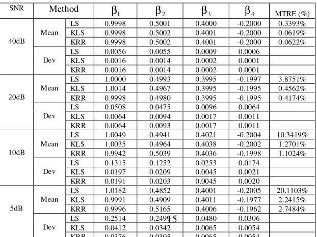
Table 2 Comparisons of the parameter estimates produced by the ordinary least squares algorithm and by the K-fold RSMM method, for the model given by (29)
SNR Method
1
β β2 β3 β4 MTRE (%)
LS 0.9998 0.5001 0.4000 -0.2000 0.3393% KLS 0.9998 0.5002 0.4001 -0.2000 0.0619% Mean
KRR 0.9998 0.5002 0.4001 -0.2000 0.0622% LS 0.0056 0.0055 0.0009 0.0006
KLS 0.0016 0.0014 0.0002 0.0001 40dB
Dev
KRR 0.0016 0.0014 0.0002 0.0001
LS 1.0000 0.4993 0.3995 -0.1997 3.8751% KLS 1.0014 0.4967 0.3995 -0.1995 0.4562% Mean
KRR 0.9998 0.4980 0.3995 -0.1995 0.4174% LS 0.0508 0.0475 0.0096 0.0064
KLS 0.0064 0.0094 0.0017 0.0011 20dB
Dev
KRR 0.0064 0.0093 0.0017 0.0011
LS 1.0049 0.4941 0.4021 -0.2004 10.3419% KLS 1.0035 0.4964 0.4038 -0.2002 1.2701% Mean
KRR 0.9942 0.5039 0.4036 -0.1998 1.1024% LS 0.1315 0.1252 0.0253 0.0174
KLS 0.0197 0.0209 0.0045 0.0021 10dB
Dev
KRR 0.0191 0.0203 0.0045 0.0020
LS 1.0182 0.4852 0.4001 -0.2005 20.1103% KLS 0.9991 0.4909 0.4011 -0.1977 2.2415% Mean
KRR 0.9996 0.5165 0.4006 -0.1962 2.7484% 5dB
• The variance of the parameter estimates produced by the K-fold ridge regression is less than that produced by the K-fold least squares method.
[image:16.612.138.449.538.771.2]4.2 Fruit fly modelling
The fruit fly insect dataset contains 1000 experimental data points for a wild type of fruit fly,
called Drosophila. The system input was the response of the photoreceptors (PR: mV), and the output
was the response of the large monopolar cells (LMCs, mV). The relationship between the input and
the output in the fruit fly experiment is complex, because in addition to the response from the
photoreceptors, several other factors may also affect the output response of the large monopolar cells.
The objective here was to find a model that reflects, as closely as possible, the relationship between
the response of the photoreceptors (the input) and the response of the large monopolar cells (the
output), to facilitate the analysis and understanding of the associate behaviour of this kind of insect.
The 1000 input-output data points, which are shown in Figure 1, were partitioned into two parts:
the training data set consisting of the first 800 points, and the test data set consisting of the remaining
200 points. A Volterra series model was employed to describe the input-output relationship of the fruit
fly data. The Volterra model is a special case of the linear-in-the-parameters form (3), where the
‘input’ (predictor) vector x(t)contains no lagged output y(t-k), with k≥1. The input vector x(t)for
the fruit fly data was chosen to bex(t)=[x1(t),x2(t),L ,x15(t)]T =[u(t−1),u(t−2),L ,
T t
u( −15)] , and
Fig. 1 The input and output signal for the fruit fly modelling problem.
∑∑
∑
= =
= − + − −
+
= 15
1 15
, 15
1
0 ( ) ( ) ( )
) (
i j i j i i
iu t i u t i u t j
t
y θ θ θ +e(t) (33)
A total of 136 candidate model terms were involved in the initial full model (33). A 10-fold random
subsampling and multifold modelling (RSMM) approach, along with the weighed average BIC given
by (20) where the weight coefficientα=0.5, was applied to the training dataset composed of the first
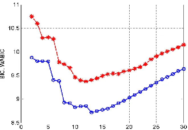
800 data points. For a comparison, the conventional orthogonal forward regression (OFR) algorithm,
along with the BIC given by (19), was also applied to the same training dataset. The BIC and WABIC,
shown in Figure 2, suggest that the model size for the OFR and RSMM produced models should be 13
and 12, respectively. The selected model terms for the two models are shown in Table 3, where
individual model terms are ranked in the order that they entered into the model.
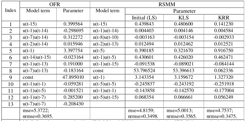
It can be seen from Table 3 that the performance of the RSMM produced model is slightly better
than that produced by using the traditional hold-out method, in the sense that the RSMM produced
model provides better predictive capability over the test dataset. More importantly, it can easily be
noted that by using the K-fold ridge regression, the very large initial least squares estimates of the 8th coefficient 53.7965 has been significantly reduced, without deteriorating the model’s generalisation
properties. This is important because, from the discussion of the previous section, the ridge penalised
model with shrinkage coefficients should be more robust. The model predicted output from the
RSMM produced model is shown in Figure 3. Note that Figure 3 illustrates the model predicted output
which is a much better indication of model performance than the one step ahead predicted output. The
latter is virtually coincident with the data set.
Table 3 Comparisons of the OFR and RSMM produced models for the fruit fly modeling problem
OFR RSMM
Parameter Index Model term Parameter Model term
Initial (LS) KLS KRR 1 u(t-15) 0.399564 u(t-15) 0.439843 0.480600 0.141230 2 u(t-1)u(t-14) -0.298695 u(t-1)u(t-14) 0.004403 0.004146 0.004584 3 u(t-7)u(t-14) 0.312272 u(t-8)u(t-10) -0.003163 -0.003154 -0.002933 4 u(t-2)u(t-14) 0.015946 u(t-2)u(t-13) 0.012494 0.012462 0.012521 5 u(t-1) 3.397754 u(t-5) 0.390185 0.321670 0.916750 6 u(t-14)u(t-15) -0.023164 u(t-1)u(t-5) 0.430601 0.426020 0.462471 7 u(t-1)u(t-13) 0.191000 u(t-1)u(t-15) -0.091538 -0.089021 -0.084144 8 u(t-7)u(t-13) -0.183164 const 53.796524 53.396613 0.062336 9 const 47.895010 u(t-1) 3.143354 3.159672 1.327320 10 u(t-1)u(t-1) -0.059281 u(t-5)u(t-5) -0.245837 -0.243192 -0.251918 11 u(t-1)u(t-5) -0.001521 u(t-1)u(t-1) -0.143858 -0.142570 -0.177004 12 u(t-1)u(t-7) 0.285200 u(t-5)u(t-15) 0.068354 0.066661 0.056249 13 u(t-7)u(t-7) -0.208430
mse=5.3722; nrmse=0.3695.
mse=4.8159; nrmse=0.3498.
mse=5.0013; nrmse=0.3565.
[image:19.612.121.485.448.772.2]mse=4.7537; nrmse=0.3475. LS: Ordinary least squares algorithm; KLS: LS based K-fold parameter estimation; KRR: Ridge regression based K-fold parameter estimation; The above MSE and NRMSE were calculated over the test dataset.
Fig. 3 A comparison of the model predicted output and the measurement for the fruit fly modelling problem. The thick solid line represents the measurement; the thick dashed line represents the model predicted output from the RSMM produced model; the thin solid line represents the model predicted output from the traditional hold-out method using the OFR algorithm.
5. Conclusions
The application of the new random subsampling and multifold modelling (RSMM) approach
involves two steps: model term selection and model parameter refinement. As in other random
sampling or bootstrapping methods, the information carried by a given data set can often be
sufficiently exploited for model identification by means of the proposed multifold random
subsampling approach. When the RSMM approach is applied to model structure selection, some kind
of multiple search procedures, over a number of partitioned datasets, are inevitably involved. It would
initially seem that the implementation of a multiple search is complex. Fortunately, however, the
introduction of the new multiple orthogonal search (MOS) algorithm enables the realisation of the
associated multiple search to be quite convenient.
For convenience of description and illustration, all the models involved in the given examples are
formed using polynomials. However, it should be stressed that the RSMM approach can also be
applied to any other parametric or non-parametric modelling problems, where the initial full models
can be written as a linear-in-the-parameters form.
The criterion used for model size determination in this study is a weighted average Bayesian
information criterion (WABIC), where a weight coefficient needs to be provided. However, how to
chose and optimise such a weight coefficient is still an open problem.
Acknowledgements
The authors gratefully acknowledge that this work was supported by the Engineering and Physical
Sciences Research Council (EPSRC), U.K. They are grateful to Dr M. Juusola, the University of
References
L.A. Aguirre and S. A. Billings, “Validating identified nonlinear models with chaotic dynamics”, Int. J. Bifurcation and Chaos, 4, pp.109-125, 1994.
L.A. Aguirre and S. A. Billings, “Retrieving dynamical invariants from chaotic data using narmax
models”, Int J Bifurcation and Chaos, 5, pp.449-474, 1995a.
L.A. Aguirre and S. A. Billings, “Improved structure selection for nonlinear models based on term
clustering”, Int. J. Control, 62, pp.569-587, 1995b.
H. Akaike, “A new look at the statistical model identification”, IEEE Transactions on Automatic Control, 19, pp. 716-723, 1974.
D. M. Allen, “The relationship between variable selection and data augmentation and a method for
prediction,” Technometrics, 16(1), pp. 125-127, 1974.
S. A. Billings and S. Chen, “Identification of nonlinear rational systems using a prediction error
estimation algorithm”, Int. J. Systems Sci., 20, pp.467-494, 1989.
S. A. Billings, S. Chen, and R. J. Backhouse, “The identification of linear and non-linear models of a
turbo charged diesel-engine”, Mechanical Systems and Signal Processing, 3(2), pp. 123-142, 1989a.
S. A. Billings, S. Chen, and M. J. Korenberg, “Identification of MIMO non-linear systems using a
forward-regression orthogonal estimator”, Int. J. Control, 49(6), pp. 2157-2189, 1989b.
S. A. Billings and Q. M. Zhu, “A structure detection algorithm for nonlinear dynamical rational
models”, Int. J. Control, 59(6), pp. 1439-1463, 1994.
S.A. Billings and H.L. Wei, ‘‘A new class of wavelet networks for nonlinear system identification’’,
IEEE Trans. Neural Networks, 16, pp. 862–874, 2005.
S. A. Billings and H. L. Wei, “An adaptive orthogonal search algorithm for model subset selection and
nonlinear system identification,” Int. J. Control, 2007 (in press).
L. Breiman, “Heuristics of instability and stabilization in model selection”, Ann. Statist., 24(6), pp.2350-2383, 1996.
L. Breiman and P. Spector, “Submodel selection and evaluation in regression—the X-random case”,
Int. Statist. Rev., 60(3), pp. 291-319, 1992.
M. Brown and C.J. Harris, Neurofuzzy Adaptive Modeling and Control. Hemel Hempstead: Prentice
Hall, 1994.
S. Chen, S. A. Billings and W. Luo, “Orthogonal least squares methods and their application to
nonlinear system identification”, Int. J. Control, 50(5), pp. 1873–1896, 1989.
S. Chen, P. M. Grant, and C. F. N. Cowan, “Orthogonal least-squares algorithm for training radial
basis function networks,” Proc. Inst. Elect. Eng.—Radar and Signal Process., pt. F, 139(6), pp. 378–384, 1992.
constructing radial basis function networks”, Int. J. Control, 64(5), pp. 829-837, 1996.
S. Chen, X. Hong, C. J. Harris, and P. M. Sharkey, “Sparse modeling using orthogonal regression with
PRESS statistic and regularization,” IEEE Trans. Sys. Man, Cyber. B, 34(2), pp. 898-911, 2004. V. Cherkassky and F. Mulier, Learning from Data. New York:Wiley, 1998.
M. V. Correa, L. A. Aguirre and E. M. A. M. Mendes, “Modelling chaotic dynamics with discrete
nonlinear rational models”, Int. J. Bifurcation and Chaos, 10(5), pp1019-1032, 2000.
P. A. Devijver and J. Kittler, Pattern Recognition: A Statistical Approach. London: Prentice-Hall, 1982.
B. Efron, “Estimating the error rate of a prediction rule: improvements on cross-validation”, J. Amer. Statist. Assoc., 78(382), pp316-331, 1983.
B. Efron and G. Gong, “A leisurely look at the bootstrap, the jackknife, and cross-validation”, Amer.
Statist., 37(1), pp.36-48, 1983.
B. Efron and R. J. Tibshirani, An Introduction to the Bootstrap. New York: Chapman & Hall, 1993. G. H. Golub, M. Heath, and G. Wahha, “Generalized cross-validation as a method for choosing a good
ridge parameter,” Technometrics, 21, pp. 215-223, 1979.
L. K. Hansen and J. Larsen, “Linear unlearning for cross-validation,” Adv. Comput. Math., 5, pp. 269– 280, 1996.
M. H. Hansen and B. Yu, “Model selection and the principle of minimum description length”, J. Amer. Statist. Assoc., 96(454), pp. 746–774, 2001.
C.J. Harris, X. Hong, and Q. Gan, Adaptive Modelling, Estimation and Fusion from Data : A Neurofuzzy Approach. Berlin ; London : Springer-Verlag, 2002.
A. E. Hoerl and R. W. Kennard, “Ridge regression: Biased estimation for nonorthogonal problems”,
Technometrics, 12(1), pp.55-67, 1970a.
A. E. Hoerl and R. W. Kennard, “Ridge regression: Application to nonorthogonal problems”,
Technometrics, 12(1), pp.69-82, 1970b.
A. E. Hoerl and R. W. Kennard, “Ridge regression iterative estimation of biasing parameter”,
Commun. Statist.—Theory Methods, 5(1), pp.77-88, 1976.
X. Hong, P.M. Sharkey and K. Warwick, ‘‘A robust non-linear identification algorithm using PRESS
statistic and forward regression’’, IEEE Trans. Neural Networks, 14(2), pp. 454–458, 2003a.
X. Hong, P.M. Sharkey and K. Warwick, ‘‘Automatic non-linear predictive model construction
algorithm using forward regression and the PRESS statistic’’, IEE Proceedings: Cont. Theory and
Applic., 150(3), pp. 245–254, 2003b.
X. Hong, C.J. Harris, S. Chen and P.M. Sharkey, ’’Robust non-linear system identification methods
using forward regression’’, IEEE Trans. on Systems, Man and Cybernetics – Part A, 33(4), pp.
514–523, 2003c.
X. Hong and X. Mitchell, “Backward elimination model construction for regression and classification
C. M. Hurvich and C. –L. Tsai, “Regression and time series model selection in small samples”,
Biometrika, 76(2), pp.297-307, 1989.
I. J. Leontaritis and S. A. Billings, “Input-output parametric models for non-linear systems, part I:
deterministic non-linear systems”, Int. J. Control, 41, pp. 303-344, 1985.
I. J. Leontaritis and S. A. Billings, “Experimental design and identifiability for nonlinear systems”, Int. J. Systems Sci., 18, pp.189-202, 1987.
G.P. Liu, Nonlinear Identification and Control: A Neural Network Approach. London: Springer, 2001.
L. Ljung, System Identification : Theory for the User. Englewood Cliffs : Prentice-Hall, 1987. L. Ljung, “Black-box models from input-output measurements”, in Proc. 18th IEEE Instrumentation
and Measurement Technology Conference (IMTC’2001), vol. 1, pp.138 - 146, Budapest, Hungary, May 21-23, 2001.
A. J. Miller, Subset Selection in Regression. London: Chapman and Hall, 1990.
G. Monari and G. Dreyfus, “Local overfitting control via leverages”, Neural Comput., 14(6), pp. 1481–1506, 2002.
D. C. Montgomery, E. A. Peck, and G. G. Vining, Introduction to Linear Regression Analysis (3rd Ed). New York: John Wiley & Sons, 2001.
R. Murray-Smith and T.A. Johansen, Multiple Model Approaches to Modeling and Control. London:
Taylor and Francis, 1997.
A. J. Myles, A. F. Murray, A. R. Wallace, J. Barnard, and G. Smith, “Estimating MLP generalisation
ability without a test set using fast, approximate leave-one-out cross-validation”, Neural Computing and Applications, 5(3), pp. 134-151, 1997.
R. K. Pearson, ‘‘Nonlinear input/output modelling’’, J. Process Control, 5, pp. 197–211, 1995.
R. K. Pearson, Discrete-Time Dynamic Models, New York: Oxford University Press, 1999. J. Rissanen, “Modelling by shortest data description”, Automatica, 14, pp. 465-471, 1978.
G. Schwarz, “Estimating the dimension of a model”, TheAnnals of Statistics, 6, pp. 461-464, 1978. J. Shao, “Linear-model selection by cross-validation”, J. Amer. Statist. Assoc., 88(422), pp. 486-494,
1993.
J. Shao, “An asymptotic theory for linear model selection”, Statistica Sinica, 7(2), pp. 221-242, 1997. J. Shao and D. Tu, The Jackknife and Bootstrap. New York: Springer-Verlag, 1995.
P. Stoica, P. Eykhoff, P. Janssen, and T. Soderstrom, “Model-structure selection by cross-validation”,
Int. J. Control, 43, pp. 1841-1878, 1986.
P. Stoica and Y. Selen, “Model-order selection: a review of information criterion rules”, IEEE Signal Proc.Magazine, 21, pp. 36-47, 2004.
M. Stone, “Cross-validatory choice and assessment of statistical predictions”, J. Royal Statist. Soc. Ser. B, 36(2), pp.111-147, 1974.
K. M. Tsang and W. L. Chan, “A search algorithm for the identification of multiple inputs nonlinear
2006.
N. V. Truong, L. Wang, and P. C. Young, “Non-linear system modelling based on non-parametric
identification and linear wavelet estimation of SDP models ”, Int. J. Control, 80(5), pp.774-788, 2007.
H. L. Wei, S.A. Billings and J. Liu, ‘‘Term and variable selection for nonlinear system identification’’,
Int. J. Control, 77, pp. 86–110, 2004.
H. L. Wei and S.A. Billings, ‘‘A unified wavelet-based modelling framework for nonlinear system
identification: the WANARX model structure’’, Int. J. Control, 77, pp. 351–366, 2004.
Q. M. Zhu and S. A. Billings, “Parameter-estimation for stochastic nonlinear rational models”, Int. J. Control, 57(2), pp. 309-333, 1993.
Q. M. Zhu and S. A. Billings, “Fast orthogonal identification of nonlinear stochastic models and radial