Integrated inventory management and supplier base reduction in a supply chain with multiple uncertainties

(1)

Other uses, including reproduction and distribution, or selling or

licensing copies, or posting to personal, institutional or third party

websites are prohibited.

In most cases authors are permitted to post their version of the

article (e.g. in Word or Tex form) to their personal website or

institutional repository. Authors requiring further information

regarding Elsevier’s archiving and manuscript policies are

encouraged to visit:

(2)

Production, Manufacturing and Logistics

Integrated inventory management and supplier base reduction

in a supply chain with multiple uncertainties

Dong-Ping Song

a,⇑

, Jing-Xin Dong

b

, Jingjing Xu

a,1

a_{School of Management, Plymouth University, Drake Circus, Plymouth PL4 8AA, UK} b

Business School, Newcastle University, Newcastle NE1 4SE, UK

a r t i c l e

i n f o

Article history:

Received 7 November 2012 Accepted 31 July 2013 Available online 8 August 2013

Keywords: Supply chain

Raw material procurement Production control Supplier base reduction Uncertainty

Integration

a b s t r a c t

This paper considers a manufacturing supply chain with multiple suppliers in the presence of multiple uncertainties such as uncertain material supplies, stochastic production times, and random customer demands. The system is subject to supply and production capacity constraints. We formulate the inte-grated inventory management policy for raw material procurement and production control using the sto-chastic dynamic programming approach. We then investigate the supplier base reduction strategies and the supplier differentiation issue under the integrated inventory management policy. The qualitative relationships between the supplier base size, the supplier capabilities and the total expected cost are established. Insights into differentiating the procurement decisions to different suppliers are provided. The model further enables us to quantitatively achieve the trade-off between the supplier base reduction and the supplier capability improvement, and quantify the supplier differentiation in terms of procure-ment decisions. Numerical examples are given to illustrate the results.

1. Introduction

Manufacturer-oriented supply chain systems are concerned with the effective management of the flow and storage of goods in the process from the procurement of raw materials from the suppliers to the delivery of finished goods to the customers. Here the flow refers to transporting materials and the storage refers to holding inventory. One of the key challenges in supply chain man-agement is how to appropriately tackle and respond to a variety of uncertain factors such as supply uncertainty and disruption (Lu,

Huang, & Shen, 2011; Snyder et al., 2012), imperfect production

or defective items (Pal, Sana, & Chaudhuri, 2013; Sana, 2010), unre-liable machines (Pal et al., 2013; Song & Sun, 1998); stochastic pro-cessing times (Buzacott & Shanthikumar, 1993; Song, 2013), and random demands (Masih-Tehrani, Xu, Kumara, & Li, 2011).

Traditionally, procurement policy about lot sizing decisions for raw materials was often separated from the production control systems so that the complexity and interplay of the functional areas like procurement, inventory, production and scheduling are decomposed and reduced. Such treatment is useful to simplify the management problem, and may be appropriate in situations with loose connections between functional areas. However, from

a systemic viewpoint, it may lead to sub-optimal solutions and the system may perform far away from the optimum. In the last two decades, much attention has been paid to the coordination be-tween procurement management and production management along the development of the supply chain management concept (e.g.Arshinder, Kanda, & Deshmukh, 2008; Goyal & Deshmukh, 1992; and the references therein). This paper will consider the optimal integrated procurement and production problem for a manufacturing supply chain with multiple suppliers in the pres-ence of multiple uncertainties such as uncertain material supplies, stochastic production times, and random customer demands. In the following, we review and classify the relevant literature into two groups. The ﬁrst group focuses on the sourcing (procurement) problems among multiple suppliers under supply uncertainty; and the second group focuses on the integrated inventory management for production systems subject to two or multiple types of uncertainties.

With respect to the ﬁrst group,Snyder et al. (2012)described several forms of supply uncertainty including: disruptions, yield uncertainty, capacity uncertainty, lead-time uncertainty, and input cost uncertainty; however, the boundaries among these forms are often blurry. Sourcing from multiple suppliers is an important strategy to deal with the supply uncertainty. The general sourcing (ordering) problem is to determine from how many and which suppliers to source the commodity (or raw material) and in what quantities in order to minimise total expected cost. A signiﬁcant number of studies have been conducted in this area in the last

http://dx.doi.org/10.1016/j.ejor.2013.07.044

⇑ Corresponding author. Tel.: +44 1752 585630; fax: +44 1752 585633. E-mail addresses:Dongping.song@plymouth.ac.uk(D.-P. Song),jingxin.dong@

ncl.ac.uk(J.-X. Dong),Jingjing.xu@plymouth.ac.uk(J. Xu).

1

Tel.: +44 1752 585630; fax: +44 1752 585633.

Contents lists available atScienceDirect

European Journal of Operational Research

(3)

two decades (cf. the review papers:Ho, Xu, & Dey, 2010; Minner,

2003; Qi, 2013; Thomas & Tyworth, 2006; Snyder et al., 2012).

More speciﬁcally, Lau and Zhao (1993) considered an inventory system with two suppliers subject to stochastic lead times and de-mands. They presented a procedure to determine the optimal or-der-splitting policy (i.e. the total order quantity, reorder point and proportion of split between two suppliers).Anupindi and

Akel-la (1993)studied a dual sourcing problem with stochastic demand

and supply uncertainty (e.g. random disruption and yield uncer-tainty). They proved that the optimal ordering policy has three ac-tion regions depending on the on-hand inventory level. Agrawal

and Nahmias (1997)developed a mathematical model to optimise

the number of suppliers with yield uncertainty. They assumed that the yield from an order is the placed order size multiplied by a nor-mal random variable, which implies that larger orders have higher yield variance. Such effect favours smaller orders from many sup-pliers. On the other hand, more suppliers incur additional ﬁxed costs associated with each supplier such as qualifying new suppli-ers, supplier development, and more logistics problems. Their model is able to ﬁnd the optimal number of suppliers that balances these two competing objectives. Berger, Gerstenfeld, and Zeng

(2004)examined the single versus multiple sourcing problem from

the risk management viewpoint and presented a decision-tree based optimisation model to evaluate the performance of the two procurement approaches. Here the risks refer to catastrophic events that affect many/all suppliers, and unique events that affect only a single supplier.Berger and Zeng (2006)extended the above decision-tree approach to considering unpredictable operations interruptions caused by all suppliers failing to satisfy the buyer’s demand so that the optimal size of the supply base can be deter-mined.Ruiz-Torres and Mahmoodi (2007)also utilised the decision tree approach to determine the optimal number of suppliers taking into account various levels of supplier failure probability and pos-sible procurement cost savings gained from using less reliable suppliers. Dada, Petruzzi, and Schwarz (2007) formulated a newsvendor model for the procurement decisions from multiple unreliable suppliers in which demand is stochastic and supply uncertainty can reﬂect disruptions, yield uncertainty, and capacity uncertainty. They showed that if a given supplier is not used, then no more expensive suppliers than this supplier should be used.

Federgruen and Yang (2008, 2009)examined the supplier selection

and diversiﬁcation issues in the similar inventory system to that of

Dada et al. (2007), but with different cost structures.

Burke, Carrillo, and Vakharia (2007)contrasted the preference

of single versus multiple supplier sourcing strategies in a single period, single product sourcing decisions under demand uncer-tainty. They showed that single sourcing strategy is preferred only when supplier capacities are large relative to the product demand and when the manufacturer does not obtain diversiﬁcation bene-ﬁts. In other cases, the multiple sourcing strategy is preferred.

Jo-kar and Sajadieh (2008)considered a multiple sourcing inventory

system with stochastic lead-times and constant demand under the reorder point-order quantity inventory control policy on a con-tinuous-review scheme. They presented a mathematical model that is able to determine the optimal number of identical suppliers and quantify the difference between multiple-sourcing and sole-sourcing strategies. Sarkar and Mohapatra (2009) formulated a model with a decision tree-like structure to determine the optimal size of supply base by considering the risks of supply disruption caused by different types of events. Masih-Tehrani et al. (2011)

showed that risk diversiﬁcation is preferred in a multi-manufac-turer-one-retailer system with stochastically dependent supply capacities, and indicated that if the retailer ignores the effect of dependent disruptions it would overestimate the ﬁll rate and tend to order more than the optimum.Lu et al. (2011)considered the optimal sourcing policy in a supply chain with product substitution

and dual sourcing under random supply failures.Mirahmadi,

Sa-beri, and Teimoury (2012)used a decision tree approach to

deter-mine the optimal number of suppliers taking into account the supply risk and the associated costs (e.g. cost of supplier develop-ment, missing discount in volume, loss due to supply postpone-ment). Silbermayr and Minner (2012) presented a semi-Markov decision process for the optimal sourcing problem with multiple suppliers in which demands, lead times and supplier availability are all stochastic. They showed that the optimal sourcing strategy (depending on the on-hand inventory, the outstanding orders and the supplier availability statuses) is rather complex.Pal, Sana, and

Chaudhuri (2012a)addressed a multi-echelon suppler chain with

two suppliers in which the main supplier may face supply disrup-tion and the secondary supplier is reliable but more expensive, and the manufacturer may produce defective items.Arts and

Kiesmul-ler (2013)studied a serial two-echelon periodic-review inventory

system with two supply modes, and showed that dual-sourcing can lead to signiﬁcant cost savings in cases with high demand uncertainty, high backlogging cost or long lead times.

With regard to the second group that addresses production-inventory control in the presence of uncertainties, a rich literature existed. The earliest relevant research could date back to early 1960s, e.g.Clark and Scarf (1960)studied the multi-stage or mul-ti-echelon inventory systems with random demand and determin-istic lead-time. When two or more types of uncertainties are modelled, the optimal production and inventory policies are often addressed within a single-stage, two-stage, or three-stage context. In the following, we mainly select the relevant literature consider-ing two or multiple uncertainties with an emphasis on stochastic lead times.

Hadley and Whitin (1963)addressed a single-stage inventory

management problem and identiﬁed the optimal inventory control policies for some special cases with restrictive assumptions, e.g. or-ders do not cross each other and they are independent. Zipkin

(1986) characterized the distributions of inventory level and

inventory position in continuous-time single-stage models with stochastic demand and lead times.Bassok and Akella (1991) inves-tigated the optimal production level and order quantity with sup-ply quality and demand uncertainty. Song and Zipkin (1996)

studied a single-stage system with random demand and Markov modulated lead-times, and were able to characterise the optimal inventory control policy. Berman and Kim (2001)examined the optimal dynamic ordering problem in a two-stage supply chain with Erlang distributed lead-times, exponential service times and Poisson customer arrivals. They showed the optimal ordering pol-icy has a monotonic threshold structure.Berman and Kim (2004)

extended the above model to including revenue generated upon the service considering both exponential and Erlang lead times.

He, Jewkes, and Buzacott (2002)considered a two-echelon

make-to-order system with Poisson demand, exponential processing times, and zero lead times for ordering raw materials, and explored the structure of the optimal replenishment policy. Yang (2004)

studies a periodic-review production control problem where both the raw material supply and product demand are exogenous and random. He was able to establish the partial characterisation of the optimal policies under both strict convex and linear raw mate-rial purchasing/selling costs.Simchi-Levi and Zhao (2005) investi-gated the safety stock positioning problem in multistage supply chains with tree network structure with stochastic demands and lead times, in which a continuous-time base-stock policy is used in each stage to control its inventory. Mukhopadhyay and Ma

(2009)considered the optimal procurement and production

(4)

applied the base-stock policy to single and multistage inventory systems with stochastic lead times and provided a method to determine base-stock levels and to compute the costs of a given base-stock policy.Pal, Sana, and Chaudhuri (2012b)presented an analytical method to optimise the production rate and raw mate-rial order size in a three-layer supply chain subject to imperfect quality raw materials, unreliable machine and defective product reworking.Sana (2012)presented a collaborative inventory model for a three-layer supply chain subject to defective items in produc-tion and transportaproduc-tion, and determined the optimal producproduc-tion rate, order quantity, and number of shipments.Song (2013) exam-ined the optimal and sub-optimal integrated ordering and produc-tion policies in several stochastic supply chain systems.

From the above literature review, it can be observed that the ﬁrst group of studies mainly focused on the sourcing strategies from multiple suppliers with supply uncertainty and did not explicitly consider the production decisions and processing uncer-tainty; whereas the second group mainly focused on production and inventory management in supply chain systems with two or more types of uncertainties (e.g. demand and lead time) but with a single supplier. From the supply chain integration perspective, manufacturers intend to reduce supplier base to a manageable size so that a closer relationship with suppliers can be established (

Gof-ﬁn, Szwejczewski, & New, 1997). The manufacturer may gain

ben-efits of cheaper unit costs and more reliable delivery performance from suppliers, whereas the suppliers can gain benefits of larger and more stable demands. On the other hand, from the supply uncertainty perspective, manufacturers intend to source from mul-tiple suppliers to buffer against the supply uncertainty. It is clear that there is a trade-off between reducing the impact of uncertain-ties (by having a larger number of suppliers) and reducing the pro-curement costs associated with each supplier (by having a smaller size of supplier base and closer relationship). However, it is be-lieved that the supplier base reduction strategy is related to the procurement policy, the production policy and other stochastic fac-tors in the manufacturing supply chain. Therefore, there is a need to investigate the integrated material procurement and production control policy and supplier base reduction strategies in manufac-turer-oriented supply chains with multiple types of uncertainties. This paper considers a manufacturing supply chain with multi-ple suppliers in the presence of multimulti-ple uncertainties with an emphasis on integrated inventory management, supplier base reduction and supplier differentiation. The objective function is the expected total cost consisting of raw material inventory cost, raw material ordering processing costs, finished goods inventory cost, and customer demand backlogging cost. The integrated inventory management problem concerns the joint decision-making including when and in what quantities to procure raw materials from which suppliers, and when to produce finished goods. The supplier base reduction strategy concerns the trade-off between reducing the number of suppliers and requiring the higher capabilities of suppliers (such as higher shipping capacity, shorter lead-time, more reliable delivery, and lower order pro-cessing cost). The supplier differentiation concerns the difference and relationship of the procurement decisions between different suppliers. Here the supplier differentiation is slightly different from the concept of order splitting in the literature, which refers to dividing a large order into smaller orders among multiple sup-pliers in order to reduce the effective replenishment lead-time

(Thomas & Tyworth, 2006). Speciﬁc research objectives of this

study include:

formulate the integrated inventory management problem for raw material procurement and production control in a manu-facturing supply chain with multiple suppliers and multiple types of uncertainties, and seek the optimal policy;

establish the qualitative relationship between the expected total cost and the supplier base size, and the supplier capabilities (such as the suppliers’ delivery capacity, the suppliers’ delivery reliabil-ity); and establish the qualitative relationship of the optimal pro-curement decisions between different suppliers;

evaluate the quantitative impacts of the supplier based reduc-tion strategies, i.e. supplier base reducreduc-tion combined with sup-plier capability improvement, on the system performance so that a trade-off can be achieved; and also quantify the supplier differentiation.

The rest of this paper is organised as follows. In the next section, the system under consideration is described and formulated math-ematically. The optimal integrated policy for raw material procure-ment and production control is presented using the stochastic dynamic programming approach. In Section3, the qualitative rela-tionships between the expected total cost and the supplier base size, and the supplier capabilities are established. In Section4, sev-eral supplier base reduction strategies are presented and the trade-off effect is discussed. In Section5, the supplier differentiation is-sue is addressed and insights are provided. In Section6, we extend the model by relaxing a key assumption. In Section7, a range of numerical scenarios are analysed to verify and illustrate the ana-lytical results. The best trade-off between the supplier base reduc-tion and the supplier capability improvement is achieved. The structural characteristics of the optimal procurement and produc-tion policies are explored and discussed. Finally, the main contri-butions and the managerial insights are concluded in Section8.

2. Optimal integrated procurement and production policy

The supply chain under consideration consists of three levels of entities, i.e. suppliers, manufacturer and customers. It is assumed there is sufficient warehouse capacity to store raw material (RM) and finished goods (FG). There areNsuppliers that are contracted with the manufacturer to supply the raw materials. The manufac-turer may place different sizes of orders to different suppliers to buffer against the uncertainty in RM supply. The quantity of an or-der to supplieri, denoted asqi, is a decision variable that is con-strained by the maximum order quantity Qi, which represents the delivery capacity of supplieri. The RM replenishment lead-time from supplierito the manufacturer is a random variable following an exponential distribution with the mean 1/ki. The lead-time is as-sumed to be independent on actual order quantity, which may be justified by the fact that the dispatching equipment usually can de-liver up to the quantityQiin a single trip. It is assumed that one unit of RM is required to produce one unit of product. The manu-facturer produces one product at a time and the processing time is exponentially distributed with the mean 1/u. Physically,u repre-sents the production (or service) rate (e.g.Veatch & Wein, 1994). It is a control variable that takes 0 orU, which represents an action ‘‘not produce’’ or ‘‘produce at a speedU’’, respectively (the model can be extended easily to the case of allowingutaking more values between 0 andU, but the results remain the same). Customer de-mands arrive one at a time following a Poisson process with arriv-ing raten. A demand is satisfied immediately if there are FGs stored in the warehouse; otherwise unmet demands are backlogged.

(5)

costs since more time and effort has been committed. However, two types of costs associated with RM procurement and delivery processes will be incurred to the manufacturer. The first is a fixed cost which is charged whenever there exists a non-zero outstand-ing order regardless of the order size. The second is a variable cost which is proportional to the order size of the outstanding order. The assumption that the outstanding order can be modified at any time before arrival together with the exponential lead-time assumption implies that there is no more than one outstanding or-der at any time for each supplier. The assumption of at most one outstanding order at any time was first introduced inHadley and

Whitin (1963), and often used in other literature, e.g. Berman

and Kim (2001, 2004) and Kim (2005). The exponential order

replenishment lead-time was also assumed in Berman and Kim

(2004), Kim (2005), and Silbermayr and Minner (2012). The

expo-nential manufacturing time has been adopted in more literature,

e.g.Ching, Chan, and Zhou (1997), Feng and Yan (2000), Feng and

Xiao (2002), He et al. (2002), Song and Sun (1998) and Veatch

and Wein (1992, 1994). The Poisson demand arrival is one of the

most common assumptions in the related literature (e.g.Buzacott

& Shanthikumar, 1993). Note that the assumption of adjustable

outstanding orders is rather restrictive from the practical perspec-tive. We will relax this assumption in the late sections and inves-tigate the impact of such assumption on the main results.

The decisions of order quantities for RMs are constrained by the maximum order quantity Qi; while the production rate is con-strained by the capacity Uand the availability of raw materials.

Letx1(t) denote the on-hand inventory level of RMs at timetand

x2(t) denote the on-hand inventory level of FGs at timet. Here

x2(t) could be negative, which represents the number of back-logged demands. The manufacturer needs to make two types of decisions: the production rateu2{0,U} and the RM order

quanti-tiesqifori2[1,N] subject to 06qi6Qi. Whenqi= 0, it implies that

supplier i is not selected to supply raw materials at the current decision-making epoch. Deﬁne the control decision vector

u:¼(u,q1,q2,. . .,qN). From the assumption that the outstanding orders are adjustable before reaching the manufacturer, the out-standing orders can be treated as control variables. Therefore, the system state can be described by a vectorx= (x1,x2), which repre-sents the inventory levels of RMs and FGs. It should be pointed out that when the adjustable outstanding order assumption is relaxed, the system state must include the status of the outstanding orders to all suppliers (see Section6).

The system state space is denoted byX= {x= (x1,x2)jx12Z+_and x22Z}. The evolution of the system state is driven by three types of events: the arrival of raw materials from one of the suppliers, the completion of production of a ﬁnished product, and the arrival of a customer demand. In other words, the system state will not change unless one of the above events occurs. It should be pointed out that due to the memoryless properties of the Poisson process and the exponential distribution, the remaining time for a shipment, a production and for a demand whose arrival completion was inter-rupted by an event still follows the same exponential distribution.

We focus on state-feedback policies, in which the decisions are triggered by the system state changes. Therefore, u(t) should be understood as u(x(t)), wherex(t) represents the current system state at time t. Define an admissible control set X= {u= (u(x), q1(x),q2(x),. . .,qN(x))ju(x)2{0,U} if x1> 0, u= 0 if x160; 06 qi(x)6Qi for i= 1, 2,. . .,N}. To simplify the narrative, we often simplifyu(x) andqi(x) asuandqiby omitting the system state in the rest of the paper. The integrated inventory management problem is to find the optimal joint policy u2Xby minimising the infinite horizon expected discounted cost.

Jðx0Þ ¼min

u E

Z 1

0

ebt_G_ð_x_ð_t_Þ_;_u_ð_t_ÞÞ_dt_j_x_ð₀_{Þ ¼}_x 0

ð1Þ

where 0 <b< 1 is a discount factor,x0is the initial system state, and G(x(t),u(t)) represents the raw material holding costs, finished goods inventory costs, customer demand backlog costs, production costs, raw material fixed ordering costs, raw material variable ordering costs, which may be defined as

GðxðtÞ;uðtÞÞ ¼gðxðtÞÞ þcpuðtÞ þ XN

i¼1

cfiIfqiðtÞ>0g þcviqiðtÞ

ð2Þ

whereI{.} is an indicator function, which takes 1 if the condition is true, takes 0 otherwise; cf_i P0 and cv_i P0 are cost coefficients representing fixed ordering costs and variable ordering costs respectively; cp represents the production cost coefficient. Here the ordering costs (fixed and variable) are charged as long as the orders have been placed but have not reached the manufacturer. This can be interpreted as the aggregated costs including order handling, shipping and in-transition inventory costs. In (2), g(x(t)) represents the raw material inventory holding costs, finished goods holding costs and demand backlogging cost, defined by

gðxðtÞÞ ¼c1x1ðtÞ þcþ2x

þ

2ðtÞ þc

2x

2ðtÞ ð3Þ

where c1 and cþ

2 are holding cost for raw material and ﬁnished goods respectively; c

2 is the backlog cost; and xþ

2ðtÞ:¼maxf0;x2ðtÞg, andx2ðtÞ:¼maxf0;x2ðtÞg.

The problem in (1) is a continuous time Markov decision prob-lem, which can be transformed into an equivalent discrete-time Markov chain problem by using the uniformisation technique (

Pu-terman, 1994; Song, 2013), e.g. let

v

¼nþUþPN1ki be the

uni-form transition rate. The details of the transuni-forming process are given in the Appendix and the similar formulation process can be referred to Song (2013). From the stochastic dynamic program-ming theory, we have the following results.

Proposition 1. The optimal integrated procurement and production

policy u_ð_x_Þ_;_q

1ðxÞ;q2ðxÞ;. . .;qNðxÞ

is given by:

q

iðxÞ ¼arg min cviqiþIfqi>0g c f

iþkiJðx1þqi;x2Þj06qi6Qi

n o

; fori

¼1;2;. . .;N

ð4Þ

u_ð_x_{Þ ¼} U cpþJðx11;x2þ1Þ<Jðx1;x2Þ;x1>0

0 othewise

ð5Þ

Physically, the quantitycv

iqiþcfiþkiðJðx1þqi;x2Þ Jðx1;x2ÞÞ is the additional cost incurred when an order with non-zero sizeqi is placed to suppliericompared to no order is placed to supplier

i. On the other hand, the quantityU(cp+J(x11,x2+ 1)J(x1,x2))

is the additional cost incurred when the manufacturer is producing at the speedUcompared to producing nothing. Therefore, the man-ufacturer should produce nothing if the additional cost is non-negative.

The optimal policy given inProposition 1is implicit. To imple-ment it in reality, we need to know the explicit optimal cost func-tion J(x) or the additional cost incurred for the procurement decisions and the production decisions at any system state. From

theAppendix, we have the following result.

Proposition 2. Let J0(x) = 0 for anyx2X, Jk(x) = +1forxRX and

kP0, and

Jkþ1ðxÞ ¼ ðbþ

v

Þ

1

gðxÞ þnJkðx1;x21Þ þUminfcpþJkðx11;x2

þ1Þ;JkðxÞg þ XN

i¼1

min cviqiþIfqi>0g cfiþkiJkðx1þqi;x2Þj06qi6Qi

n o#

(6)

forkP0 andx2X, whereJk(x) is thek-stage cost function for state

x, then

lim

k!þ1JkðxÞ ¼JðxÞ; forx2X ð7Þ

whereJ(x) is deﬁned in (1).

The convergence of thek-stage policy and cost function to the inﬁnite-horizon optimal policy and cost again follows from the fact that a ﬁnite number of controls are taken at each state (Bertsekas,

1976, Chapter 6, Propositions 8–12). Based onProposition 2, the

value iteration algorithm below can be used to approximate the optimal cost function.

The value iteration algorithm

Specify the maximum iteration numberKand the error allow-ance

e

which is a small positive number. Letkdenote the iteration number,

Step 0: Setk= 0 andJ0(x)0 for anyx2X; and deﬁneJk(x):¼+1

forxRXandkP0.

Step 1: ComputeJk+1(x) using Eq.(6).

Step 2: Calculated= max{jJk+1(x)Jk(x)jforx2X}.

Step 3: Ifd<

e

ork>Kgo to Step 4; otherwise replacekbyk+ 1

and go to Step 1.

Step 4: Output Jk+1(x) and the resulting policy (u(x),q1(x),q2

(x),. . .,qN(x)) realising the minimisation of the right-hand-side of(6). Terminate the algorithm.

3. Impact of supplier base reduction and supplier capability improvement

We deﬁne the supplier capability as its ability to provide higher service level (e.g. higher delivery capacity, faster delivery, more reliable delivery) or lower ordering costs (e.g. cheaper ﬁxed or var-iable order processing costs). This section investigates the impacts of the supplier base reduction and the supplier capability improve-ment on the total expected cost.

Proposition 3. (i) J(x) is decreasing as ki increases; (ii) J(x) is

decreasing as U increases.

Proof. For assertion (i), letJ0₍_x_{) denote the expected discounted}

cost withk0

i, which is greater thanki. Deﬁne the uniform transition rate

v

¼nþUþPn1k

0

i for both caseskiandk 0

i. We want to prove J(x)PJ0₍_x_{) by the induction approach. For any}_x_{, it is obvious that} J0ðxÞ 0PJ00ðxÞ 0. Suppose JkðxÞPJ0kðxÞ. We want to show J_kþ₁ðxÞPJ0

kþ1ðxÞ. FromProposition 2,

Jkþ1ðxÞ ¼ ðbþ

vÞ

1

gðxÞ þnJkðx1;x21Þ þUminfcpþJkðx11;

x2þ1Þ;JkðxÞg þ

Xn

1 k0iki

JkðxÞ þX n

1

min cviqiþIfqi>0g

cf

iþkiJkðx1þqi;x2Þj06qi6Qi oi

ð8Þ

and

J0

kþ1ðxÞ ¼ ðbþ

v

Þ

1

gðxÞ þnJ0

kðx1;x21Þ þUmincp

þJ0

kðx11;x2þ1Þ;J0kðxÞ

þX

n

1

min cviqiþIfqi>0g

cfiþk 0 iJ

0

kðx1þqi;x2Þj06qi6Qi oi

ð9Þ

Suppose that arg min cv

iqiþIfqi>0g c f

iþkiJkðx1þqi;x2Þ n

j06_q

i6Qig ¼qi >0; otherwise it is straightforward from the induction hypotheses. This implies that

cviq i þ c

f

iþkiJkðx1þqi;x2Þ

<kiJkðxÞ

Namely,

k0iki

JkðxÞ> k 0 iki

cviqi þ c

f

i þkiJkx1þqi;x2

.

ki;

ð10Þ

It follows,

min cv

iqiþIfqi>0g c f

iþkiJkðx1þqi;x2Þj06qi6Qi

n o

þ k0 iki

_J

kðxÞ

¼ cviqiþ c f

iþkiJkx1þqi;x2

þ k0iki

JkðxÞ

> cv iqiþ c

f

iþkiJkx1þqi;x2

þ k0 iki

cv iqiþ c

f

iþkiJkx1þqi;x2

=ki;

¼k0i cviqiþ c f

iþkiJkx1þqi;x2

=ki;

¼k0 i cviqiþc

f i

=kiþk0

iJkx1þqi;x2;

>cviqiþc f iþk

0

iJkx1þqi;x2

;

>cviq iþc

f iþk

0 iJ

0

kx1þqi;x2 ;

>min cviqiþIfqi>0g cfiþkiJ 0

kðx1þqi;x2Þj06qi6Qi

n o

By the induction hypotheses, we haveJkþ1ðxÞPJ0kþ1ðxÞ. By

Proposi-tion 2, we haveJ(x)PJ0₍_x_{). Hence, assertion (i) is true. Assertion (ii)}

can be proved similarly. This completes the proof. h

Note that the material lead-time from supplier i follows an exponential distribution with average 1/kiand variance 1/k2i. This implies that, askiincreases, the average delivery time and its var-iability are reduced. Therefore, Proposition 3(i) is in agreement with the intuition that shorter expected material lead time and more reliable delivery is beneﬁcial to the manufacturer since the manufacturer could maintain lower level of raw material invento-ries to buffer against the uncertainty in material supply.

Proposi-tion 3(ii) can be similarly interpreted.

Remark 1. (i) J(x) is decreasing as N increases; (ii) J(x) is

decreasing as Qi increases; (iii) J(x) is increasing as cfi or cvi increases.

The ﬁrst two assertions inRemark 1are intuitively true from the relaxation argument that an optimal solution of a relaxed prob-lem cannot be worse. The third assertion is intuitive and can be shown fromProposition 2by the induction approach. Physically, assertion (i) indicates that the manufacturer can reduce the cost if the supplier base increases; while assertions (ii) and (iii) imply that having a supplier with higher delivery capacities or lower or-der processing costs is more beneﬁcial to the manufacturer.

4. Supplier base reduction strategies

From the supply chain management perspective, the manufac-turer may want to establish a closer relationship with suppliers through supplier management strategies, e.g. the supplier base reduction. Reducing supplier base implies that the selected suppli-ers will have more sales. In return, the manufacturer often requires or expects that those selected suppliers can provide higher service level or lower ordering costs.

According to the supplier’s capability improvement, it gives rise to three types of supplier base reduction strategies:

the manufacturer reduces its supplier base size, whereas the selected suppliers provide higher delivery capacity. This strat-egy is called supplier base reduction with higher delivery capac-ity (SBR-HDC);

(7)

the manufacturer reduces its supplier base size, whereas the selected suppliers offer more efficient order processing service, which leads to lower fixed ordering costs. This strategy is called supplier base reduction with lower fixed ordering cost (SBR-LFC).

Proposition 3(i) andRemark 1indicate that the supplier base

reduction and the supplier capability improvement have opposite impacts on the total cost. A trade-off exists. However, it is not intu-itive to identify the trade-off point because of their interaction and the dependency on the integrated procurement and production pol-icy. Note that the supplier base size and the supplier capability are changing simultaneously under each of the supplier base reduction strategies, identifying the trade-off point is essentially a one-dimen-sional optimisation problem. This is not difﬁcult to solve, e.g. using the value iteration method iteratively. In terms of the location of the trade-off point, we have the following conjecture.

Conjecture 1. Under one of the above supplier base reduction

strategies, the system performance has a U-shape with respect to the degree of each supplier base reduction strategy. Here the degree of supplier base reduction strategy measures how far the supplier base has been reduced.

InConjecture 1, U-shape is used in a broad sense. It includes the

cases of monotonic increasing or monotonic decreasing situations. If the system performance is monotonically increasing as the size of supplier base decreases, then the best supplier base reduction strategy is to use a single supplier. On the other hand, if the system performance is monotonically decreasing as the size of supplier base decreases, then the best supplier base reduction strategy is to have the maximum number of available suppliers. We will ver-ify this conjecture in the numerical experiment section.

It should be pointed out that in real cases extra costs may be in-curred or intangible beneﬁt may be generated in the processes of supply base reduction and supply capability improvement, which may affect the trade-off point in the supplier base reduction strat-egies. However, this is a complicated and case-dependent issue, which deserves further research.

5. Supplier differentiation

Another important supplier management strategy is to differen-tiate suppliers when they have different supply capabilities. In other words, when suppliers have different delivery parameters (represented byQi; cfi; cvi, andkiin our model), the manufacturer should differentiate its procurement decisions in order to achieve the best performance.

Proposition 4. Under the optimal integrated procurement and

production policy u_ð_x_Þ_;_q

1ðxÞ;q2ðxÞ;. . .;qNðxÞ

given inProposition

1, we have the following relationships of the procurement decisions

between different suppliers:

(i)If Ql<Qjand all other parameters are the same for suppliers l

and j, then q

l(x)6qj(x).

(ii)If cf_l>cf_j and all other parameters are the same for suppliers l

and j, then q

lðxÞ6qjðxÞ, and if qlðxÞ>0, then qjðxÞ ¼qlðxÞ. (iii)If cv

l >cvj and all other parameters are the same for suppliers l

and j, then q

l(x)6qj(x).

(iv)Ifkl<kjand all other parameters are the same for suppliers l

and j, then q

l(x)6qj(x).

Proof.FromProposition 1, we know that the optimal order

quan-tity is determined by

q

iðxÞ ¼arg min cviqiþIfqi>0g c f

iþkiJðx1þqi;x2Þj06qi6Qi

n o

;

fori¼1;2;. . .;N

Assertion (i) is obvious from the above equation. To show the rest of assertions, we introduce the following two types of discrete func-tions to simplify the narrative,

fiðx;nÞ:¼civnþIfn>0g c f

i ð11Þ

hiðx;nÞ:¼kiJðx1þn;x2Þ ð12Þ It implies that

q

iðxÞ ¼arg minffiðx;nÞ þhiðx;nÞj06n6Qig ð13Þ

For assertion (ii): becauseq

iðxÞare non-negative integers, we only need to show ifq

lðxÞ>0, thenqjðxÞ ¼qlðxÞ. SupposeqlðxÞ ¼m>0. It follows,fl(x,m) +hl(x,m)6fl(x,n) +hl(x,n) for 06n6Qi. That is,

cvl mþc f

lþhlðx;mÞ6hlðx;0Þ ð14Þ

cvl mþc f

lþhlðx;mÞ6cvl nþc f

l þhlðx;nÞ for 0<n6Ql ð15Þ

Note thatcf l >c

f

j; cvl ¼cvj; Ql¼Qj, andhl(x,n) =hj(x,n). The above two equations lead to,

fjðx;mÞ þhjðx;mÞ6fjðx;nÞ þhjðx;nÞ for 06n6Qj ð16Þ

It follows,q

jðxÞ ¼m¼qlðxÞ. Thus, assertion (ii) is true. For assertion (iii): we want to show that if q

lðxÞ>0, then

q

jðxÞPqlðxÞ. SupposeqlðxÞ ¼m>0. We have the same Eqs.(14) and (15). Note thatcv_l >c_jv; cf_l ¼cf_j; Ql¼Qj, andhl(x,n) =hj(x,n). It follows,

cvj mþc f

jþhjðx;mÞ6hjðx;0Þ ð17Þ

cvj mþc f

jþhjðx;mÞ6cvj nþc f

jþhjðx; nÞ for 0<n6m ð18Þ

That yields,q

jðxÞPm¼qlðxÞ. Therefore, assertion (iii) is true. For assertion (iv), it can be similarly proved. This completes the proof.

h

Physically, Proposition 4 states that larger orders should be placed to the suppliers with higher supply capabilities, which is in agreement in intuition. In particular,Proposition 4(ii) provides a further interesting insight that if two suppliers only differ in the fixed ordering cost, the optimal non-zero procurement deci-sions to the supplier with higher fixed ordering cost should be the same as that to the supplier with lower fixed ordering cost. The interpretation is that if the optimal decision at a system state

x is to place a non-zero order to the supplier with higher ﬁxed ordering cost (which implies that this procurement decision can offset the incurred ﬁxed ordering costs to both suppliers), then the optimal order size to these two suppliers at the system state

xwill not be affected by the difference of their ﬁxed ordering costs. The results inProposition 4are qualitative. However, our model is able to quantify the differences of the optimal procurement deci-sions for different suppliers, which will be illustrated in the numer-ical example section.

6. Extension to the case with non-adjustable outstanding orders

(8)

Since the outstanding orders are not allowed to change once they are issued, the manufacturer’s new ordering decisions should depend on not only the inventory-on-hand of raw materials and ﬁnished goods, but also the inventory-in-transition, i.e. the out-standing orders (Silbermayr & Minner, 2012). The system state space can now be described byX:¼{(x,y)jx= (x1,x2) s.t.x12Z+ andx22Z;y= (y1,y2,. . .,yN) s.t. 06y_i6Q_ifori= 1, 2,. . .,N}. The manufacturer needs to make two types of decisions at any state (x,y): the production rateu2{0,U}, and the raw material order quantities 06q_i6Q_iI{y_i= 0} for i= 1, 2,. . .,N. Clearly, if yi> 0 for i= 1, 2,. . .,N, which represents the situation that there are non-zero outstanding orders to every supplier, then no new orders can be placed to any supplier. The admissible control set is deﬁned as X= {u= (u(x,y),q1(x,y),q2(x,y),. . .,qN(x,y))ju(x, y)2{0,U} if x1> 0,u= 0 ifx16_{0; 0}6_q_i₍_x₎6_Q_i_I{y_i_{= 0} for}_i_{= 1, 2,}_{. . .}_,_{N}. To}

simplify the narrative, we simplifyu(x) andqi(x) asuandqiby omitting the system state and letq:¼(q1,q2,. . .,qN).

The cost functionJ(x,y) can be deﬁned similar to (1) by replac-ingG(x,u) withG(x,y,u), which represents the incurred unit-time cost at state (x,y) taking control actionu,

Gðx;y;uÞ ¼gðxÞ þcpuþ XN

i¼1

cfiIfyiþqi>0g þcvi ðyiþqiÞ

ð19Þ

Following the uniformization technique (deﬁne

v

¼nþUþPN₁ki) and the stochastic dynamic programming theory, the Bellman opti-mality equation is given as follows

Jðx;yÞ ¼ ðbþ

v

Þ1 min

u2f0;Ug;06qi6QiIfyi¼0g h

Gðx;y;uÞ þnJðx1;x2

1;yþqÞ þuJðx11;x2þ1;yþqÞ þ

XN

i¼1 kiJðx1

þyiþqi;x2;y1þq1;. . .;yi1þqi1;0;yiþ1 þqiþ1;. . .;yNþqNg þ ðUuÞJðx;yþqÞ

i

ð20Þ

To simplify the narrative, let (x1+yi+qi, x2, y+qnyi+qi):¼ (x1+yi+qi, x2, y1+q1,. . .,yi1+qi1, 0, yi+1+qi+1,. . .,yN+qN,). The above equation can be simpliﬁed as,

Jðx;yÞ ¼ ðbþ

vÞ

1 gðxÞ þ min

06qi6QiIfyi¼0g

nJðx1;x21;yþqÞ

þUminfcpþJðx11;x2þ1;yþqÞ;Jðx;yþqÞg

þX

N

i¼1 cf

iIfyiþqi>0g þcvi

ðyiþqiÞ þkiJðx1þyiþqi;x2;yþqnyiþqiÞÞ

ð21Þ

From(21), the optimal integrated procurement and production pol-icy (u⁄₍_x_,_y_),_q⁄₍_x_,_y_{)) for the case with non-adjustable outstanding}

orders can be given by:

q ðx;yÞ ¼ q

1ðx;yÞ;q

2ðx;yÞ;. . .;q

Nðx;yÞ

¼arg min

06qi6QiIfyi¼0gfnJðx1;x21;yþqÞ þUminfcpþJðx11;x2þ1;yþqÞ;Jðx;yþqÞg

þX N

i¼1

cf

iIfyiþqi>0g þcvi ðyiþqiÞ þkiJðx1þyiþqi;x2;yþqnyiþqiÞ

)

ð22Þ

u_ð_x_;_y_{Þ ¼} U cpþJðx11;x2þ1;yþq _Þ_<_J_ð_x

1;x2;yþqÞ;x1>0 0 othewise

ð23Þ

Apart from the system state, another important difference between

(22) and (23)and(4) and (5)is that the procurement decisions are

coupled and they are also coupled with the production decision

in (22) and (23), whereas they are de-coupled in Proposition 1.

Nevertheless, from(21), it is clear that the value function approxi-mation procedure inProposition 2can be similarly applied to the case with non-adjustable outstanding orders.

It is straightforward to extend the results inRemark 1to the case with non-adjustable outstanding orders. However, it is chal-lenging to establish the property inProposition 3mathematically due to the coupled relationships of the procurement and produc-tion decisions. However, we will use numerical examples to illus-trate that the results inProposition 3andProposition 4can carry over to the case with non-adjustable outstanding orders. In addi-tion, a full factorial experiment will be conducted to investigate the impact of various factors (including the parameters represent-ing three different types of uncertainties) and their interactions on the system performance.

7. Numerical examples

This section consists of four sub-sections. In Section 7.1, we numerically illustrate the analytical results about the impacts of the supplier base size and the supplier capabilities on the system performance. In Section7.2, the trade-off relationships under the supplier base reduction strategies (inConjecture 1) are verified using a range of scenarios. The best trade-off point under each sup-plier base reduction strategy is identified. In Section7.3, we illus-trate the results about supplier differentiation in Proposition 4, and examine the control structure of the optimal integrated pro-curement and production policies. In Section7.4, the case of non-adjustable outstanding orders is discussed. We focus on the im-pacts of the supplier capabilities on the system performance, the supplier differentiation, and the control structure of the optimal policies, in comparison with the case of adjustable outstanding or-ders. We also conducted a full factorial experiment to evaluate the impact of various factors and their interactions on the total cost. To simplify the computation effort, the system state space is limited into a finite area withx12[0, 20] andx22[50, 20], which is large enough for the scenarios in our experiments because of the small scale of the parameter setting. The value iteration algorithm in Sec-tion2will be terminated when the cost difference is less than 103_.

7.1. Impacts of supplier base size and supplier capabilities on system performance

The common system parameters are set as follows: b= 0.1; cv

i ¼0:5;c1= 1.0;cþ2 ¼2:0; c2¼8:0;cp= 1.0;U= 1.0;n= 0.8. Here the inventory holding cost for the ﬁnished goods cþ

2

is twice of that for the raw materials (c1), and the penalty for backlog c

2

is much higher than the inventory costs. The other cost parameters such as ordering variable costs and production costs are at the comparable levels to the raw material inventory cost. The produc-tion utilisaproduc-tion on average is at 80% if the aggregated supply rate is greater than the demand rate 0.8. Although the above parameter setting is for illustrative purpose, it is generally reasonable in terms of the overall operations. Assume that all suppliers have the same capability. We vary one parameter at a time to examine its impact on the cost function. The rationale for selecting the range of the parameters in the following cases is to ensure that the maximum supply capacity exceeds the customer demand rate on average.

Case 1:The number of suppliers (N) varies from 3 to 4, 5, 6, 7, 8,

and 9 (eight scenarios); whileQi= 5,ki¼0:1; cfi ¼0:5.

Case 2:The suppliers’ delivery capacity (Qi) varies from 3 to 4, 5,

6, 7, 8, and 9 (eight scenarios); whileN= 5,ki¼0:1; cf i ¼0:5.

Case 3:The suppliers’ delivery rate (ki) varies from 0.04 to 0.06,

(9)

Case 4:The suppliers’ ﬁxed ordering cost cf

i varies from 0.3 to 0.4, 0.5, 0.6, 0.7, 0.8, and 0.9 (eight scenarios); while N= 5, Qi= 5,ki= 0.1.

The results of the above cases are shown inFig. 1, in which the vertical-axis represents the cost, and the horizontal-axis represents eight scenarios in each case. In cases 1, 2 and 3, the cost functions are decreasing as the number of suppliers increases (Case 1), or the suppliers’ delivery capacity increases (Case 2), or the suppliers’ delivery rate increases (Case 3). On the other hand, the cost func-tions are increasing as the suppliers’ ﬁxed ordering cost increases. This quantiﬁes the analytical results inProposition 3andRemark 1,

e.g.Fig. 1shows the relative impacts of these parameters on the

system performance within the given ranges of the parameters. If we regard the scenario withN¼5; Qi¼5; ki¼0:1; cfi ¼0:5 as the reference point, the parameter in each case is increasing by 20% for the varying scenarios. This reveals that with the same per-centage of parameter changes, their impacts on the cost are quite different, e.g.kihas the most signiﬁcant impact on the cost, fol-lowed byN; cf_i, andQi. The implication is that raw material deliv-ery time and its reliability appear to be more important compared to the other three aspects. Moreover, it can be observed that the cost is more sensitive when kiorNis smaller. This may be ex-plained by the fact that whenkiorNis smaller, the system has low-er capability to meet customlow-er demands and may incur heavy backlog penalty costs.

7.2. Evaluate the supplier base reduction strategies

In this sub-section, three supplier base reduction strategies are evaluated and their trade-off points will be identiﬁed. The common parameters are set as follows: b= 0.1; cv

i ¼0:5; c1= 1.0; cþ

2 ¼2:0;c2¼8:0;cp= 1.0. Other system parameters take different values to represent different scenarios. The scenarios are designed generally to ensure that the suppliers are able to supply adequate raw materials and the manufacturer is able to meet customer de-mands in long term and operates with a reasonable production utilisation. Assume that all suppliers have the same capability.

For the SBR-HDC strategy, we examine different combinations ofNandQias shown inTable 1, which represents eight levels of the strategy. From level A1 to A8, the number of suppliers is decreasing from 9 to 2, while the suppliers’ delivery capacity Qi is increasing from 1 to 8. At each level, a number of scenarios are created to evaluate the performance of the given strategy, in which kitakes three levels at (0.08, 0.10, 0.12), U takes three levels at (1.0, 1.2, 1.4),ntakes three levels at (0.7, 0.8, 0.9), andcf

i takes three levels at (0.4, 0.5, 0.6). Therefore, in total there are 81 different sce-narios for each level of the strategy. The last column inTable 1

gives the average costs over 81 scenarios at state (0, 0). It can be seen fromTable 1, the average total cost has a U-shape for the

different levels of SBR-HDC strategy, and the best trade-off point is at (N,Qi) = (7, 3) with the total expected cost 207.97.

For the SBR-SRD strategy, we examine eight different combina-tions ofNandkias shown inTable 2. From level B1 to B8, the num-ber of suppliers is decreasing from 9 to 2, while the suppliers’ delivery rate (or speed)kiis increasing from 0.03 to 0.17. At each level, total 81 different scenarios are created to evaluate the perfor-mance of the given strategy, in which Qi takes three levels at (4, 5, 6), Utakes three levels at (1.0, 1.2, 1.4), n takes three levels at (0.7, 0.8, 0.9), andcf

i takes three levels at (0.4, 0.5, 0.6). The last column inTable 2gives the average costs over 81 scenarios at state (0, 0).Table 2shows that the average total cost is of a U-shape with respect to the level of SBR-SRD strategy, and the best trade-off point is at (N,ki) = (4, 0.13) with the total expected cost 203.53.

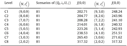
For the SBR-LFC strategy, we examine eight different combina-tions ofNandcf

ias shown inTable 3. From level C1 to C8, the num-ber of suppliers is decreasing from 9 to 2, while the suppliers’ ﬁxed ordering costcf

i is decreasing from 0.9 to 0.2. At each level, total 81 different scenarios are created to evaluate the performance of the given strategy, in which Qitakes three levels at (4, 5, 6),kitakes three levels at (0.08, 0.10, 0.12), U takes three levels at (1.0, 1.2, 1.4), andntakes three levels at (0.7, 0.8, 0.9). The forth col-umn inTable 3gives the average costs over 81 scenarios at state (0, 0).Table 3shows that the average total cost appears monotonic increasing as the level of SBR-LFC increases, and the best trade-off point is at N;cf

i

[image:9.595.71.267.89.208.2]

¼ ð9;0:9Þwith the total expected cost 202.71. Fig. 1.Impact of supplier capabilities on the system performance. (Diamond line –

[image:9.595.310.563.114.206.2]

Case 1; square line – Case 2; triangle line – Case 3; cross line – Case 4).

Table 1

Performance of SBR-HDC strategy.

Level (N,Qi) _{Scenarios of} _k_i;U;_n_;_cf i

_J_{(0, 0)}

A1 (9, 1) 81 259.48

A2 (8, 2) 81 211.88

A3 (7, 3) 81 207.97

A4 (6, 4) 81 212.83

A5 (5, 5) 81 222.63

A6 (4, 6) 81 238.09

A7 (3, 7) 81 262.81

A8 (2, 8) 81 306.04

Table 2

Performance of SBR-SRD strategy.

Level (N,ki) _{Scenarios of} _Qi;U;_n_;cf i

J(0, 0)

B1 (9, 0.03) 81 391.60

B2 (8, 0.05) 81 292.43

B3 (7, 0.07) 81 246.05

B4 (6, 0.09) 81 221.34

B5 (5, 0.11) 81 208.24

B6 (4, 0.13) 81 203.53

B7 (3, 0.15) 81 207.99

B8 (2, 0.17) 81 229.17

Table 3

Performance of SBR-LFC strategy.

Level _N;_cf i

Scenarios of (Qi,ki,U,n) J(0, 0) _N;_cf i

J(0, 0)

[image:9.595.309.564.548.640.2] [image:9.595.311.564.684.776.2]

(10)

The reason that we did not see the U-shape of the cost function is the setting of the cases, e.g. the cases have not covered the suffi-ciently large range, or the fixed ordering cost is not decreasing quickly enough to cancel out the effect of the supplier base reduc-tion. For example, if we re-design level C1 to C8 to be those in the fifth column inTable 3, we would have the average costs over 81 scenarios at state (0, 0) in the sixth column. Clearly, we can now see the U-shape of the average cost with the best trade-off at

N; cf i

¼ ð6;1:8Þ.

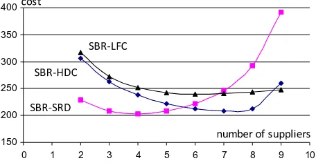
To have a more intuitive view of the performances at different levels of the supplier base reduction strategies, the average costs are shown inFig. 2, in which the data in the last column ofTable 3

are used for SBR-LFC. FromTables 1–3andFig. 2, it veriﬁes the re-sults inConjecture 1, i.e. the total cost is of U-shape under each of three supplier base reduction strategies. It should be pointed out that we have varied two parameters on discrete basis to represent different levels of supplier base reduction strategies, this may not cover all real settings and effects. In addition, in practice there may be extra costs associated with supplier capability improve-ment or maintaining the supplier base, which may impact on the best trade-off point under the supplier base reduction strategies.

7.3. Supplier differentiation

This sub-section aims to illustrate the results about supplier dif-ferentiation inProposition 4, and examine the control structure of the optimal integrated procurement and production policies. The common system parameters are set as follows: b= 0.1; c1= 1.0;cþ

2¼2:0; c2¼8:0; cp= 1.0; U= 1.0; n= 0.8. To simplify the discussion, we consider the cases with two suppliers, i.e. N= 2, but they have different supply capabilities. We vary one parameter at a time to examine four cases below.

Case D1:Supplier 1 has a delivery capacityQ1= 5, and

sup-plier 2 hasQ2= 6; other parameters are the same for both suppliers, i.e.cf

i ¼0:5; cvi ¼0:2; ki¼0:1, fori= 1, 2.

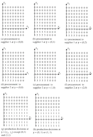
Case D2:Supplier 1 has ordering ﬁxed costcf1¼0.5, and

sup-plier 2 hascf

2¼1.0; other parameters are the same for both suppliers, i.e.Qi¼5; cvi ¼0:2; ki¼0:1, fori= 1, 2.

Case D3:Supplier 1 has ordering variable costcv1¼0.2, and

supplier 2 hascv

2¼0.4; other parameters are the same for both suppliers, i.e.Qi¼5; cfi ¼0:5; ki¼0:1, fori= 1, 2.

Case D4:Supplier 1 has delivery ratek1= 0.1, and supplier 2

hask2= 0.2; other parameters are the same for both suppli-ers, i.e.Qi¼5; cfi ¼0:5; cvi ¼0:2, fori= 1,2.

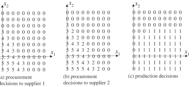
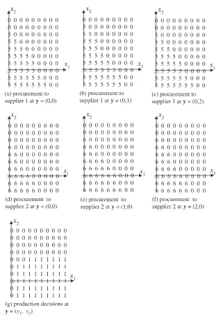
The optimal procurement and production decisions in the above four cases are partially shown in the (x1,x2) plane in Figs. 3–6, respectively, in which the numbers indicate the optimal order sizes (for the procurement decisions) or whether the manufacturer

should produce products (1 represents producing with rate U, and 0 represents producing nothing), and their positions corre-spond to the system state x= (x1,x2). For example, at the state

x= (3, 0) inFig. 3, the optimal procurement decisions to both sup-pliers are the same with an order size 5, whereas the optimal pro-duction decision is producing with the rate U. The results in

Figs. 3–6illustrate the qualitative results inProposition 4. Namely,

the order sizes to the suppliers with higher supply capability are not less than that to the supplies with lower supply capability.

Fig. 4conﬁrms the results in Proposition 4(ii), i.e. non-zero

pro-curement decisions to the suppliers with higher fixed ordering cost are indeed the same as that to the suppliers with lower fixed order-ing cost. More importantly, through numerical examples we are able to quantify the differences between the procurement deci-sions to different suppliers given the different supplier capabilities. In addition, the results inFigs. 3–6also illustrate the structural characteristics of the optimal procurement and production deci-sions. For example, the optimal procurement decisions to each supplier are characterised by two switching regions (one with no order and the other with non-zero orders), and the order size shows the monotonic property with respect to the raw material and finished goods inventory levels. The optimal production deci-sions can also be characterised by two switching regions (one with producing nothing and the other with producing the rateU). The boundary curves between two switching regions are monotoni-cally increasing or decreasing. More specifimonotoni-cally, the procurement decisions may be approximated by a set of (s,S)-type policies con-strained by the delivery capacity, e.g. inFig. 3(a) and (b), the opti-mal procurement decisions are determined by the (s,S) policy with s= 5 and S= 8 constrained by the delivery capacity Q1= 5 and Q2= 6 whenx2= 0 (i.e. the order size is given by: max{Sx1,Qi}

forx16_{s; and 0 for}_x1_>_{s); and with}_s_{= 4 and} _S_{= 8 constrained}

by the delivery capacityQ1= 5 andQ2= 6 whenx2= 1. As for the production decisions, it appears to be fairly robust to system parameters (e.g. exactly the same inFigs. 3–5, and slightly different

fromFig. 6). The implication is that based on the characteristics of

the optimal policy, we are able to construct near-to-optimal but much simpler parameterised policies to determine the procure-ment and production decisions (Song, 2013).

7.4. The case with non-adjustable outstanding orders

This sub-section considers the cases with non-adjustable out-standing orders. It consists of three parts. The ﬁrst part examines the impact of supplier capabilities on the system performance, in which the results are compared to the cases with adjustable out-standing orders; the second part examines the supplier differenti-ation and the decision structure of the optimal policies; and the third part presents a full factorial experiment to evaluate the im-pact of various factors and their interactions on the system perfor-mance. We limit our experiments within the situations of two suppliers to avoid the high dimension of the state space and the computational difﬁculty.

7.4.1. Impact of supplier capabilities on the system performance The common system parameters are set as follows: b= 0.1; c1= 1.0; cþ2¼2:0; c2¼8:0; cp= 1.0;U= 1.0;n= 0.8. Assume two suppliers have the same supply capabilities. We vary one parame-ter at a time to examine three cases: (i) the suppliers’ delivery capacity (Qi) varies from 3 to 4, 5, 6, 7, 8, and 9; while

N¼5; ki¼0:1; cf

i ¼0:5. (ii) the suppliers’ delivery rate (ki) varies from 0.04 to 0.06, 0.08, 0.10, 0.12, 0.14, and 0.16; while N¼5; Qi¼5; cfi ¼0:5. (iii) the ﬁxed ordering cost (c

f

iÞvaries from 0.3 to 0.4, 0.5, 0.6, 0.7, 0.8, and 0.9; whileN= 5,Qi= 5,ki= 0.1. The results of three cases are given inTables 4–6respectively, in which the second column is the optimal cost under the adjustable

150 200 250 300 350 400

0 1 2 3 4 5 6 7 8 9 10

[image:10.595.44.272.93.211.2]

(11)

[image:11.595.152.457.91.228.2] [image:11.595.148.457.266.403.2]

Fig. 3.The optimal procurement and production decisions in case D1.

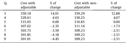
[image:11.595.152.451.437.576.2] [image:11.595.152.460.610.750.2]

(12)

outstanding order assumption, the forth column is the optimal cost under the non-adjustable outstanding order assumption, the third and ﬁfth columns are the percentage of cost changes from the ref-erence case (the row corresponding to 0.00%) under two assump-tions respectively.

FromTables 4–6, it can be seen that the monotonic properties of

the cost function with respect to the key system parameters such as supplier delivery capacity, delivery rate, and ﬁxed ordering cost are preserved for the cases with non-adjustable outstanding or-ders. More interestingly, the percentages of the cost changes after varying the system parameters compared to that of the reference point are very close in two cases (under adjustable and non-adjust-able assumptions). Comparing the optimal costs under two assumptions, it shows that the cost under the adjustable outstand-ing order assumption is slightly lower than that under the non-adjustable outstanding order assumption. This is in agreement with the intuition since the adjustable outstanding order assump-tion provides more ﬂexible opassump-tions for the manufacturer to man-age the raw material procurement.

7.4.2. Supplier differentiation

Consider the same cases with two suppliers having different supply capabilities in Section7.3. Note that the procurement and production decisions are now depending on not only the inventory levels of raw materials and ﬁnished goods, but also the sizes of the outstanding orders to both suppliers. As examples, the optimal procurement and production decisions for cases D1 and D4 are partially shown in Figs. 7 and 8 respectively. For example,

Fig. 7(a) describes the optimal procurement decisions to supplier

1 in the (x1,x2) plane when there is no outstanding order to both suppliers; Fig. 7(b) and (c) describes the optimal procurement decisions to supplier 1 when there is an outstanding order to sup-plier 2 with the order size being 1 and 2 respectively;Fig. 7(d)–(f) describes the optimal procurement decisions to supplier 2 when the outstanding order to supplier 1 being 0, 1 and 2.Fig. 7(g) de-scribes the optimal production decisions at any state of the out-standing orders. It should be pointed out that when there are non-zero outstanding orders to both suppliers, the procurement decisions to both suppliers are forced to be zero due to the assumption that only one outstanding order is allowed to each supplier at any time and they are not adjustable once issued.

The results inFigs. 7 and 8reveal that the qualitative results in

Proposition 4 are generally preserved for the cases with

non-adjustable outstanding orders. Namely, the order sizes to the sup-pliers with higher supply capability are not less than that to the supplies with lower supply capability. However, it is noted that in the case D1 when the echelon inventory level (i.e.x1+x2) or the raw material inventory level exceeds a certain level, the opti-mal policy may place an order to supplier 1 (with lower delivery capacity) but place no order to supplier 2 (with higher delivery capacity). This may be interpreted as follows. When there are ade-quate echelon inventories or raw material inventories in the sys-tem, it is reasonable to place a relatively smaller order to the lower capacity supplier and reserve the opportunity and ﬂexibility of placing a larger order to the higher capacity supplier to buffer against future uncertainty.

In addition, a few interesting points can be observed fromFigs. 7

and 8. Firstly, the structural properties of the optimal procurement

and production policies such as switching control regions and monotonicity of the boundary curves are very similar to the case with adjustable outstanding orders; however, the non-zero order size appears to be a constant that is equal or close to the maximum delivery capacity inFigs. 7 and 8. This implies that it is more appro-priate to approximate the optimal procurement policy using a ser-ies of (r,Q) policser-ies rather than the (s,S) policser-ies. For example, in

Fig. 7(a), the optimal procurement decisions can be determined

by the (r,Q) policy withr= 4 andQ= 5 whenx2= 0 or 1 (i.e. a ﬁxed order sizeQ is placed whenx16_{r); and in}_{Fig. 7}_{(d), the optimal}

procurement decisions can be determined by the (r,Q) policy with r= 3 andQ= 6 whenx2= 0, and withr= 2 andQ= 6 whenx2= 1. Secondly, comparing the procurement decisions at y=(0, 0) with that aty= (0, 1) or (1, 0), the order sizes aty= (0, 0) are generally not greater than that aty= (1, 0) or (0, 1). This can be explained by the fact that at the statey= (0, 0), the manufacturer can place two new orders simultaneously whereas at the statey= (1, 0) or (0, 1) it can only place one new order. The order sizes aty= (0, 1) are not smaller than that aty= (0, 2), which is intuitively true con-sidering the size of the existing outstanding order. Thirdly, the pro-duction decisions are rather insensitive to the system parameters and to the statuses of the outstanding orders. This observation is useful when designing sub-optimal and easy-to-implement pro-duction policies.

7.4.3. Impact of various factors and their interactions on the system performance

This section employs a full factorial experiment design to inves-tigate the impact of various factors and their interactions on the system performance. This technique allows the effects of a factor to be estimated at several levels of the other factors, which can yield conclusions that are valid over a wide range of parameter set-tings (Montgomery, 1991). We assume two suppliers have the same supply capability and focus on the ﬁve main factors

Qi;ki;U;n;cfi

[image:12.595.300.554.110.197.2]

. Each factor takes three levels, e.g. the suppliers’ delivery capacityQifrom (5, 6, 7), the raw material delivery rate Table 5

Impact of suppliers’ delivery rate on the system cost.

ki Cost with adjustable % of change Cost with non-adjustable % of change

0.04 474.29 50.55 474.42 49.73

0.06 406.67 29.09 407.12 28.49

0.08 354.43 12.51 355.48 12.19

0.1 315.03 0.00 316.85 0.00

0.12 285.26 9.45 287.97 9.11

0.14 262.43 16.70 265.98 16.05

[image:12.595.33.286.111.198.2]

0.16 244.55 22.37 248.85 21.46

Table 4

Impact of suppliers’ delivery capacity on the system cost.

Qi Cost with adjustable

% of change

Cost with non-adjustable

% of change

3 359.18 14.01 359.29 12.88

4 329.61 4.63 330.25 4.07

5 315.03 0.00 316.85 0.00

6 307.62 2.35 311.16 1.73

7 303.73 3.59 309.23 2.31

8 301.85 4.18 309.23 2.31

9 301.01 4.45 309.23 2.31

Table 6

Impact of ﬁxed ordering cost on the system cost.

cf

i Cost with adjustable

% of change

Cost with non-adjustable

% of change

0.3 311.66 1.07 313.61 1.02

0.4 313.36 0.53 315.23 0.51

0.5 315.03 0.00 316.85 0.00

0.6 316.68 0.52 318.47 0.51

0.7 318.32 1.04 320.09 1.02

0.8 319.95 1.56 321.70 1.53

[image:12.595.33.279.240.328.2]

(13)

kifrom (0.10, 0.12, 0.14), the maximum production rate U from (1.0, 1.2, 1.4), the demand arrival ratenfrom (0.60, 0.72, 0.84), and the ﬁxed ordering cost coefﬁcientcf

i from (0.5, 0.6, 0.7). Other sys-tem parameters are set the same as those in Section7.1. The above ranges of the ﬁve factors are generated by increasing the value of each factor by 20% from its lowest level, which ensures that the systems have reasonable utilisations and stable in long term (i.e. maximum supply capacity exceeds the demand rate). Note that

ki,U, andnrepresent the degree of three different types of

uncer-tainties, the full factorial analysis can shed light on their relative importance and interactive impact on the system performance.

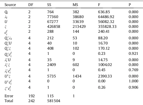
In total there are 35_{= 243 different scenarios in the full factorial} experiment. We perform the analysis of variance (ANOVA) to investigate the effects of these factors and their interactions on the total cost. For each factor, the degrees of freedom (DF), sums of squares (SS), mean square (MS),Fvalue (F) and probability (P) are given inTable 7.

For a given conﬁdence interval 0.05, which is deﬁned as the acceptance probability that an important factor is incorrectly rejected, all factors or interactions with a value of P< 0.05 are

statistically significant. It can be seen fromTable 7that all factors have valuesP< 0.05 and are therefore statistically significant with-in the ranges considered. From theFvalue inTable 7, it shows that the forth factor (demand arrival rate) has the largest effect on the cost; the second factor (suppliers’ delivery rate) and the third (manufacturer’s production rate) have the second largest effect on the cost. This indicates that three factors representing three types of uncertainties have much more significant impact on the cost than the other two factors (i.e. the suppliers’ delivery capacity and the suppliers’ fixed ordering cost). The interactions with the factorcf

i (i.e. the fixed ordering cost) are statistically insignificant within the ranges under consideration, whereas all other interac-tions have significant effect since theirPvalues are less than 0.05.

8. Conclusions

[image:13.595.143.464.81.541.2]

(14)

presence of multiple types of uncertainties such as uncertain mate-rial supplies, stochastic production times, and random customer demands. We focus on the supplier management issues such as supplier base reduction and supplier differentiation. Our main con-tributions include: (i) a mathematical model and a solution meth-od are presented for the optimal procurement and prmeth-oduction problem with multiple suppliers and multiple uncertainties; (ii) Under the assumption that the supply chain is integrated in the sense that the suppliers and the manufacturer have an agreement that the manufacturer can adjust the order quantity at any future decision point before it arrives, we are able to analytically establish the qualitative relationships between the supplier base size and the system performance, and between the suppliers’ capabilities (such as delivery capacity, delivery lead-time and reliability, and ordering cost) and the system performance. We also establish the qualitative relationship between the procurement decisions to dif-ferent suppliers so that we can difdif-ferentiate suppliers. The model further enables us to quantify the above relationships and achieve the best trade-off between the supplier base reduction and the

[image:14.595.137.449.85.545.2]