Distributed Stochastic Cross-layer Optimization for
Multi-hop Wireless Networks with Cooperative
Communications
Shusen Yang, Zhengguo Sheng, Julie A. McCann, and Kin K. Leung
Imperial College London
Abstract—Cooperative communication has been shown to have great potential in improving wireless link quality. Incorporating cooperative communications in multi-hop wireless networks has been attracting a growing interest. However, most current re-search focuses on either centralized solutions or schemes limited to specific network problems. In this paper, we propose a distributed framework that uses Network Utility Maximization (NUM) to optimize the following joint objectives: flow control, routing, scheduling, and relay assignment; for multi-hop wireless cooperative networks with general flow and cooperative relay patterns. We define two special graphs, Hyper Forwarding Graphs (HFG) and Hyper Conflict Graphs (HCG), to represent all possible cooperative routing policies and interference rela-tions among the cooperative relays respectively. Based on HFG and HCG, a stochastic mixed-integer non-linear programming problem is formulated. We then propose lightweight algorithms to solve these in a fully distributed manner, and derive the theoretical performance bounds of these proposed algorithms. Simulation results verify our theoretical analysis and reveal the significant performance gains of our framework, in terms of throughput, flexibility, and scalability. To our knowledge, this is the first distributed cross-layer optimization framework for multi-hop wireless cooperative networks with general flow and cooperative relay patterns.
I. INTRODUCTION
Cooperative communication schemes [1]–[7] are well-recognized as an effective way of exploiting spatial diversity to significantly improve the quality (e.g. capacity and reliability) of wireless links at the physical layer. The key idea is that mul-tiple wireless single-antenna devices cooperatively share their antenna resources and aid each other’s wireless transmission by forming virtual and distributed antenna arrays. During the last decade, such schemes have been extensively studied at the physical layer in two-hop wireless networks.
Recently, there has been an increasing interest in incor-porating cooperative communication schemes in multi-hop wireless networks [8]–[12] to improve the end-to-end network performance such as throughput [9], energy consumption [13], and reliability [12]. However, these proposed schemes are often centralized or restrictive. Specifically, most of them focus on specific cases such as network topologies (e.g. two-hop networks [9]), traffic flow patterns (e.g. single source-destination pairs [8]), network problems (e.g. routing [13]), or cooperative relaying patterns (e.g. single relay [10]).
For cross-layer optimization in multi-hop networks with general network topologies and traffic flow patterns, Net-work Utility Maximization (NUM) approaches [14]–[16] have
shown to be powerful tools, but most of them focus on wireless networks with pure SISO links. The use of NUM techniques for wireless cooperative networks is however very few [9], [17]. Further, such work is still restricted to specific network topologies (e.g. two-hop networks [9]) or cooperative relay patterns (single relay [17]).
In this paper, we propose a distributed cross-layer optimiza-tion framework for joint flow control, routing, scheduling, and relay assignment in multi-hop wireless cooperative networks with general network topologies, cooperative relaying, and traffic flow patterns, by combining the NUM technique with novel graph-theoretic approaches. Our overarching goal is to design lightweight and efficient distributed algorithms for maximizing network utility (e.g. throughput and fairness) by exploiting the broadcast advantages of wireless transmissions, the potential capacity gains of cooperative transmissions, and useful interactions among different layers.
The proposed framework considers time-varying Rayleigh-fading channels, and the following three one-hop wireless transmission schemes [13]: direct transmission over input output (SISO) links, broadcast over virtual single-input multiple-output (SIMO) links, and cooperative beam-forming (e.g. [18]) over virtual multiple-input single-output (MISO) links. We assume that time division multiple access (TDMA) is adopted at the link layer and use the commonly-used node exclusive model (e.g. [19], [20]) to model interfer-ence among hybrid direct, broadcast, and beamforming links. The following four key issues are addressed in our framework. • Cooperative Scheduling and Relaying. At the link layer, how to schedule the hybrid direct, broadcast and beamforming links for concurrent contention-free trans-missions. This scheduling problem also determines co-operative relay assignment: the scheduling of a virtual SIMO or MISO link implies that a set of nodes incident to the scheduled link are assigned as cooperative relays. • Cooperative Routing. At the network layer, how to compute optimal end-to-end cooperative routing policies (single path or multipath), which consist of sequences of hybrid one-hop direct, broadcast, and beamforming links. • Flow Control.At the transport layer, how to allocate the rate of each flow to achieve network utility optimization and system stability (i.e. the allocated flow rates can be afforded by the underling routing, scheduling and time-varying channel capacities).
problem [13], [21] and the optimal scheduling problem (even for wireless networks with pure direct links) [22] have been proven to be NP-hard in general. Consequently, the tradeoff between complexity and optimality is also a key issue considered in our framework.
A. Our Contributions
The major contributions of this paper are summarized as follows:
• We propose two specific concepts of graphs, the Hy-per Forwarding Graph (HFG) and the HyHy-per Conflict Graph (HCG), to respectively represent general end-to-end cooperative routing policies and interference relations among hybrid direct, broadcast, and beamforming links under the node-exclusive interference model. Based on HFG and HCG, we formulate a stochastic mixed-integer non-linear programming problem for joint flow control, routing, scheduling, and cooperative relay assignment in multi-hop wireless cooperative networks, characterized by the Rayleigh-fading channel model.
• A distributed global optimal algorithm is developed to solve the formulated optimization problem by using La-grangian duality theory and novel graph-theoretic ap-proaches. The proposed algorithms automatically adjust flow rates, as well as select forwarding links and coop-erative relays based on the time-varying channel state. • As the optimal solution to the cooperative scheduling
problem has high computational complexity, we propose a lightweight greedy algorithm to solve the cooperative scheduling problem in a fully distributed way. In addition, the number of all possible cooperative relays could be of the exponential order of the total number of nodes in the network, but most of them are not useful for forwarding data. To further reduce the system complexity, we develop an effective scheme to delete such useless relays. • We provide formal proofs for the optimality and
con-vergence of the global distributed system, and derive the worst-case performance and overhead bounds of the greedy scheduling algorithm. Simulation results demon-strate that 80.2% network throughput improvement can be achieved by incorporating cooperative communications, and the performance of the distributed greedy scheme with much less convergence time is close to the optimal (more than 88%).
• We also provide three useful extensions: global outage probability minimization, all possible cooperative routing policies, and Lyapunov queueing systems, which demon-strate the flexibility of our framework.
B. Related Work
1) Multi-hop Wireless Cooperative Networks: Recently, there have been increasing research efforts in applying cooper-ative communication in multi-hop wireless networks [8]–[12], [23], [24]. For distributed approaches, the cross-layer schemes proposed in [23], [25] are heuristic and cannot provide perfor-mance guarantees. Based on dynamic programming, energy-aware cooperative routing algorithms are developed in [13],
[26] for general cooperative relaying patterns and network topologies, as for our paper. However, their approaches con-sider the delivery of individual messages rather than end-to-end flows. [12] presents a distributed routing scheme to minimize end-to-end outage probability based on the Bellman-Ford algorithm. However, it is limited to the linear network topologies and single source-destination pair. [8] presents a centralized approach to maximize the rate of a single end-to-end flow. [10] aims to maximize the minimal rate of multiple competing flows (i.e. max-min optimization). However, this work is not only centralized and deterministic, but also only considers the specific three-node model for cooperative relay-ing.
2) Network Utility Maximization: NUM techniques [14], [27], [28] such as Lagrange duality and Lyapunov optimization have been studied extensively for various problems in wireless networks with pure direct links, including routing [29], flow control [30], random access control [28], power control [31], and scheduling [32]. In addition, NUM-based approaches have also been used in network coding and opportunistic routing to exploit broadcasting advantages (i.e. receiver-side diversity) of wireless communications [33]–[35], which are similar to our work. However, none of above focus on wireless networks with cooperative communications that exploit the wireless diversities on both the receiver and transmitter sides. Recent comprehensive surveys of NUM research can be found in [14]–[16].
3) Using NUM in Wireless Cooperative Networks: Little NUM-based research exists for wireless cooperative networks [9], [17]. In [9], a centralized approach is proposed that extends backpressure algorithms totwo-hopwireless networks with general cooperative communication patterns. In contrast to [9], we focus on a fully distributed approach for multi-hop wireless cooperative networks with arbitrary network topologies. [17] formalizes a deterministic convex optimiza-tion problem for joint congesoptimiza-tion control and power control. However, it assumes restrictive cooperative relaying (i.e. single relay) and traffic patterns (single commodity). More impor-tantly, wireless interference is not addressed. By taking general cooperative relaying patterns, time-varying channel states, and interference among hybrid direct, broadcast, and beamforming into account, the stochastic optimization problem, considered in our framework, is much more realistic and challenging than that in [17].
Compared with the above related work, our cross-layer framework considers not only the distributed and stochastic nature of multi-hop wireless networks, but also general net-work topologies, traffic flow patterns, and cooperative relaying patterns. To our knowledge, this is the first work that takes all these issues into account for multi-hop wireless cooperative networks.
C. Outline
simulations. Finally, we conclude the paper in Section 6. All proofs are placed in Appendices A–D, which can be found in the supplemental material.
II. SYSTEMMODEL
A. Channel Model
We consider a set of statically-deployed nodes that inter-communicate through wireless links. The system operates at discrete time slotst={0,1, ...}. Each node is equipped with a single omnidirectional antenna. For a wireless transmission, the signal-to-noise ratio (SNR) at the destinationyfrom source xcan be modeled as
SN Rx,y =PxHx,y/BN0 (1)
wherePxis the transmission power of x,B is the channel bandwidth, N0 is the noise spectral density, and Hx,y is the power gain. We assume that the transmission power is fixed but not necessarily identical for different nodes. Considering both path loss and Rayleigh fading, Hx,y is exponentially distributed with mean Hx,y = dis−x,yα, where disx,y is the Euclidean distance between nodes x and y, and α is the path loss exponent.Hx,y is assumed to be independently and identically distributed (i.i.d.) over the time slot. We further assume that power gain is independent across the links.
The wireless network can be described as a directed graph G(N, L), whereN is the set of all nodes andLis the set of all direct transmission links (i.e. SISO links). A link (x, y)∈L is considered to exist if the long-term meanSN Rx,y is larger than a predefined small threshold; all other weak links are ignored. Every link (x, y)∈Lcan communicate using direct transmissions. The link capacity of(x, y)is
cx,y =Blog2(1 +SN Rx,y) (2)
It is worth noting that the actual transmission data rate should be smaller than the link capacity. To focus on the systematic cross-layer approach, we do not consider specific physical-layer details (e.g. modulation and coding), and we assume that (2) is the maximum transmission data rate that can be achieved without a decoding error1. However, the essence of our cross-layer approach is nonetheless preserved.
LetNx={y|(x, y)∈L}be the set of all one-hop neighbors of a node x. Besides direct transmission, our model also considers the following two kinds of one-hop transmission schemes:
Broadcast. A nodex can broadcast a message to a set of nodesRS⊆Nx, |RS| ≥2. In order to ensure that all nodes in RS can correctly receive the message, the link quality of a broadcast transmission is constrained by the minimum SN Rx,z, z∈RS. Therefore, the capacity of the virtual SIMO link (x, RS)can be defined as:
cx,RS = Blog2(1 + min
z∈RSSN Rx,z) (3) Cooperative Beamforming. If a set of nodes RS ⊆ Ny,|RS| ≥2, have duplicate copies of a message to be for-warded toy, they can phase-align and scale their transmission
1We can also define theϵ−outage capacity such as in [36] to model the
capacity-outage tradeoff.
signals so that the message can be received coherently by y. The destination node receives multiple copies of the same information transmitted through different wireless channels and the equivalent capacity for virtual MISO link (RS, y) is derived as:
cRS,y=Blog2(1 + ∑
z∈RS
SN Rz,y) (4)
For further details and real-world implementation of this physical layer scheme, we refer the reader to [6], [7], [18] and references therein. We assume that the channel capacities (2)-(4) can be estimated at the beginning of every slot. Since power gain Hx,y is i.i.d. over time, the capacities (2)-(4) of direct, broadcast, and beamforming links are also i.i.d. over time.
B. Topology Model and Hyper Forwarding Graph
We denote a relay setas a set of nodes receiving the same broadcasting messages or sending messages through beam-forming. To represent end-to-end cooperative routing policies and all possible relay sets, we define a Hyper Forwarding Graph (HFG) as follows.
Definition 1. A given wireless network G(N, L) has a cor-responding Hyper Forwarding Graph Gf(N∪ R, L∪L(R), whereRis the set of relay sets andL(R)is the set of virtual SIMO and MISO links:
R={RS|x, y∈N, RS ⊆Nx∩Ny, |RS| ≥2)}
L(R) = ∪ x∈N,RS⊆Nx∩R
((x, RS)∪(RS, x))
Figure 1(a) shows an example ofG(N, L). Since node pairs (1, 5) and (2, 4) shares three neighbors{2, 3, 4}and{1, 3, 5} respectively, the corresponding HFG shown in Figure 1(b) has 8 relay sets, as well as 16 virtual SIMO and 16 MISO links, where SISO links are represented as black solid lines and virtual SIMO/MISO links are represented as red dashed lines. Note that although Figure 1 (a) and (b) are illustrated as undirected graph for readability, all the links are bidirectional. HFG can represent a very large class of end-to-end cooper-ative routing polices. In Figure 1, for instance, routing policy 1 → {2, 3} → 5 means that node 1 first broadcasts data to nodes 2 and 3, then they send data to node 5 by beamforming. The generalized version of our framework, which considers all possible cooperative routing polices is provided in Subsection 4.2.
(a) original graph
1 2
3
4 5
a e
b f
g c
h d
(b) HFG
(4,d)
(5,h) (1,2) (2,5) (4,5)
(1,4) (1,3)
(5,3) (4,3) (2,d)
(1,h) (2,3)
(2,a) (4,a)
(2,b) (4,b)
(2,c) (4,c)
(1,e)
(1,f) (5,f)
(5,e) (5,g)
(1,g)
[image:4.612.52.302.52.148.2](c) the complement of HCG Fig. 1. An example of HFG and HCG. The 8 relay sets are: a={1, 3}, b={1, 5}, c={5, 3}, d={1, 3, 5}, e={2, 3}, f={2, 4}, g={3, 4}, h={2, 3, 4}.
C. Hyper Conflict Graph and Link Rate Region
We assume that time division multiple access (TDMA) is adopted at the link layer. We use the commonly-used node exclusive model (e.g. [19], [20]) to model interference, under which no node can transmit or receive simultaneously (in the same slot). This captures the half-duplex nature of the majority of current wireless transceiver hardware. To reflect contention relations among hybrid SISO, virtual SIMO, and virtual MISO links, we define the hyper conflict graph (HCG) as follows: Definition 2: A given HFG has a corresponding HCG
Gc(V, E), where every vertex in V represents a hyper link in the HFG (hence V =L∪L(R)). An edge inE means that the two corresponding transmission links in the corresponding HFG can not be both active at the same time. If two hyper links(i, j),(i′, j′)∈L∩L(R)are in the following three cases, then the edge((i, j),(i′, j′))∈E.
Case 1.Both of them are SISO links: the two sets of nodes
{i, j}and {i′, j′}satisfy {i, j} ∩ {i′, j′} ̸=∅.
Case 2. One hyper link is a virtual SIMO or MISO link and the other is a SISO link: assume i is the relay set, then(i∪ {j})∩ {i′, j′} ̸=∅.
Case 3. Both of them are virtual SIMO or MISO links: assume i and i′ are the two relay sets, then (i∪ {j})∩ (i′∪ {j′})̸=∅.
For instance, Figure 1 (c) shows the complement of the HCG with regards to the HFG in Figure 1 (b). From HFG and HCG, we can clearly see that both the routing topology and interference relation for multi-hop wireless cooperative networks are much more complex than that of traditional wireless networks with pure SISO links.
A given set of hyper links in a HFG can transmit simulta-neously only if it is an independent set2 of the corresponding HCG. Define channel capacity vector c∈ R|+L∪L(R)|, where
each entryclis the random capacity of a hyper linkl defined by (2)-(4). For a givenc, we define the|L∪L(R)|-dimensional contention-free rate vector sk(c) for HCG’s kth independent setIk, where the l’s entry insk(c)is
skl(c) =
{
cl, if l∈Ik 0, otherwise
Then the link rate region for a given network state c is
2An independent set is a set of vertices in a graph, no two of which are
adjacent.
defined as a convex hull of all possible sk(c):
Π(c) ={s(c)|s(c) =∑ k
aksk(c), ak≥0,∑ k
ak = 1}
Hence, for a given c, no |L∪L(R)|–dimensional vector outsideΠ(c)is feasible for any scheduling policy.
D. Multi-commodity Traffic Flow Model
Let D be the set of all commodities (destinations)3 and S⊆N be the set of all source nodes. Let rd
s(t), s̸=dbe the data generation rate of source node sfor commodity d∈D at slott. Define the source rate vectorr(t)∈R|+S|×|D|, where each entry isrsd(t).
Let fi,jd (t) be the data forwarding rate over hyper link (i, j) ∈ L ∪L(R) for commodity d at slot t. We define fi,j(t) =∑d∈Dfi,jd (t). Due to the link capacity constraint, fi,j(t)≤ci,j(t). We define the |L∪L(R)|–dimensional for-warding rate vectorf(t), where each entry isfi,j(t). According to the link rate region constraint,f(t)∈Π(c(t)). Finally, we define the mean rate vectors r = limt→∞1/t
∑
tr(t) and
f= limt→∞1/t
∑
tf(t).
E. Problem Formalization
Based on the HFG structure and the link rate region constraint, the joint flow control, cooperative routing and scheduling problem is formalized as follows ∀i∈N∪ R:
max r,f
∑
s∈S,d∈D Ud
s(rsd(t)) (5)
subject to rd i +
∑
j∈Ni fd
j,i≤
∑
j∈Ni fd
i,j, i̸=d (6)
f(t)∈Π(c(t)),∀t≥0 (7)
where the transport-layer utility function Ud
s(rds(t)) of source node s is a differentiable, increasing, and strictly concave function such as the logarithmic function for the proportional fairness [37]. The objective (5) is to maximize the long-term average of the aggregate utilities, which results in a high throughput and fair flow rate allocation.
Constraint (6) states the flow conservation law at the net-work layer, i.e. for commodity d in a hyper node i, the sum of long-term average forwarding rates allocated to alli’s outgoing links must be not less than that of its all incoming links plus its source rate (note that rid = 0, ∀i /∈ S). In addition, this constraint also implies that flow splitting and multipath routing may be used to achieve the optimality. Since neither specific relay sets nor end-to-end routes are assigned in advance,fd
i,j,(i, j)∈L∪L(R), d∈Drepresents the long-term optimal average cooperative relay set assignments and routing policies.
Constraint (7) considers both physical-layer capacity and link-layer interference constraints, which ensures that f(t) should be in the link rate region for every slot t. Due to the stochastic and discrete nature of Π(c(t)), problem (5) is in
3For notational brevity, we assume that each commodity only has one
∏
Fig. 2. Architecture of the cross-layer framework.
the form of stochastic mixed-integer programming, which is generally difficult to solve (e.g. ♯P-hard [38]).
It worth noting that the form of problem (5) looks similar as existing NUM-based flow control formalizations in wireless networks with pure SISO links e.g. [16], [31]. However, the constraints (6) and (7) are established based on the proposed HFG and HCG respectively rather than the original graph. Therefore, problem (5) has a much more complex structure in terms of cooperative routing and scheduling (e.g. the co-operative routing policies and interference relations in Figure 1)than existing NUM-based flow control problems in wireless networks with pure SISO links.
For notational brevity, this paper defines the objective (5) as the time-average utility ∑s∈S,d∈DUd
s(rds(t)) rather than the utility of time-average source rates
∑
s∈S,d∈DU d
s(rds(t)). Due to Jensen’s inequality,
∑
s∈S,d∈DUsd(rds(t)) ≤
∑
s∈S,d∈DU d
s(rsd(t)). However, the approaches introduced in this paper can be easily extended to maximize the ∑s∈S,d∈DUd
s(rds(t)), by introducing auxiliary variables as in [15].
III. JOINTALGORITHMS FOR FLOW CONTROL, COOPERATIVE ROUTING AND SCHEDULING
This section presents distributed solutions to problem (5). The architecture of the proposed distributed cross-layer frame-work is shown in Figure 2. In the initialization phase, nodes establish the HFG and corresponding data structures based on the originalG(N, L)in a fully distributed manner (Subsection 3.1). For every time slott, each node obtains the Channel State Information (CSI) and computes the capacities of its corre-sponding links according to (2)–(4). Then each node operates a distributed global algorithm (Subsection 3.2) to allocate source rates r(t) and hyper link forwarding rates f(t) based on a congestion price and cooperative scheduling (Subsection 3.3). Here the congestion price is the Lagrangian multiplier associated with constraint (6), and this is proportional to the data queue backlog for a commodity in a node (e.g. [31]). In addition, a complexity reduction scheme is developed in Subsection 3.4 to delete useless cooperative relays and virtual SIMO/MISO links. We assume that all control messages used in our distributed algorithms are error-free.
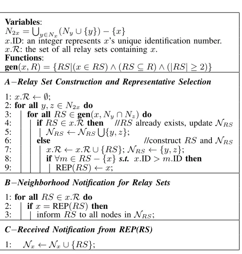
A. Initialization–Distributed HFG Establishment
Variables: N2x=
∪
y∈Nx(Ny∪ {y})− {x}
x.ID: an integer representsx’s unique identification number. x.R: the set of all relay sets containingx.
Functions:
gen(x, R) ={RS|(x∈RS)∧(RS⊆R)∧(|RS| ≥2)}
A−Relay Set Construction and Representative Selection
1:x.R ← ∅;
2:for ally, z∈N2xdo
3: for allRS∈gen(x, Ny∩Nz)do
4: ifRS∈x.Rthen //RS already exists, updateNRS
5: NRS← NRS
∪
{y, z};
6: else //constructRSandNRS
7: x.R ←x.R ∪ {RS};NRS← {y, z};
8: if∀m∈RS− {x}s.t. x.ID> m.IDthen
9: REP(RS)←x;
B−Neighborhood Notification for Relay Sets
1:for allRS∈x.Rdo
2: ifx=REP(RS)then
3: informRSto all nodes inNRS;
C−Received Notification from REP(RS)
[image:5.612.313.562.68.330.2]1: Nx← Nx∪ {RS};
Fig. 3. The pseudocode of Algorithm 1: Distributed HFG establishment for every nodex∈N.
After the deployment of the wireless network G(N, L), every node x ∈ N can obtain its neighbor table Nx. Then, nodexcan establish its two-hop neighbor table which contains the set of nodes N2x =
∪
y∈Nx(Ny ∪ {y}) − {x}, by broadcasting a one-hop beacon that containsNx. To construct HFG in a fully distributed manner, we develop Algorithm 1 shown in Figure 3.
Relay sets are generated by a local functiongen(x, Ny∩Nz) (line 3, part A). For a set of nodes R and a node x ∈ R, gen(x, R)returns the set ofR’s all subsets containingx. For instance, ifRis a set of three nodes{1, 2, 3}, thengen(1,R) returns the set of 3 relay sets:{1, 2},{1, 3}, and{1, 2, 3}. Every nodexstoresx.R, the set of all relay sets containing x. For every relay setRS, the node with the maximal ID in RS is selected as the unique representative of RS, denoted as REP(RS). The set of all other nodes inRS is denoted as REST(RS), i.e. REST(RS) =RS−{REP(RS)}. In addition, hyper neighbor tables Ni are also established for all hyper node i ∈ N ∪ R. Above local topology information estab-lished by Algorithm 1 is acquired to facilitate the distributed solutions for the problem (5). In the later sections, we will see that only REP(RS) is on behalf of RS to participate the distributed operations and all other nodes in REST(RS) may be requested by REP(RS) for some information aboutRS.
B. The Global Distributed Cross-layer Algorithm
L(r,f,λ) = ∑ s∈S, d∈D
(Usd(rds)−λdsrsd)
+ ∑
i∈N∪R
∑
j∈Ni
∑
d∈D
fi,jd (λdi −λdj) (8)
whereλdi is the congestion price for commoditydin hyper node i. Then the corresponding dual problem is
min
λ≽0D(λ) = maxr,f {L(r,f,λ)} (9) where ≽ represents the entry-wise inequality. The dual problem can be hierarchically decomposed into the following two sub-problems:
sub-1: min
λ≽0D1(λ) = maxr≽0 ∑
s∈S, d∈D
(Usd(rsd)−λdsrds)(10)
sub-2: min
λ≽0D2(λ) = maxf∈Π ∑
i∈N∪R
∑
j∈Ni
∑
d∈D
wdi,jfi,jd (11)
where wd
i,j = λdi −λdj and Π is the corresponding static link rate region. The first sub-problem (10) is the flow control problem at the transport layer. For the second sub-problem (11), since(i, j)can be either a SISO, virtual SIMO, or virtual MISO link, the determination of fd
i,j can be interpreted as a hybrid cooperative routing, relay assignment, and scheduling problem, ranging from physical layer to network layer. As can be seen, the global problem decomposes into a number of local optimization problems for every source node (the first sub-problem) and for every hyper link (the second sub-sub-problem), and these sub-problems interact though congestion prices.
Since the objective function of first sub-problem is strictly concave, it admits a unique maximizer as for a givenλds:
(rsd)∗=U d s
′−1
(λds) (12)
where Usd′−1() represents the inverse function of the util-ity function Usd()’s first derivative. For every hyper link (i, j)∈L∪L(R), we define the optimal commodityd∗i,j = arg maxd∈Dwdi,j and corresponding congestion price differ-entialwi,j∗ = maxd∈Dwi,jd . We assignfi,jd =fi,j, ifd=d∗i,j; fd
i,j = 0, otherwise. Then, for a given λ, we have the set of optimal scheduled links F as
F ={fi,j|fi,j∈arg max f∈Π
∑
(i,j)∈L∪L(R)
w∗i,jfi,j} (13)
which is the maximizer of the second sub-problem (11). We will discuss the scheduling problem in detail in Subsection III-C. In this subsection, we suppose that F can be obtained. Due to the convexity and non-differentiability of dual prob-lem (9), it can be solved by using the sub-gradient algorithm. The algorithm starts from the 0th step with initialized λ(0).
At the kth step, the vector g(λ(k))∈R|N∪R|×|D| is defined as a subgradient of dual functionD(λ)at point λ(k), where each entry is
gid(λdi(k)) = ∑ j∈Ni
fi,jd (k)− ∑ j∈Ni
fj,id −rid(k), i̸=d (14)
Therefore, the the congestion price is updated as
λid(k+ 1) =|λdi(k)−γgid(λdi(k))|+, i̸=d (15)
whereγ >0is a constant step size, and|a|+=a, ifa >0;
|a|+= 0, otherwise. If i=d, thenλdi(k) = 0 for allk≥0. Based on by the above deterministic reference system, we develop Algorithm 2 shown in Figure 4; the global cross-layer algorithm for the original stochastic problem (5), in which channel capacity ci,j(t) varies over slot t due to fading. In Algorithm 2, all variables in slottcorrespond to the kth step of the subgradient algorithm in the deterministic reference system. We assign an upper bound rmax of the flow rate maximizer (line 1, part A) to ensure the convergence of Algorithm 2 (Theorems 1 and 2 below). rmax can be set to be sufficiently large to remain the optimality of Algorithm 2. F(t)is the output of the cooperative scheduler at slott, which will be discussed in next subsection in detail. It is obvious that Algorithm 2 shows the flow control, scheduling, and routing (i.e. next hop selection and data forwarding) processes for every slott >0. It also implies the relay set assignment: if a virtual SIMO link(x, RS)or MISO link(RS, x)is scheduled, then relay setRS is assigned in a slott.
Input: Constant step sizeγ, andλdi(0),∀i∈N∪ R, d∈D.
Output: Optimal rds(t),f d
x,y(t), and f d z,RS(t), f
d
RS,z(t), ∀t >
0,x∈N, y∈Nx, RS∈ R, z∈ NRS.
A−A node x at time slot t.
01:ifx∈S then //flow control 02: for alld∈D do
03: rxd(t)←min(rmax, Usd ′−1
(λdx(t);
04:F(t)←transmission scheduler(λ(t)); //scheduling 05:for alli∈ Nx, d∈D do //routing for SISO/SIMO links
06: if(fx,i(t)∈F(t))∧(d=d∗i,j)then
07: fd
x,i(t)←wx,id (t)cx,i(t); //forwarding data ford
08: else
09: fd
x,i(t)←0;
10:for alld∈D, d̸=xdo //updateλdx
11: λdx(t+ 1)← |λdx(t)−γgxd(t)|+
B−A relay set RS at time slot t.
//REP(RS) is on behalf ofRSto participate the operations.
1:F(t)←transmission scheduler(λ(t)); //scheduling 2:for allz∈ NRS, d∈Ddo// routing for virtual MISO links
3: if(fRS,z(t)∈F(t))∧(d=d∗i,j)then
4: fd
RS,z(t)←wRS,zd (t)cRS,z(t); //forwarding data ford
5: else
6: fRS,zd (t)←0;
7 :for alld∈Ddo // updateλd
RS
8: λd
[image:6.612.311.562.315.583.2]RS(t+ 1) =|λdRS(t)−γgRSd (t)|+
Fig. 4. The pseudocode of Algorithm 2: a distributed algorithm for joint flow control, cooperative routing and scheduling. The operations of a node
x∈Nand a relay setRS∈ R.
1) Performance Analysis: Suppose F(t) can be obtained in every slot t > 0, then we can show the convergence of Algorithm 2 by Theorems 1 and 2 as follows. The proofs of the two theorems are presented in Appendix A, available in supplemental material.
Theorem 1. The expected average congestion price E[λ(t)]
converges statistically to the optimal congestion priceλ∗ as
t→ ∞andγ→0, whereλ(t) = 1/t∑tλ(t).
Theorem 2. The dual function D(E[λ(t)]) statistically
where D(λ) = 1/t∑tD(λ).
Since the utility functionUd
s(rxd)is strictly concave, strong duality holds. Hence, the duality gap is zero. Therefore, Theorem 2 implies that the primary variablesrd
s(t)andfi,jd (t) converge statistically to the optimal.
C. Scheduling for Hybrid direct, broadcast and beamforming Links
This subsection focuses on the scheduling problem (11). At time slott, define an undirected link(i, j)with weightwi,js = max{wi,j∗ (t)ci,j(t), wj,i∗ (t)cj,i(t)}, for each corresponding pair of directed hyper links(i, j)and(j, i)on HFG. Then, the net-work state can be represented as an undirected weighted hyper scheduling graph (WHSG) Gw(N∪ R, Lu∪Lu(R), W(t)), whereLu∪Lu(R)is the set of all weighted undirected links. The optimal scheduling problem can be formalized as the following integer programming problem,
max ∑
x,y∈N
βx,ywx,ys +
∑
x∈N,RS∈R
βx,RSwsx,RS
(16) subject to
βx,y =βy,x, βx,y∈ {0,1} (17) βx,RS=βRS,x, βx,RS∈ {0,1} (18)
∑
y∈Nx βx,y+
∑
RS∈Nx
βx,RS ≤1 ∀x∈N (19)
∑
x∈NRS
βx,RS+ ∑
x∈Ny,y∈RS
βx,y ≤1 ∀RS∈ R (20)
The objective (16) is to compute the maximum aggregate weights of all scheduled links. Constraints (17) and (18) state that the binary variable βi,j represents the activity of an undirected link (i, j) ∈ Lu ∪Lu(R). Constraints (19) and (20) ensure that the active links must be contention-free from the aspects of nodes and relay sets respectively, under the node-exclusive model. Denote the optimal solution of problem (16), the set of scheduled links with maximum aggregate total weight, as Sopt(Gw).
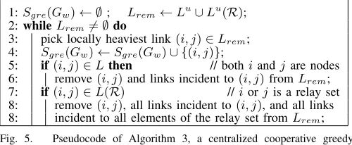
1: Sgre(Gw)← ∅; Lrem←Lu∪Lu(R);
2: whileLrem̸=∅do
3: pick locally heaviest link(i, j)∈Lrem;
4: Sgre(Gw)←Sgre(Gw)∪ {(i, j)};
5: if(i, j)∈Lthen // bothiandjare nodes 6: remove(i, j)and links incident to(i, j)fromLrem;
[image:7.612.53.301.275.416.2]7: if(i, j)∈L(R) //iorjis a relay set 8: remove(i, j), all links incident to(i, j), and all links 8: incident to all elements of the relay set fromLrem;
Fig. 5. Pseudocode of Algorithm 3, a centralized cooperative greedy scheduling scheme.
Since integer programming is NP-hard in general, it is prohibitive to compute the optimal solution of (16) at every slott. To reduce complexity, we propose Algorithm 3 shown in Figure 5, a greedy solution to problem (17), inspired by the Longest-Queue-First (LQF) greedy scheduling schemes used in wireless networks with pure SISO links (e.g. [39]). The output of Algorithm 3 is denoted as Sgre(Gw). To compute
Sgre(Gw)in a fully distributed way, we develop Algorithm 4 summarized in Figures 6 and 7.
Variables:
x.FR: the set of x’s all free relay sets,x.FR ⊆x.R. x.FN: the set ofx’s all free neighbors,x.FN ⊆ Nx.
RS.FN: the set of all free neighbors ofRS∈x.FR.
x.optimal state: one end of thex’s locally heaviest hyper link which could be eitherxitself or a relay setRS∈x.FR. x.optimal neighbor:the other end ofx’s local heaviest link. x.schedule ready: a boolean value represents whetherxis ready to schedule.
x.schedule state: a boolean value that represents whetherxhas been scheduled or not.
Control Messages:
scheduling-apply (SA), scheduling-reply(SR), anddrop Functions:
send(T, source, destination): the source multicasts/unicasts a one-hop control message with type T ∈ {SA, SR, drop} to the destination.
C query(RS): Discussion between REP(RS) and REST(RS) to check whether a link incident toRS is locally optimal of all nodes inRS.
C confirm(RS): when a link incident to relay setRS is sched-uled, REP(RS) informs this information to REST(RS).
Fig. 6. Definitions of Algorithm 4 (distributed greedy scheduling) for a node
x∈N.
In Algorithm 4, a node or a relay set that is not involved in any scheduled hyper link is termed asfree. After initialization in partA, every node x∈N executes and repeats the while loopof partBand processes the triggered events (partsC−E), until the text condition of thewhile loopoccurs, i.e.xitself or a relay set containingxis scheduled (x.scheduled state=true), or xhas no free neighbor (x.FN =∅).
Algorithm 4 has two levels of operations. The upper level is the greedy scheduling for all links inLu∪Lu(R), based on se-lecting the locally optimal link and exchanging three one-hop control messages: schedule apply (SA), schedule reply (SR) anddrop. For a relay setRS, only REP(RS) is on the behalf ofRSfor the upper level scheduling process. The lower level is to ensure that information symmetry between REP(RS) and REST(RS) of a relay setRS∈ R, which is implemented by two functions C query (RS) and cooperative confirm(RS). The interface between the upper and lower level operations is the variablex.scheduled ready. REP(RS) is qualified to send a SA or reply a SR only if REP(RS).scheduled ready=true (line 14 in B and line 10 inC).
At the upper level, every node x selects a local heaviest-weighted free hyper link (i∗x, jx∗) =(x.optimal state,
x.optimal neighbor) from its own point of view. Ifx=i∗x or x =REP(i∗x), then x sends a SA with source i∗x to jx∗ (i.e. x.optimal neighbor) in order to request the scheduling of link (i∗x, jx∗). Ifjx∗is a node,xdirectly sends the SA message to it; otherwisexsends the SA to REP(j∗x) (partB). Either the SA request can be granted (partC), if the link(i∗x, jx∗)is also the locally heaviest link for jx∗; or (i∗x, j∗x) is eventually dropped (partsCandD). If(i∗x, jx∗)∗ is dropped, thenxselects a new locally heaviest link.
[image:7.612.49.299.542.645.2]A−initialization
1: x.FN ← Nx;x.scheduled state←false;x.FR ←x.R;
2: for allRS∈x.FRdo
3: RS.F N← NRS;
B−locally optimal link selection and scheduling apply 01:while(x.scheduled state=false)∧(x.FN ̸=∅)do
02: w∗1←maxj∈x.FNwsx,j; j∗←arg maxj∈x.FNwx,js ;
03: x.optimal state←x;x.optimal neighbor←j∗; 04: x.scheduling ready←false;
05: if∃(RS, y)s.t.RS∈x.FR, y∈RS.F N then
06: w2∗←max(RS∈x.FR,y∈RS.F N)(wRS,ys );
07: (RS∗, y∗)←arg max(RS∈x.FR,y∈NRS)(w
s RS,y);
08: ifw2∗> w1∗then//x.optimal state̸=x
09: x.optimal state←RS∗;x.optimal neighbor←y∗; 10: ifx=REP(x.optimal state)then
11: x.scheduling ready←C query(x.optimal state); 12: else//x.optimal state=x
13: x.scheduling ready←true; 14: ifx.scheduling ready=true then
15: send(SA,x.optimal state,x.optimal neighbor); C−received a(SA, i, j)message
01:ifi=x.optimal neighborthen
02: ifx.optimal state=xthen
03: x.scheduled state←true;
04: send(SR, x, i);send(drop, x, x.FN); 05: for allRS∈x.FR s.t.REP(RS) =xdo
06: send(drop, RS, RS.FN); 07: else//x=REP(x.optimal state) 08: ifx.scheduling ready=false then
09: x.scheduling ready←C query(x.optimal state)); 10: ifx.scheduling ready=true then
11: x.scheduled state←true; 12: send(SR, x.optimal state, i);
13: C confirm(x.optimal state);send(drop, x, x.FN); 14: send(drop,x.optimal state,x.optimal state.FN); 15:else ifx.optimal state=xthen//jis a node,xdeletesi 16: x.FN ←x.FN − {i};
17:else//j is a relay set,xdeletesi
18: x.optimal state.FN←x.optimal state.F N− {i}; D−received a(SR, i, j)message
1: x.scheduled state←true; 2: Ifx.optimal state=x then
3: send(drop, x, x.FN);
4: for allRS∈x.FRs.t.REP(RS) =xdo
5: send(drop, RS, RS.FN); 6: else
7: send(drop, x.optimal state, x.optimal state.F N); 8: C confirm(x.optimal state);
E−received a(drop, i, j)message 1: x.FN ←x.FN − {i}; 2: for allRS∈x.FRdo
3: ifi∈RSthen
4: x.FR ←x.FR − {RS}; 5: ifi∈RS.F Nthen
6: RS.F N←RS.F N− {i};
Fig. 7. Operations of Algorithm 4 (distributed greedy scheduling) for a node
x∈N.
C query (RS) and C confirm (RS) need to communicate between the REP(RS) and the node(s) in REST(RS). We discuss their operations and logical flows based on Figure 8. The action of the C query(RS) function is the two-way handshake between REP(RS) and REST(RS) during [t1,t2]
[image:8.612.320.551.51.208.2]in Figure 8 (a)-(d). If REP(RS) finds that a free link incident to the relay set RS, say l∗, is its locally heaviest link, it sends a Cooperative Apply (CA) message to REST(RS) to check whether l∗ is also locally optimal for all nodes in REST(RS). Every node in REST(RS) responses to REP(RS)
Fig. 8. The time table of distributed scheduling of a hyper link incident toRS, whereNRS∗ denotes the optimal neighbor of REP(RS). (a) and (b) shows successful handshakes between REP(RS) and REST(RS), while (c) and (d) show two unsuccessful cooperative handshakes.
by sending a Cooperative Reply (CR, ack or nack) message carrying the result. If every node in REST(RS) replies an ack, REP(RS).schedule readyis set as true (line 11 in B and line 09 inC), then REP(RS) is qualified to attend the upper level scheduling (i.e. sends a SA or replies a SR); otherwise, REP(RS) deletesRSfrom REP(RS).FR, and selects its new locally heaviest link.
During [t2,t3] shown in Figure 8 (a) and (b), when a link
l∗∈Lu(R)incident to a relay setRS is successfully sched-uled, REP(RS) calls the C confirm (RS) function (line 13 in C and line 8 in D), i.e. REP(RS) multicasts a Cooperative Confirm (CC) message to all nodes in REST(RS) to inform them thatl∗is successfully scheduled (l∗is the locally heaviest link for all nodes in RS). Upon receiving the CC message, every nodey∈REST(RS) setsy.scheduled stateas true, then sends a drop message to all its free neighbors and relay sets RS,y= REP(RS).
It is worth noting that the upper-level control messages SA, SR and drop are sent over one-hop links and the lower-level messages CA, CR and CC may cover two hops (at most two hops), which is feasible because the two-hop neighbor table N2x, x ∈ N was established in the initialization phase (i.e.
Algorithm 1).
1) Performance Analysis: Theorems 3, 4, and 5 below provide analytical results for the communication overhead, convergence and optimality of Algorithm 4 respectively. The proofs of the three theorems and supporting lemmas are presented in Appendix B, available in supplemental material. Theorem 3. The total number of control messages sent by Algorithm 4 is not more than4 + 2 maxRS∈R|RS|per hyper link.
According to Theorem 3, the per hyper link communication overhead of Algorithm 4 is O(1) with respected to|L∪L(R)|, which demonstrates the scalability of Algorithm 4.
Theorem 4.Algorithm 4 terminates for every nodex∈N.
W(Sgre(Gw))≥ 1
maxRS∈R|RS|+ 1
W(Sopt(Gw))
whereW(Sgre(Gw))andW(Sopt(Gw))are the aggregated weights of greedy scheduling Sgre(Gw)and optimal schedul-ing W(Sopt(Gw))respectively.
It is worth noting that Theorem 5 provides a very loose lower bound for the optimality of Algorithm 4. Through simulation in Section 5, we will show that Algorithm 4 can achieve more than 88% performance of the optimal scheduling in practice.
D. Complexity Reduction
It can be seen that |R| and |L(R)| is of the order of |N|2τ, where τ is the average network degree of original graph G(N, L). Therefore, even a small-scale (especially dense) network can produce large-scale HFG and HCG (see the example shown in Figure 1). This results in high system complexity such as the low convergence speed of Algorithm 2. To reduce the complexity, we propose a simple scheme operating in the initialization phase (followed by Algorithm 1), which deletes virtual SIMO and MISO links that would almost never be used to forward data.
Definition 3. Consider two nodes x and y such that |Nx∩ Ny| ≥2, then a long-term 2-Hop Hyper Routing Policy
(2-HHRP) is denoted as a triple (x, i, y),i∈Nx∩Ny. Consider
the flow conservation law and node-exclusive model, the long-term mean capacity of (x, i, y), Cx,i,y, can be approximately
estimated asmin(cx,i, ci,y)/2.
To maximize the aggregate flow rates, Algorithm 2 tends to select hybrid direct and cooperative routes consisting of sequences of 2-HHRP triples (x, i, y), x, y∈N, i∈Nx∩Ny with large capacity and small interference (i.e. small-size i). Hence, we propose a complexity reduction scheme as follows:
A. For all x, y ∈ N,|Nx∩Ny| ≥ 2, delete all broad-cast links (x, RS) and beamforming links (RS, y), if ∃z ∈ RS, s.t. Cx,z,y ≥ Cx,RS,y. This is because that both (x, z, y)and (x, RS, y)have the same routing functionality, but Cx,z,y ≥ Cx,RS,y and (x, z, y) has a smaller interference.
B. For all RS ∈ R, x, y ∈ N, delete broadcast link (x, RS) and beamforming link (RS, y), if RS = Nx∩Ny. The reason is that we can find two hyper nodes i1, i2, i1∩i2 = ∅, i1 ∪i2 = Nx ∩Ny such that the
maximum data rate transmitted by using two 2-HHRP triples (x, i1, y)and(x, i2, y)is larger than using one
2-HHRP triple (x, Nx∩Ny, y). This is formally proved in Theorem 6 below.
Theorem 6.For anyx, y∈N,|Nx∩Ny| ≥2, there exist two
hyper nodes i1, i2, i1∪i2 =Nx∩Ny, i1∩i2 =∅ such that
Cx,Nx∩Ny,y<(Cx,i1,y+Cx,i2,y)/2.
Proof. Please refer to Appendix C, which can be found in supplemental material.
The simulation results (Section 5) show that the proposed scheme can significantly reduce system complexity. However, formal analysis of this scheme remains part of our future work.
IV. EXTENSIONS
A. Outage Probability Minimization
Outage probability [1] is a key metric in cooperative com-munications. Our framework can be extended to balance the tradeoff between network utility and global (multipath end-to-end) outage probability, by introducing an aggregated penalty −V∑(i,j)∈L∪L(R)Pout
i,j in the original objective function (5). Here, Pout
i,j is the outage probability for a hyper link (i, j), which is a complex non-linear function of forwarding rate fi,j. V ∈ [0,+∞] is control parameter that is chosen to affect a desired tradeoff between the network utility and outage probability.
We use a linear approximation for outage probability, Pout
i,j ≈costi,jfi,j, (i, j)∈L∪L(R), where the expression of costi,j is provided in Theorem 7 below.
Theorem 7. For Rayleigh-fading channels, the closed-form expression of costi,j is
costi,j=
ln(2)SN Ri,j/B i, j∈N
|j|(ln(2))|j|∏
y∈jSN Ri,y/B i∈N, j∈ R ln(2)∑x∈iQx/B i∈ R, j∈N
where
Qx=
∏
m∈i(SN Rm,j)
∏
m∈i,m̸=x(SN Rm,j−SN Rx,j)
(21)
Proof. Please refer to Appendix D, which can be found in supplemental material.
A fully distributed cross-layer framework that jointly op-timizes network utility and global outage probability can be obtained by redefine wi,j(t) as λi(t)−λj(t)−V costi,j in (subproblem11). By redefining wi,j(t), all proposed algo-rithms can be directly used without modification.
B. All Possible Cooperative Routing Policies
The currently-defined HFG considers a large class of coop-erative routing policies, but not all possible routing policies. For instance, assume that there is a flow with source node 4 and destination node 2 in Figure 1, the following routing policy can not be presented by currently-defined HFG: node 4 first broadcasts data to{3, 5}, then{3, 5}send data to 1 by using beamforming, and finally{1, 3, 5}send data to 2 using beamforming.
Definition 4. For a given HFG Gf(N ∪ R, L∪L(R), the
completed hyper forwarding graph (C-HFG),Gc
f(R′, L′(R′),
represents all possible end-to-end cooperative routing policies, where
R′ = (∪ x∈N
{x})∪( ∪ RS∈R,y∈NRS
{y} ∪RS)∪R
L′(R′) ={(RS1, RS2)|RS1, RS2∈ R′, RS1̸=RS2,
∃x∈RS1, y∈RS2 s.t. x∈Ny}
as {4} → {3,5} → {1,3,5} → {2}. The well-known three-node cooperative relay pattern [1], [10], [17] can also be represented easily by using C-HFG. In Figure 1, for instance, {1} → {1,2} → {3}represents the routing policy that node 1 first sends data to node 2 via direct transmission, then nodes 1 and 2 send data to node 3 using beamforming. Compared with HFG, C-HFG has more vertexes and edges.
At the physical layer, we define the sets of all possible SISO and virtual SIMO/MISO links Lphy as
Lphy = ∪
x∈N,i⊆Nx∩R′
{({x}, i)} ∪ {(i,{x})}
The capacities of each link(i, j)∈Lphy can be computed by (2)–(4).
At thelink layer, we bridge the gap between network-layer routing policies and actual physical-layer data transmissions by defining a link mapping rule
M : L′(R′)→Lphy
For an edge (RS1, RS2) ∈ L′(R′), if RS2 ⊂ RS1, then
M(RS1, RS2) =∅, sinceRS1 can send data toRS2without
any physical-layer transmission; otherwise,
M(RS1, RS2) =
{(i, j)|i⊆RS1, j⊆RS2−RS1∩RS2 (i, j)∈Lphy}
For instance, in Figure 1, edge ({3,4},{3,5}) can be mapped into two SISO links (4, 5) and (3, 5), and one virtual MISO link ({3,4}, 5).
Now we discuss how to generalize our framework to con-sider all possible cooperative routing policies. We can first establish C-HGF in a distributed way by slightly modifying Algorithm 1. Then we can develop a global algorithm similar as Algorithm 2 by introducing a congestion price λdRS for every relay set RS ∈ R′ and commodity d ∈ D. For (RS1, RS2)∈ L′(R′)in slot t, an unique optimal
physical-layer transmission link
(i∗, j∗) = arg max
(i,j)∈M(RS1,RS2),
ci,j(t)
can be obtained. Since (i∗, j∗) ∈ Lphy, Algorithm 4 can be directly used for scheduling without modification.
C. Stochastic Queueing Networks
Lyapunov queuing (e.g. [31]) is a popular research area in stochastic network optimization and shows great promise for practical implementations. Our current dual-decomposition based framework can be transferred to the Lyapunov backpres-sure system, with the following three simple modifications:
1. Transfer the unit of channel capacities (2)–(4) from (bits per second) to (packets per second).
2. Define the queue backlog qd
i in every hyper node i for every commodity d, and replace the congestion price λdi throughout this paper by corresponding qid. Instead of using subgradient, the queue backlog updating process is
qdi(t+ 1) =|qdi(t) +rid+ ∑ j∈Ni
fj,id − ∑ j∈Ni
fi,jd |+, i̸=d
3. Modify the flow controller as
rsd(t) = min(rmax, Usd′−1(qsd(t)/V)), ∀s∈S
where V ∈ [0,+∞] is a control parameter for the trade-off between the network utility and average queue backlog (delay).
V. SIMULATIONS
In this section, we present numerical simulations to demon-strate the convergence, efficiency and performance gain of the proposed algorithms, as well as to provide quantitative understanding of the optimization at different layers. In partic-ular, we compare the following three versions of the proposed cross-layer framework: (1) using pure SISO links and the perfect scheduler4(which we term as direct-optimal); (2) using hybrid SISO and virtual SIMO/MISO links, and the perfect scheduler (cooperative-optimal); (3) using hybrid SISO and virtual SIMO/MISO links, and the distributed greedy scheduler (cooperative-greedy).
A. Simulation Setting
We consider 10 and 25-node networks shown in Figures 9 (a) and (b) respectively. We set channel bandwidth B = 20 MHz, transmission powerPx= 20 dbm,∀x∈N, noise power BN0=−80 dbm, and path loss exponentα= 4. We use the
proportional-fair utility functionUd
s(rxd) =log(rds), s∈S, d∈ D [37], and set step size γ= 0.3 andrmax= 20Mbps. The channel capacity of every hyper link is computed in every time slot based on nodes’ locations and a generator of exponential-distributed random variables (for the Rayleigh-fading power gain).
B. Results
We first consider the 10-node network. The location of each node can be inferred from Figure 9 (a). Two competing multi-commodity flows (4→8) and (5→0) are considered in this network.
Figure 10 (a) shows the logical topology of the original HFG established by Algorithm 1, which contains 28 relay sets, 65 broadcast links, and 65 beamforming links. Figure 10 (b) illustrates the HFG after complexity reduction (the scheme in Section 3.4), including six remaining relay sets ({9,2},{1,2}, {1,9},{3,7},{5,3}), and{7,5}, six remaining broadcast links, and six remaining beamforming links. Note that Figure 10 illustrates the logical topology of the HFGs rather than the actual physical deployment of the 10-node network. It can be seen that the proposed complexity reduction scheme can significantly reduce the scale of the HFG.
Figure 11 (a)-(c) show the source rate evolution of direct-optimal, cooperative-direct-optimal, and cooperative-greedy schemes respectively. It can be seen that the source rate of each flow converges within the neighborhood of a fixed value and oscillates around them, exhibiting limit-cycle behavior. The oscillations are due to the non-differentiability of the dual
0 0.2 0.4 0.6 0.8 1 1.2 1.4 1.6 0
0.2 0.4 0.6 0.8 1 1.2 1.4 1.6
0
1 2
3 4
5 6
7 8 9
(kilometers)
(kilometers)
(a) 10-node network
0 0.2 0.4 0.6 0.8 1 1.2 1.4 1.6 1.8 2
0 0.2 0.4 0.6 0.8 1 1.2 1.4 1.6 1.8 2
S2
(kilometers)
(kilometers)
S1
D1 D2
[image:11.612.91.282.58.239.2](b) 25-node network Fig. 9. Network deployment and original graphs used in simulations.
0 1
2
3 4
5 6
7 8 9
(a) original HFG
0
1 2
3 4
5 6
7
8 9
[image:11.612.105.275.280.455.2](b) HFG after complexity reduction Fig. 10. Hyper forwarding graph and complexity reduction for the 10-node network.
0 1000 2000 3000
2 4 6
nomalized time (second)
source rate (Mbps)
flow 8 → 4 flow 5 → 0
(a) direct-optimal
0 1000 2000 3000
2 4 6
nomalized time (second) source rate (Mbps) flow 8 → 4
flow 5 → 0
(b) cooperative-optimal
0 1000 2000 3000
2 4 6
nomalized time (second)
source rate (Mbps)
flow 8 → 4
flow 5 → 0
(c) cooperative-greedy
0 1000 2000 3000
2 4 6
nomalized time (second)
average srouce rate (Mbps)
flow 8 → 4 flow 5 → 0
(d) direct-optimal
0 1000 2000 3000
2 4 6
nomalized time (second)
average source rate (Mbps)
flow 8 → 4
flow 5 → 0
(e) cooperative-optimal
0 1000 2000 3000
2 4 6
nomalized time (second)
average source rate (Mbps)
flow 8 → 4
flow 5 → 0
(f) cooperative-greedy Fig. 11. Convergence results of the three schemes for the 10-node network: (a)-(c) show the evolution of source ratesrd
s(t), (d)-(f) show the convergence
[image:11.612.62.557.492.717.2]0.87
2.11
0.34
0.23
(a) direct-optimal routing
0 8
3 5
7
2 1 9 B C A
1.32 1.01 0.93
0.25
direct beamforming broadcast
A={1,2} B={1,9} C={2,9}
0.34
0.33 0.38
D={5,3} E={7,3} F={7,5}
0.22
8
4
3 7 D
F E
0.64 2.37
0.52 0.23 0.19 Flow 5 0
Flow 8 4
3.87
(b) cooperative-optimal routing
1.17
4.08
[image:12.612.64.556.52.168.2](c) cooperative-greedy routing Fig. 12. Long-term optimal routes of the three schemes for the 10-node network.
function and the time-varying channel capacities. It can also be interpreted as the dynamic scheduling process in every slot. From Figure 11 (d)-(f), we can see that the time-average source rates of all algorithms converge smoothly, which ver-ifies the statistical convergence proof. We can also see that all the three simulations show similar convergence speed, which implies that increasing the network degree (i.e. adding additional relay sets as neighbors for nodes) does not lead to significant reduction in convergence speed. The two reasons for this are: (1) there exist only a small number of relay sets after the complexity reduction; (2) the convergence speed of dual-decomposition schemes is less sensitive to the network degree than to the network diameter5.
The average network throughput of cooperative-optimal is r4
8 +r05 ≈ 8.27 Mbps, which is about 80.2% higher than
that of direct-optimal (around 4.95 Mbps). The throughput can be further improved by extending HFG to C-HFG defined in Subsection 4.2. As expected, the network throughput of greedy-cooperative is less than that of optimal-cooperative (about 7.38 Mbps), but the degradation rate of throughput is only around 10.76%, which demonstrates that the actual performance of the greedy scheduling scheme (i.e. Algorithm 4) is much better than the lower bound provided by Theorem 5. This exciting result demonstrates that the proposed greedy scheduling scheme has great potential to perform well in practical wireless cooperative networks. Figure 12 shows the long-term routing results of the three schemes. It is clear that flow splitting and multipath routing are used to maximize the utilities (and flow rates).
The above results are for the 10-node network. The results of 25-node network are similar and we abbreviate our discus-sion. As shown in Figure 9 (b), there are two flowsS1→D1 and S2→ D2. Figure 13 shows the convergence of average source rates for the three cross-layer schemes. The conver-gence speeds of this 25-node network simulation are larger than that of 10-node network, but are similar to that of the three cross-layer schemes. The network throughput of cooperative-greedy is around 10.51 Mbps which is about 41.64% higher than that of direct-optimal (7.42 Mbps) and only 1.7% lower than that of cooperative-optimal (10.69 Mbps).
All results above show that our cross-layer framework can indeed improve the network throughput (and utility)
5Similar observations can also be found in wireless networks with pure
SISO links such as [40].
0 2000 4000 6000 8000 10000 0
2 4 6 8 10 12
nomalized time (second)
source rate (Mbps)
flow S1 →D1 (direct−optimal) flow S2 →D2 (direct−optimal) flow S1 →D1 (cooperative−optimal) flow S2 →D2 (cooperative−optimal) flow S1 →D1 (cooperative−greedy) flow S2 →D2 (cooperative−greedy)
Fig. 13. Convergence results of the 25-node network.
significantly, and the proposed light-weight greedy scheduling algorithm is promising for practical implementations.
VI. CONCLUSION ANDFUTUREWORK
In this paper, we propose a fully distributed cross-layer optimization framework for joint flow control, routing, relay assignment, and scheduling in multi-hop wireless cooperative networks with time-varying fading channels. We first present two specific graphs, THe Hyper Forwarding Graph (HFG) and the Hyper Conflict Graph (HCG) to respectively represent general end-to-end cooperative routing policies and interfer-ence relations among hybrid direct, broadcast, and beamform-ing links. Then we formalize the cross-layer problem as a stochastic mixed-integer non-linear optimization problem, and propose distributed optimal and greedy solutions to the for-malized problem, based Network Utility Maximization (NUM) techniques and novel graph-theoretic approaches. The conver-gence and optimality of the global system is formally proven, and the explicit performance and complexity bounds of the greedy scheduling algorithm are derived. Simulation results verify our theoretical analysis and show the advantages of our approach in terms of convergent speed, network throughput, and the performance of the greedy scheduling. In addition, three useful extensions are also provided to demonstrate the flexibility of the proposed framework.
[image:12.612.329.545.203.389.2]