Weakly Supervised Learning via
Statistical Sufficiency
Giorgio Patrini
A thesis submitted for the degree of
Doctor of Philosophy
The Australian National University
Except where otherwise indicated, this thesis is my own original work.
Abstract
The Thesis introduces a novel algorithmic framework for weakly supervised learn-ing, namely, for any any problem in between supervised and unsupervised learnlearn-ing, from the labels standpoint. Weak supervision is the reality in many applications of machine learning where training is performed with partially missing, aggregated-level and/or noisy labels. The approach is grounded on the concept of statistical suf-ficiency and its transposition to loss functions. Our solution is problem-agnostic yet constructive as it boils down to a simple two-steps procedure. First, estimate a suffi-cient statistic for the labels from weak supervision. Second, plug the estimate into a (newly defined) linear-odd loss function and learn the model by any gradient-based solver, with a simple adaptation. We apply the same approach to several challeng-ing learnchalleng-ing problems: (i) learnchalleng-ing from label proportions, (ii) learnchalleng-ing with noisy labels for both linear classifiers and deep neural networks, and (iii) learning from feature-wise distributed datasets where the entity matching function is unknown.
Contents
Abstract v
1 Introduction 1
1.1 Thesis summary . . . 1
1.2 Organization and originality . . . 4
1.3 First-author publications included in the Thesis . . . 5
1.4 Contributed publications . . . 5
2 Background 7 2.1 Preliminary notation . . . 7
2.2 The supervised learning problem . . . 8
2.3 Learning Theory . . . 9
2.3.1 Generalization bounds and Rademacher complexity . . . 10
2.3.2 Calibrated losses . . . 13
2.4 Maximum likelihood, exponential family and sufficient statistics . . . . 13
2.4.1 Sufficient statistics . . . 14
2.5 Weakly supervised learning . . . 15
2.5.1 Empirical risk minimization under weak supervision . . . 17
2.6 Appendix: proofs . . . 19
2.6.1 Proof of Theorem 5 . . . 19
2.6.2 Proof of Theorem 7 . . . 20
3 Weakly supervised learning and loss factorization 23 3.1 Linear-odd losses and Loss Factorization . . . 23
3.1.1 The extent of linear-odd losses . . . 25
3.2 Generalization bounds . . . 27
3.3 A two-step procedure for weakly supervised algorithms . . . 29
3.4 Discussion . . . 32
3.5 Appendix: proofs . . . 33
3.5.1 Proof of Corollary 20 . . . 33
3.5.2 Proof of Lemma 21 . . . 33
3.5.3 Proof of Lemma 22 . . . 33
3.5.4 Proof of Theorem 23 . . . 35
3.5.5 Proof of Lemma 24 . . . 39
3.5.6 Proof of Theorem 26 . . . 39
3.6 Appendix: additional formal results . . . 42
3.6.2 The generality of factorization . . . 43
3.6.3 Factorization of non linear-odd losses . . . 44
3.6.4 More graphs on linear and non-linear-odd losses . . . 47
3.6.5 The linear-odd losses of du Plessis et al. [2015] . . . 47
3.7 References . . . 49
3.7.1 The two-step procedure of Raghunathan et al. [2016] . . . 49
3.7.2 Learning reductions . . . 50
4 Learning from label proportions 51 4.1 Motivation . . . 51
4.2 Learning setting . . . 52
4.2.1 Symmetric proper losses . . . 53
4.3 Estimating the sufficient statistic . . . 54
4.4 Mean Map algorithm of Quadrianto et al. [2009] . . . 55
4.5 Laplacian Mean Map . . . 55
4.6 Estimation: formal guarantees . . . 57
4.7 Alternating Mean Map . . . 60
4.8 Generalization bounds . . . 61
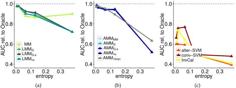
4.9 Experiments . . . 63
4.9.1 Algorithms . . . 63
4.9.2 Simulated domains . . . 64
4.9.3 UCI domains . . . 65
4.10 Discussion . . . 66
4.11 Appendix: proofs . . . 69
4.11.1 Proof of Lemma 35 . . . 69
4.11.2 Proof of Theorem 36 . . . 69
4.11.3 Proof of Lemma 37 . . . 71
4.11.4 Proof of Lemma 38 . . . 74
4.11.5 Proof of lemma 39 . . . 77
4.11.6 Proof of Theorem 41 . . . 78
4.11.7 Proof of Lemma 42 . . . 80
4.11.8 Proof of Theorem 43 . . . 81
4.11.9 Proof of Theorem 46 . . . 83
4.11.9.1 Proof of Equation 4.33 . . . 83
4.11.9.2 Proof of Equation 4.34 . . . 89
4.12 Appendix: additional experimental results . . . 90
4.12.1 Simulated domain for violation of homogeneity assumption . . 90
4.12.2 Additional tests on alter-∝SVM Yu et al. [2013] . . . 90
4.12.3 Scalability . . . 91
4.12.4 Full results on small domains . . . 92
4.13 References . . . 102
Contents ix
5 Learning with noisy labels I: theory for linear models 105
5.1 Motivation . . . 105
5.2 Learning setting . . . 106
5.3 Estimating the sufficient statistic andµSGD . . . 106
5.4 Generalization bounds . . . 107
5.5 Experiments . . . 110
5.6 Discussion . . . 111
5.7 Appendix: proofs . . . 114
5.7.1 Proof of Theorem 52 . . . 114
5.7.2 Proof of Theorem 53 . . . 114
5.7.3 Proof of Theorem 56 . . . 116
5.7.4 Proof of Corollaries 57 and 58 . . . 117
5.8 References . . . 118
6 Learning with noisy labels II: deep neural networks, multi-class, noise esti-mation 119 6.1 Motivation . . . 119
6.2 Learning setting . . . 120
6.3 Loss correction procedures . . . 122
6.3.1 The backward correction . . . 122
6.3.2 The forward correction . . . 122
6.3.3 Estimating the noise rates . . . 124
6.4 Noise free Hessians via ReLU . . . 125
6.5 Experiments . . . 126
6.5.1 Loss corrections withTknown or estimated . . . 126
6.5.2 Comparing with other loss functions . . . 128
6.5.3 Experiments on Clothing1M . . . 129
6.6 Discussion . . . 130
6.7 Appendix: proofs . . . 133
6.7.1 Proof of Theorem 60 . . . 133
6.7.2 Proof of Theorem 62 . . . 133
6.7.3 Proof of Theorem 63 . . . 133
6.7.4 Proof of Theorem 64 . . . 134
6.8 References . . . 134
7 Learning from vertically distributed data without entity matching 137 7.1 Motivation . . . 137
7.1.1 Entity resolution . . . 138
7.2 Learning setting . . . 139
7.3 Rademacher observations . . . 141
7.4 Building and learning from block rados . . . 143
7.4.1 Computation and optimality of block rados . . . 145
7.4.2 Learning from all block rados . . . 145
7.5 Experiments . . . 146
7.5.1 Domain generation . . . 147
7.5.2 Metric . . . 147
7.5.3 Results . . . 148
7.6 Discussion and references . . . 150
7.7 Appendix: proofs . . . 153
7.7.1 Proof of Theorem 68 . . . 153
7.7.2 Proof of Lemma 69 . . . 153
7.7.3 Proof of Theorem 72 . . . 153
7.7.4 Proof of Theorem 73 . . . 154
7.8 Appendix: extension to the more general setting . . . 154
7.9 Appendix: additional experimental results . . . 157
Chapter1
Introduction
1
.
1
Thesis summary
Supervised learning is by far the most effective application of the machine learning paradigm. However, its success in modern real word challenges is undermined by the fundamental assumption that we have perfect knowledge of the target variable, the label, at training time. Despite the unprecedented pace of accumulation of digital datasets,labeled datais still rare, due to several reasons: supervision is often generated by costly human annotation; relevant information may be obfuscated by privacy mechanisms; or, merely, labels are only known at a higher level of instance/temporal granularity with the respect to the one required for training. In addition to those issues, data collection is affected by ubiquitous noise corruption of various nature and therefore supervision is never perfectly reliable. As a consequence, learning is often performed with sparse, aggregated-level and/or noisy training labels. We consider all those scenarios all under the name ofweakly supervised learning.
In this Thesis, we approach this generic learning problem through the lens of Statistics and Learning Theory. Our solution is problem-agnostic yet constructive and it boils down to a simple two-steps procedure. First, estimate a sufficient statistic of the unknown labels from weak supervision; this quantity is calledmean operator. Second, plug the estimate into a standard loss function and learn the model by any gradient-based solver. The key to the second step is the definition of a family of losses that we call linear-odd. Its elements can be computed without the need of any label, given their sufficient statistic, by virtue of what we termloss factorization. Several commonly used losses belong to the family, e.g. logistic and square. From the theoretical viewpoint, linear-odd losses shed new light on generalization bounds with Rademacher complexity: the contribution of the supervision is isolated into one single term, which accounts for the deviation of the sufficient statistic from its population mean. From the algorithmic viewpoint, we bypass the need of estimating actual labels and therefore circumvent the difficult bi-convex optimization problem arising from naïvely modeling labels as latent variables. To put this into practice, a well-behaved estimator of the sufficient statistic remains to be defined. This is achieved depending on the particular nature of the weak supervision and relative assumptions.
We study in detail three scenarios of weak supervision. The first is calledlearning
from label proportions, where nothing is known about the target variable but its pro-portion over subsets of the training set, the bags. This setting is inspired by several applications where individual labels are not available, but ratios and percents are easy to estimate for domain experts, or given by other sources in terms of aggre-gates, e.g.surveys, census data. Despite the poor label knowledge, it is possible to learn linear classifiers with strong theoretical guarantees and good practical perfor-mance. We work under a weak distinguish-ability assumption of bags, which relaxes a similar but stricter condition in literature. In light of our two-step framework, the problem is reduced to estimating the mean operator from the label proportions. We do so by least square minimization with a manifold regularizer, which expresses our geometrical assumption on the data. A finite sample guarantee is given: the estima-tor is all the better as the maximum feature vecestima-tors norm increases. We name this algorithm the Laplacian Mean Map (LMM): after estimation, a standard loss function computed with the mean operator is minimized. The model output of LMM enjoys a data dependent approximation bound with respect to an ideal classifier learned with full supervision.
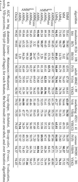
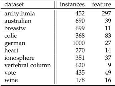
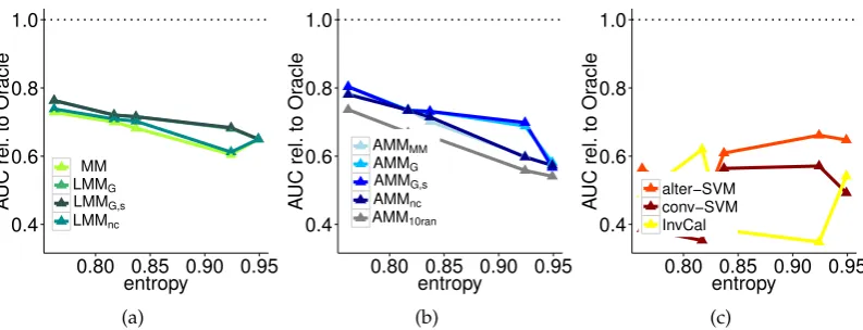
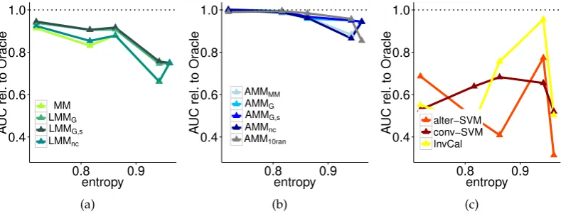
We then propose an iterative algorithm, the Alternating Mean Map (AMM). It takes the solution of LMM as input and optimizes it further over the set of label-ings consistent with the proportions, implementing coordinate descent minimization. This simple idea can highly improve the quality of the final model in practice, yet it does not suffer some of the drawbacks of the popular bi-convex iterative optimiza-tion. In fact, the LMM initializer performs significantly better than random vectors and is deterministic by definition. Moreover, computing the latent labels that match with the proportions while minimizing the loss can be efficiently done via sorting. Finally, we also formulate a specialized uniform convergence bound, involving a generalization of Rademacher complexity for learning from label proportions. The result includes a bag-wise surrogate risk for which we show that AMM optimizes a tractable bound. We experiment on UCI domains with up to hundreds of thou-sands of examples, comparing the algorithms to previous work. We simulate bags and their label proportions and retain labels for test set performance. Results display that AMM and LMM outperform the state of the art and sometimes even compete with the fully supervised learner, while requiring few proportions only. Tests on the largest domains display the scalability of both algorithms.
§1.1 Thesis summary 3
ideal model and ours cannot be arbitrarily large and the bound is data dependent by the mean operator. On the algorithmic side, we show how to adapt stochastic gra-dient descent and proximal algorithms to handle weak supervision. Once the mean operator has been estimated, the modification only requires a change of inputs and to sum up the mean operator to the model update. The theory is validated with ex-periments on UCI domains, on which we inject artificial noise. We assume to know the noise rates for the first step of estimation. Our approach of loss correction is effective: we obtain a significant gain in performance with respect to standard loss minimization with the same algorithm. Interestingly, in the presence of very high noise (one noise rate close to 50%) we still obtain sensible models, while learning with no loss correction often results in random guessing.
We study further the asymmetric label noise setting and consider multi-class clas-sification with deep neural networks, including recurrent neural networks. Once more, the only component we operate on is the loss function, thus our solution is ac-tually independent from any chosen architecture. Although, with neural networks, our two-step learning procedure requires more care. Here the sufficient statistic is computed upon intermediate feature representations that need to be learned and therefore cannot be estimateda priori. Still, even with multiple classes, what is suffi-cient for loss correction is the probability of flipping each class into any other, namely a transition matrix. Given the matrix, we propose two types of loss corrections; one follows the extension of the above idea to multi-class, the other is instead inspired by prior work on robust Deep Learning. Both corrections amounts at most to one inversion and multiplication of the noise matrix. Therefore, we show how to com-pute the noise rates from (noisy) data as the first step of learning. In particular, we adapt a recently published technique for noise estimation to the multi-class scenario. The whole learning process is summarized as follows: train the chosen neural net-work with standard loss using corrupted labels; exploit it to estimate the transition matrix; finally re-train the network with the corrected loss. Experiments on MNIST, IMDB, CIFAR-10, CIFAR-100 and a large scale dataset of clothing images show that a diversity of architectures — stacking dense, convolutional, pooling, dropout, batch normalization, word embedding, LSTM and residual layers — demonstrate noise ro-bustness for image recognition and sentiment analysis. Incidentally, we also prove that, when ReLU is the only non-linearity, the loss curvature is immune to label noise.
Finally, we explore an extension of the framework to the challenging problem of
learning from distributed datasets, where examples are “vertically” (feature-wise)
and some of the features are shared between the two domains. This can be seen as a peculiar setting of weakly supervised learning, since the mapping between each feature vector and relative label (although known) is effectively missing.
Traditionally, the problem would be approached by first solving (approximate) entity matching and subsequently learning the classifier in a standard manner. In-stead, following the underlying philosophy of the Thesis, we bypass the problem of estimating the unknown variables and look for sufficient statistics. In this setting, we require a different sort of loss factorization, expressed by the recently introduced concept of Rademacher observations (rados). Those statistics closely related to the mean operator and indeed can be thought as sufficient for subsets of examples — not just for labels — in the data. We replace the minimization of a loss over examples, which requires entity resolution, by theequivalentminimization of a loss over rados. In general, the number of rados is exponential in the sample size. We show that a large subset of these rados does not require to perform entity matching and can be easily obtained linking together partial views of examples with the same value of shared features. With a focus on square loss, we prove that optimization on those rados has time and space complexities smaller than the algorithm minimizing the equivalent square loss on examples. Last, we relax the key assumption that the data is vertically partitioned among peers — in this case, we would not even know the existence of a solution to entity resolution. In this more general setting, experiments support the possibility of beating the optimal peer in hindsight.
1
.
2
Organization and originality
§1.3 First-author publications included in the Thesis 5
1
.
3
First-author publications included in the Thesis
Patrini, G.; Nock, R.; Rivera, P.; and Caetano, T., (Almost) no label no cry. In NIPS, 2014.
Patrini, G.; Nielsen, F.; Nock, R.; and Carioni, M., Loss factorization, weakly
supervised learning and label noise robustness. InICML, 2016.
Patrini, G.; Nock, R.; Hardy, S.; and Caetano, T., Fast learning from distributed
datasets without entity matching. InIJCAI, 2016.
Patrini, G.; Rozza, A.; Menon, A.; Nock, R.; and Qu, L., Making deep neural
networks robust to label noise: a loss correction approach. Submitted to CVPR, 2017.
1
.
4
Contributed publications
Nock, R.; Patrini, G.; and Friedman, A., Rademacher observations, private data
and boosting. InICML, 2015.
Muzellec, B.; Nock, R.; Patrini, G.; and Nielsen, F., Tsallis regularized optimal
Chapter2
Background
The Chapter recalls basic notions of supervised Machine Learning, Learning Theory and Statistics, and presents a critical review of weakly supervised learning as tackled by prior work. Notations, formal statements and proofs of this introductory material are loosely inspired by the book of Shalev-Shwartz and Ben-David [2014].
2
.
1
Preliminary notation
We begin by defining some notation that will be used throughout the Thesis. R+ is the set of non-negative real numbers. For anym∈N, the sequence of positive natural number up to m is[m] =. {1, . . . ,m}. Boldfaces like v indicate (column) vectors; vi
(boldface) is theith element of a sequence of vectors instead;vi may either be theith
component of vector v or the ith element of a sequence of scalars {v1,v2, . . .}. 1 is the vector of all ones, with size determined by context, andei is the indicator vector,
that is 1 only at theith position.
Capital letters like A can indicate matrices, or sometimes constants scalar, de-pending on the context; Ai· and A·j are respectively rowi∈ [m]and column j∈ [n]
of matrix A ∈ Rm×n. 0 is either a vector or a matrix filled with zeros, with size
determined by context. I is the identity matrix. diag(v)is diagonal matrix withvon the diagonal. tr(A)is the trace of matrixA.
For any function f : R → R, we denote its first derivative at x by f0(x); the subdifferential set, that is, the set of all subdifferentials at point x is denoted by
∂f(x). For vector functions f :Rd →R, we indicate gradient at pointxby∇f(x).
We denote with 1{p} the indicator function of a predicate p, which is 1 when
true. [v]+ is max(0,v), for any scalar v. Inner products are written by angular
bracketsh·,·i. Sets and sequences are italic capital letter likeS. The probability of an event is denoted byP(·). The expectation over a distribution D is denoted asED[·]; the same notation is for empirical averages on a sampleS asES[·]=. 1/|S|∑· . We also refer to the setΣm =. {−1, 1}m, them-times Cartesian product of{−1, 1}.
2
.
2
The supervised learning problem
In Supervised Machine Learning we learn a map between two spaces by looking at examples. Learning Theory studies the role of those objects within the process of learning. Let setX be the input space setY the output space. Elementsx ∈ X ⊆Rd
are calledfeature vectors, observationsorinstancesand elementsy∈ Y are calledlabels. The function h : X → Y, named hypothesis or model, belongs to a hypothesis space H. Any pair(x,y)∈ X × Y is an example.
It is usual to frame the problem of learning in the language of probability. We assume that examples are drawn i.i.d from an unknown but fixed distribution D.
A (learning) sample S of size m is a finite sequence of examples {(xi,yi),i ∈ [m]}.
Notice that despite the commonly used “set-like” notation,S is actually a sequence, which in particular implies that examples can be repeated. At the same time, since examples are drawn i.i.d., their order does not strictly matter, except sometimes for notational convenience in defining algorithms. In regression, the output space is the real line, i.e.Y = R. In classification, the output space is instead discrete and labels are also calledclasses. For instance in binary classification, a main focus of this work, it is common to represent the output variable as taking values in{−1, 1}.
The goal of supervised learning is to find a hypothesis that generalizes well on unseen examples. Thus we first ought to define what is the quality measure for hypotheses. In classification, we refer to thegeneralization error, orrisk, the average number of labels correctly predicted by the model: ED 1{h(x) = y}. We could therefore define alearneras any algorithm minimizing the generalization error as:
h? =. argmin
h:X →Y
ED 1{h(x)6=y} (2.1)
The minimizer of this problem is called Bayes optimal and its risk is the Bayes risk. This formulation is problematic for several reasons. First, we have mentioned that the distributionDis unknown to the learner. Learning can only make use of the sample S, which provides an empirical version of the objective of Equation 2.1, namely the
empirical risk ES 1{h(x) 6= y}. Second, we need to define what the model space H
is. The choice of the model space is crucial for the success of learning, as discussed below. For most of the Thesis we consider one of the simplest hypothesis space, i.e.
the set of linear classifiers. To make this explicit, we will denote the model by a vector
θ ∈ Rd as h(·) =. hθ,·i. This often allows to simplify formal arguments while still
capturing essential properties. We introduce more complex model spaces in Chapter 6, that deals with deep neural networks, and Chapter 3, which briefly touches on non-parametric kernel methods. Third, in practice it would be difficult to optimize directly the error function, which is discontinuous and non-convex. Instead, it is common to resort to surrogate objectives calledloss functions.
A loss`:X × Y × H →Rmeasures the disagreement between labels and model predictions, although not necessarily by strict inequality, e.g. logistic and square losses (in formulae given below). By extension from the empirical risk, we call
§2.3 Learning Theory 9
We denote `-risks and empirical counterparts by RD,`(h) and RS,`(h) respectively.
The error itself can be thought as the risk a certain loss function, the 0/1 loss,
`01 = 1{yh(x) < 0}. As a result, we now formulate the empirical risk minimization
(ERM) framework, a fundamental paradigm in Machine Learning: argmin
h∈H
RS,`(h) (2.2)
One final important issue is hidden in the ERM formulation, that of overfitting. By searching for a modelin the learning sample, we may end up learning all too well particular variations of S, but with no guarantee that the model may generalize on unseen examples of D. Intuitively, when the size of the learning sample is small relatively to the model complexity, the model could memorize the whole sample itself, and overfitting is a potential threat. When obtaining more data for learning is not an option, overfitting can be combatted in several ways. We may replace the hypothesis spaceHwith one containing model with smaller capacity; or equivalently, we may express a “preference” over the elements ofHby balancing the empirical risk with an additional term acting as a regularizerΩ:H →R+. We update the learning framework of Equation 2.2 to thestructural risk minimizationto:
argmin
h∈H
RS,`(h) +λ·Ω(h) (2.3)
with λ > 0 balancing the two contributions. As we show below, Ωmay also be a
function of on the learning sample, depending on the kind of prior knowledge one needs to express in the problem.
2
.
3
Learning Theory
Loss functions have been studied extensively in the Machine Learning and Statistics literature. It is common to assume some preconditions for defining losses that are amenable of study: non-negativity and convexity are definitely the most widely re-quired. In our work, we do not strictly work under those conditions but we will make it explicit when particular results require them. Here we limit ourself to recall some definitions and properties that are relevant for what is discussed in the Thesis.
One first important requirement for loss functions isproperness. Definition 1. A loss`(y,h(x))isproperwhen:
argmin
h
Ey∼p(y|x)`(y,h(x)) =p(y|x) . (2.4)
This requirement states that the optimal model should be the conditional prob-ability of the class, given the observation. This way, models fitted via proper losses are actual probability estimators for the class.
−2 −1 0 1 2 −10
2 4 6
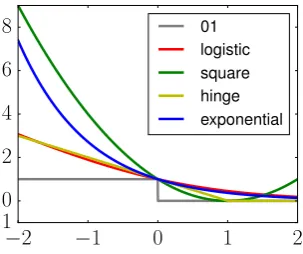
[image:20.595.205.357.113.240.2]8 01 logistic square hinge exponential
Figure 2.1: Losses as function of x = yh(x). Logistic is scaled by 1/ log(2)to be an upper bound of 01 loss, which is irrelevant for optimization.
functions calledmargin losses.
Definition 2. Amargin lossis defined as `(yh(x))=. `(x,y,h).
When clear by the context, we simply use a generic scalar argument `(x). Margin losses are implicitlysymmetric since`(yh(x))) =`(−y·(−h(x))). Examples are 0/1 loss 1{x < 0}, square loss (1−x)2, logistic loss log(1+e−x) (logistic regression), hinge loss[1−x]+(SVM) and exponential losse−x(boosting). Figure 2.1 shows how these losses are all designed to be upper bounds of 0/1 loss, a sensible strategy for optimizing the quantity that we ultimately wish to minimize. Among those margin losses, it is well known that hinge loss is not proper and cannot naturally be used as a class probability estimator [Platt, 1999].
Sometimes we will consider losses that are strongly convex functions, which is a common assumption to facilitate the derivation of desired upper bounds.
Definition 3. Letγ > 0. A differentiable function f(x) is γ-strongly convex if for any
x,x0 ∈Dom(f)we have:
f(x)− f(x0)≥ h∇f(x0),x−x0i+ γ 2
x−x022 . (2.5)
Similarly, it is common to refer to L-Lipschitzfunctions, that are such that|f(x)− f(x0)| ≤ Lkx−x0k for any x,x0. A comprehensive discussion on loss functions for binary classification is Reid and Williamson [2010].
2.3.1 Generalization bounds and Rademacher complexity
§2.3 Learning Theory 11
Definition 4. Letσ be a random variable drawni.i.d. from{±1}with uniform probability. Theempirical Rademacher complexityof a hypothesis space H with regard to sampleS
of size m and loss`is:
R(`◦ H ◦ S)=. Eσ∼Σm
"
1
msuph∈H
m
∑
i=1
σi `(yih(xi))
#
, (2.6)
while its population version R(`◦ H) =. ES∼D R(`◦ H ◦ S) is the Rademacher
com-plexity.
We recall two types of bound that we will use in the Thesis. For the sake of com-pleteness, we prove them in the Appendix of this Chapter; proofs rely heavily on the application of McDiarmid’s inequality [McDiarmid, 1998].
Theorem 5. Assume a bounded loss, i.e. |`(x)| ≤ C,∀x. Then for any δ ∈ (0, 1), with
probability at least1−δover the choice ofS, simultaneously for all h∈ H, we have:
RD,`(h)−RS,`(h)≤2R(`◦ H) +C
r
2
mlog
1
δ . (2.7)
Moreover, let the empirical risk minimizer be hˆ = argminh∈HRS,`(h). For anyδ ∈ (0, 1),
with probability least1−δ over the choice ofS, we have:
RD,`(hˆ)− inf
h∈HRD,`(h)≤4R(`◦ H) +2C
r
2
mlog
1
δ . (2.8)
Proof in 2.6.1. This first inequality limits the difference between risk and its empirical approximation; this probabilistic guarantee corroborates the idea of fitting the model on a finite but not too small sample S. The second is a bound on the
excess `-risk, that is the difference between the risk of ERM model and the smallest
risk achievable for models in H, the second being unavoidable even for known D. Those bounds have a typical shape often encountered in generalization results. Two terms contribute to their significance. The Rademacher complexity quantifies the capacity of the model space H of fitting all possible label assignments. While large capacity means better approximation and therefore lower empirical risk, this is not necessarily good for generalization risk on D. In fact, low Rademacher complexity tightens the bounds. This is along the line of the classic results on the VC-dimension, which is indeed an upper bound of the Rademacher complexity. The remaining term is a statistical penalty due to requiring uniform convergence. The bound holds true for anyS, and in particular for samples not being much representative ofD, that is, drawn from areas with low probability mass on the support ofD. This is the role of
δ in the probability inequality, while largem weights down the possibility of those
bad choices ofS.
be the fastest rate achievable in learning [Vapnik, 1998]. Those improved guarantees will not be discussed in the Thesis.
Next, we specialize some of the previous results for Lipschitz loss functions and linear classifiers.
Lemma 6. Let`be a L-Lipschitz function. Then: R(`◦ H)≤ LR(H), where:
R(H)=. ES∼DEσ∼Σm
"
1
msuph∈H
m
∑
i=1
σi h(xi)
#
, (2.9)
The result is also helpful to clarify what the Rademacher complexity computes: it measures the capacity of hypotheses inHby the supremum of correlation with ran-dom noise — the ranran-dom variableσ. We will refer to bothR(H)andR(`◦ H)(with
dependency on `) as Rademacher complexity. Second, we can give generalization bounds specialized for linear classifiers.
Theorem 7. Let X be a vector space such that X = {x : kxk2 ≤ X < ∞}. Let H
be the space of bounded linear classifiers H = {θ : kθk2 ≤ H < ∞}. Assume a
L-Lipschitz, bounded loss|`(x)| ≤ C,∀x. With probability at least1−δ over the choice ofS,
simultaneously for all h∈ H, we have:
RD,`(h)−RS,`(h)≤
2LXH √
m +C
r
2
mlog
1
δ . (2.10)
Moreover, let the empirical risk minimizer be hˆ = argminh∈HRS,`(h). For anyδ ∈ (0, 1),
with probability least1−δ over the choice ofS, we have:
RD,`(hˆ)− inf
h∈HRD,`(h)≤
4LXH √
m +2C
r
2
mlog
1
δ . (2.11)
Proof in 2.6.2. Finally, we have mentioned that Rademacher complexity is a data dependent measure. Although, previous results account for its population mean, not the empirical complexity. Yet it is simple to show that the empirical Rademacher complexity converges rapidly to its population mean by applying McDiarmid’s in-equality.
Lemma 8. Assume a bounded loss,i.e.|`(x)| ≤C,∀x. Letδ >0. We have with probability
1−δ:
|R(`◦ H)− R(`◦ H ◦ S)| ≤C
r
2
mlog
2
δ . (2.12)
§2.4 Maximum likelihood, exponential family and sufficient statistics 13
2.3.2 Calibrated losses
The generalization bounds above express uniform convergence guarantees of the ERM with respect to the surrogate loss function chosen for learning. Ultimately, we wish to obtain similar bounds for the error, which is the measure of goodness of the hypothesis. To that objective, we define a subclass of margin losses called
calibrated [Bartlett et al., 2006], which transforms the previous results in bounds for
the generalization error. We introduce them by a sufficient and necessary condition for the case of convex losses.
Definition 9. Let ` be a non-negative convex loss. ` is (classification) calibratedif and only if`is differentiable in0and`0(0)<0.
Theorem 10. Let ` be calibrated. Then, there exists a convex, non-decreasing, invertible
functionψ` :[0, 1]→R+, withψ`(0) =0, such that for any h∈ H:
ψ`
RD,0/1(h)−inf
h RD,0/1(h)
≤RD,`(h)−inf
h RD,`(h) . (2.13)
It follows that any time we can prove a bound for the excess`-risk, we immediately translate it to the error viaψ−`1. For connections between proper and calibrated losses
see Reid and Williamson [2010].
2
.
4
Maximum likelihood, exponential family and sufficient
statistics
So far we have seen learning within ERM. An alternative set up for learning prob-lems is the notion of maximum likelihood estimation (MLE), a classic procedure for fitting models in Statistics. We start by assuming that our model belongs to a certain parametric probability distribution. Learning is then accomplished by fitting those parameters to the data by maximizing its likelihood. In particular, we can learn a binary classifier in the conditional (binary) exponential family parameterized by a vectorθ∈Rd:
pθ(y|x) =exp hθ,yxi −log
∑
y∈Y
exphθ,yxi
!
(2.14)
Here, yis the only random variable. The two terms in the exponent are the log-partition function, which normalizes the distribution such that it can sum to one, and the inner product between parameters and the sufficient statistic yx. Under the
exponential family as:
argmax θ
m
∏
i=1
exp hθ,yixii −log
∑
y∈Yexphθ,yxii
!
= (2.15)
argmax θ
exp
m
∑
i=1
hθ,yixii − m
∑
i=1 log
∑
y∈Y
exphθ,yxii
!
. (2.16)
By taking log and a negation, the objective of 2.16 becomes:
m
∑
i=1 log
∑
y∈Y
exphθ,yxii − m
∑
i=1
hθ,yixii (2.17)
=
m
∑
i=1 log
∑
y∈Y
exphθ,yxii − m
∑
i=1
log exphθ,yixii (2.18)
=
m
∑
i=1
logexphθ,xii+exphθ,−xii exphθ,yixii
(2.19)
=
m
∑
i=1
log(1+exp(−2yihθ,xii)) . (2.20)
Step 2.20 is true since y ∈ {±1}. Finally, by re-parameterizing θand normalizing,
we obtain logistic loss. These steps prove how the two approaches for learning, ERM and MLE, are equivalent for conditional exponential family and logistic loss. Addi-tionally, Equation 2.17 shows how the loss splits into a linear term aggregating the labels sufficient statistics and another, label free term. We consider this equivalence between conditional exponential family and logistic loss as common knowledge (in spite of being unaware of any published material). One of the key theoretical contri-bution of the Thesis is to demonstrate how this is not a coincidence: we will introduce a broad new family of losses for which this decomposition is always valid.
2.4.1 Sufficient statistics
Why did we call the quantities yx and∑iyixi sufficient statistics? A statistic is any
function g computed from a sample S. Intuitively, a statistic g(S)is sufficient (for the parameter θ) when it aggregates all information of S, such that no better model
could be learned from S in place of g. We are mostly interested in sufficiency with regard toy, thus we will only look into this case. In formulas, a statisticgis sufficient forθwith respect to any random variableYwith outcomeyif:
P(θ|y) =P(θ|g(y)),∀y∼Y . (2.21)
We provide an equivalent definition that, although somewhat less intuitive, is useful for conceiving some formal results in the Thesis.
§2.5 Weakly supervised learning 15
forθ with regard to Y when for each pair of outcomes y,y0 of Y we have:
P(θ|g(y))
P(θ|g(y0)) does not depend on y⇔ g(y) =g(y
0) . (2.22)
An additional equivalent characterization for sufficient statistics is provided by the classic Fisher-Neyman Theorem [Lehmann and Casella, 1998].
Theorem 12(Fisher-Neyman). Let pθ(y)be the probability density function of y. Then g
is sufficient for θif and only if two non-negative functions p(i) and p(ii) can be found such
that:
pθ(y) = p (i)
θ (g(y))·p (ii)(
y) . (2.23)
In other words, the probability density factors in two functions, such that θ
inter-acts with the y only through g. This can be used to show that yx is indeed suffi-cient for θwith regard toy in the case of the conditional exponential family
(Equa-tion 2.14). It holds that p(ii)(y|x) = 1, g(y|x) = yx and p(i)
θ (·|x) = exp(hθ,·i − log∑y∈Yexp(hθ,yxi), since the value ofyis not needed for computing p(θi).
2
.
5
Weakly supervised learning
This Section is halfway between an informal problem statement and a high level lit-erature review for weakly supervised learning problems and relative frameworks for solutions. “Weakly supervised learning” is a non-standard yet widely used termi-nology to describe scenarios that sit somewhere in between of supervised and unsu-pervised learning; other literature refers to, for instance, indirect [Raghunathan et al., 2016] or distant supervision [Mintz et al., 2009; Surdeanu et al., 2012]. This class of learning problems relaxes one fundamental assumption of supervised learning: the learner does not have perfect labels, that is, there is no guarantee that each label is fully observable and that each observed label is free from mistakes. This informal definition is deliberately vague as it is meant to encompass a large diversity of learn-ing settlearn-ings. For example, labels may be misslearn-ing as with semi-supervision[Chapelle et al., 2006] and positive and unlabeled data [du Plessis et al., 2015], noisy [Natarajan et al., 2013], aggregated as it happens in multiple instance learning [Dietterich et al., 1997] and learning from label proportions [Kuck and de Freitas, 2005], or given in a candidate set which include the only correct one, as in partial labelsor superset label
learning [Cour et al., 2011; Liu and Dietterich, 2014]. We also stress the fact that all
these problems share the same objective of supervised learning, which is learning a classifier — or occasionally a regressor —, in contrast with “fully unsupervised” learning.
Formally, we model a weakly supervised problem by a corruption process that takes the original distribution D and produces a corrupted distribution De, from which we get a corrupted sampleSe:
D −−−→corrupt De −−−→sample Se (2.24)
A fundamental assumption is that the marginal distribution of the features is un-touched by corruption, that is, PD(x) = PDe(x). This is all the formalism we need but we give more concrete examples ofSefor some particular cases.
Example. In semi-supervised learning, the learner sees two subsamples, one fully labeled and the other unlabeled: Se = (SL,SU), with SL = {(xi,yi),i ∈ [mL]} and
SU = {xi,i ∈ [mU]}. In positive and unlabeled learning, the scenario is similar but
the labeled examples are always positiveSL ={(xi, 1),i∈ [mL]}.
Example. When labels are noisy, it is usually assumed that the learner sees them all, although without guarantees of their truthfulness. Hence, Se = {(xi, ˜yi),i ∈ [m]},
where ˜yis drawn from some corrupted label distribution p(y˜).
Example. It is less obvious how to formalize supervision given at aggregate level; a possible choice is the following. Let us consider the original learning sample given by two ordered sets, one containing observations and the other one the relative la-bels: S = (SX,SY); observations are mapped to respective labels by indices. The
corrupted sample leaves features vectors untouched us usual, yet it partitions them
inton bags as SX = Sj∈[n]Sj with ∀j,j0 Sj∩ Sj0 = ∅. A certain type of supervision
is defined at the level of bags by π ∈ Rn. The resulting corrupted sample is then
e
S = ({Sj}j∈[n],{πj}j∈[n]). In learning from label proportions, πj ∈ [0, 1] represents
the fraction of positive labels for each bag j. In multiple instance labels, the supervi-sion is even weaker andπj ∈ {0, 1}is 1 if at least one label in bag jis positive1.
The difference between those learning settings is not crisp, for two reasons. On one hand, it is plausible that they can be combined by mixing the types of corruption. For instance, we can easily imagine that some labels are missing but those known are noisy; another common scenario is semi-supervised learning with additional prior knowledge on large unlabeled data, e.g. as in Bilenko et al. [2004]. On the other hand, some learning settings can be thought to be more general than others, without a total ordering in a hierarchy. For instance, the noisy label distributionp(y˜)may be modeling the event of “label suppression” so as to encompass missing labels as well [Menon et al., 2015]; multiple instance learning can be thought as a particular, less informative supervision with respecting to label proportions [Kuck and de Freitas, 2005]; at the same time, algorithms for semi-supervised learning have been shown to be apt for multiple instance learning [Zhou and Xu, 2007].
1Other encodings of supervision of MIL have been formalized. Also, MIL is sometimes intended as
§2.5 Weakly supervised learning 17
2.5.1 Empirical risk minimization under weak supervision
What is the meaning of computing the empirical risk on the corrupted sample,
RSe,`(h)? By relaxing the assumption of “full supervision” the framework of ERM loses its sense. Depending on the nature of weak supervision, this quantity may be computable either only partially (semi-supervision) or completely but with lit-tle meaning (noisy labels); worse, when supervision is given at multi-instance level, there exists no obvious way to estimate the risk. Mathematically, the problem of searching for risk minimizer becomes ill-posed. We discuss a non-exhaustive overview of families of methods proposed in the past.
Case (i): some observations have individual labels, but some others do not. We adopt the definition of Se= SL∪ SU of semi-supervised learning for simplicity. We can formulate an optimization problem such as:
argmin
h∈H
RSL,`(h) +λ·reg(Se,h) (2.25)
The regularizer is intended to exploit the information of the additional unlabeled features vectors to bias the search in the model space. The idea is that the feature geometry, regardless of unknown labels, should be informative about the class dis-tribution. Formally, one of three celebrated assumptions is required for this to be true: the smoothness, the cluster, or the manifold assumption [Chapelle et al., 2006];
the causal direction of data generation has also been taken into account for
justify-ing the success of semi-supervised learnjustify-ing [Janzjustify-ing et al., 2012]. Examples of this framework for learning with missing labels are: transductive SVM [Joachims, 1999], information regularization [Szummer and Jaakkola, 2002], label propagation as a regularizer [Zhu and Ghahramani, 2002; Bengio et al., 2006], entropy regularization [Grandvalet and Bengio, 2004], manifold regularization [Belkin et al., 2006], ladder network [Rasmus et al., 2015] and graph embedding [Weston et al., 2012; Yang et al., 2016].
Case (ii): noisy labels. Design a corrected loss ˜` satisfying a certain property of robustness with respect to the noise and minimize it instead of the original`:
argmin
h∈H
RSe,˜`(h) (2.26)
Often, the robust loss is either non-convex [Masnadi-Shirazi et al., 2010; Ding and Vishwanathan, 2010; Ghosh et al., 2015] or requires certain knowledge of the label corruption p(y˜|y)[Stempfel and Ralaivola, 2009; Natarajan et al., 2013], with the no-ticeable exception of the linear “unhinged” loss [van Rooyen et al., 2015].
modeling the unknown labels as latent variables. Although ultimately the learner output is a model, the estimation of the labels become a fundamental intermediate step for learning. This framework closely resembles and it is often implemented as the Expectation Maximization (EM) algorithm, sharing the well known drawbacks. Weak supervision helps the search in the model space by formulating constraints (hard of soft) to be satisfied by the model:
argmin
h∈H,y∈Y
R(SX,SY),`(h) +λ·constr(SX,SY,h) (2.27)
Examples of this approach are Yu et al. [2013] for LLP, Andrews et al. [2002] for MIL. This framework easily extends to the case of constraints on (functions of) features vectors, which may be loosely interpreted as weak supervision as well. In this line of work, particularly relevant for applications in NPL, constraints are enforced on particular features, such as the word “amazing” is a strong indicator of a highly rated movie review; a sample of those methods are constraint driven learning Chang et al. [2007], generalized expectation constraints Mann and McCallum [2008], poste-rior constraints Ganchev et al. [2010], and label regularization [Mann and McCallum, 2010; Ardehaly and Culotta, 2015]. A unifying framework of this kind of EM-based inference with constraints is elaborated by Samdani et al. [2012].
Case (iv): Prior work also attempts an agnostic treatment of weak supervision for ERM, as we envision in the Thesis. A broad, comparative formalization of weakly su-pervised problems is presented by Garcıa-Garcıa and Williamson [2011]. Joulin and Bach [2012] attack a version of the generic Problem 2.27 by a convex relaxation and a dedicated optimization algorithm based on semidefinite programming. Li et al. [2013] formulate a tighter and more scalable convex relaxation of a generic weakly supervised max-margin problem. Zantedeschi et al. [2016] propose the β-risk, a
sur-rogate risk augmented with a matrix parameter β which captures the reliability of
each instance label; models, labels and β are estimated iteratively. A last important
mention is the work of Raghunathan et al. [2016] that, due to the strong similarity with our framework, will be discussed in detail in Section 3.7 of the next Chapter.
§2.6 Appendix: proofs 19
(or action) and label (reward). As we do not study in any case neither sequential data nor interactive scenarios, or in other words, we always assume i.i.d. samples, those learning setting are as well outside the scope of the Thesis.
2
.
6
Appendix: proofs
2.6.1 Proof of Theorem5
The proof follows Shalev-Shwartz and Ben-David [2014]. Let us first recall McDi-armid’s inequality [McDiarmid, 1998].
Lemma 13. LetZ be a set and f :Zm→Rbe a function of m variables such that for some
c>0, for all i0 ∈[m]and for all z1, . . . ,zm,zi0 ∈ Z we have:
|f(z1, . . . ,zi, . . . ,zm)− f(z1, . . . ,zi0, . . . ,zm)| ≤c . (2.28)
Let now be Z1, . . . ,Zm m independent random variables taking values in Z. Then, with
probability at least1−δwe have:
f(Z1, . . . ,Zm)−E[f(Z1, . . . ,Zm)]≤c
r
m
2 log 1
δ . (2.29)
We also make use of an additional Lemma that connects Rademacher complexity with the maximum deviation of empirical risk from the respective risk.
Lemma 14. Letφ(S) =suph∈HRD,`(h)−RS,`(h). Then:
ED φ(S)≤2R(`◦ H) . (2.30)
For any bounded loss function |`(c)| ≤ C, the function φ satisfies McDiarmid’s
in-equality withc=2C/m. Therefore:
φ(S)≤ED φ(S) +C
r
2
mlog
1
δ ≤2R(`◦ H) +C
r
2
mlog
1
δ , (2.31)
with probability at least 1−δ. Clearly, for allh∈ H,RD,`(h)−RS,`(h)≤φ(S), which
proves the first statement. For the second statement, for any h? ∈ H, we write:
RD,`(hˆ)−RD,`(h?) =RD,`(hˆ) +
−RS,`(hˆ) +RS,`(hˆ)
+−RS,`(h?) +RS,`(h?)
−RD,`(h?) (2.32)
≤RD,`(hˆ)−RS,`(hˆ)
+RS,`(h?)−RD,`(h?)
(2.33)
≤2φ(S) (2.34)
2.6.2 Proof of Theorem7
We need to compute an upper bound of the Rademacher complexity for linear clas-sifiers.
Lemma 15. Let X be a vector space such that X = {x : kxk2 ≤ X < ∞}. LetH be the
space of bounded linear classifiersH ={θ:kθk2≤ H<∞}. Then:
R(H)≤ XH√
m . (2.35)
Proof
mR(H) =mED,σ sup
θ∈H 1
m
m
∑
i=1
σihθ,xii (2.36)
=ED,σ sup θ∈H
m
∑
i=1
σihθ,xii (2.37)
=ED,σ sup θ:kθk2≤B
m
∑
i=1
σihθ,xii (2.38)
=ED,σ sup θ:kθk2≤B
hθ,
m
∑
i=1
σixii (2.39)
≤ HED,σ
"
m
∑
i=1
σixi
2 # . (2.40)
The last Step is due to Cauchy-Schwartz inequality. Next, by Jensen’s inequality it holds: Eσ " m
∑
i=1
σixi
2 #
=Eσ
m
∑
i=1
σixi
2 2 1/2 ≤ Eσ
m
∑
i=1
σixi
2 2 1/2 . (2.41)
Finally, since the variablesσi are independent, we have:
Eσ m
∑
i=1
σixi
2 2 =Eσ
"
∑
i,j
σiσjhxi,xji
#
(2.42)
=
∑
i6=j
hxi,xjiEσ
σiσj+
m
∑
i=1
hxi,xiiEσ
σi2 (2.43)
=
m
∑
i=1
kxik22 (2.44)
§2.6 Appendix: proofs 21
Altogether we have:
mR(H)≤ HED mX21/2 =√mXH , (2.46) which proves the Lemma.
Chapter3
Weakly supervised learning and
loss factorization
We introduce a new family of loss functions called linear-odd for the formal study of weak supervision. The central result is the statement of the Loss Factorization Theorem that isolates the effect of supervision into a label sufficient statistic. As a result to this finding, we can formulate a generic two-step approach for solving weakly supervised problem, by calling standard supervised algorithms based on gradient descent. This Chapter is the most abstract and can be thought as a toolbox of formal results and meta-algorithms to be specialized for particular instances of weak supervision. The Chapter, if not the Thesis in a whole, is inspired by the popular quote:
“One should solve the problem directly and never solve a more general problem
as an intermediate step”[Vapnik, 1998].
3
.
1
Linear-odd losses and Loss Factorization
In Chapter 2 we shown that MLE of the exponential family is equivalent to ERM with logistic loss. In doing so, we proven that logistic loss decomposes into two terms, one of which is linear. We now give a name to that statistical object and show some intriguing properties connecting the idea of sufficiency from Statistics to Learning Theory.
Definition 16. The (empirical)mean operatorof a learning sampleS isµS =. ES[yx] .
In the following, we drop the dependency of S when clear by the context. The
name mean operator, or mean map, is borrowed from the theory of Hilbert space
embedding [Quadrianto et al., 2009]. In this Thesis, µwill play the role of sufficient
statistic for labels with regard to a set of losses. The next is motivated by Definition 11 by taking log-odd ratio.
Definition 17. A function T(S)is said to be a sufficient statistic for a variable y with regard
to a set of losses Land a hypothesis spaceH when for any` ∈ L, any h ∈ Hand any two
samplesS andS0 the empirical`-risk is such that1:
RS,`(h)−RS0,`(h)does not depend on y⇔T(S) =T(S0) . (3.1)
We will often call any such quantity a label sufficient statistic. We now state and prove one of the main theoretical contributions of the Thesis, the Loss Factoriza-tion Theorem – by reminiscence of Fisher-Neyman FactorizaFactoriza-tion Theorem 12. As a consequence, we establish sufficiency of mean operators for a large set of losses. Theorem 18 (Factorization). LetH be the space of linear hypotheses. Assume that a loss
` is such that`o(x) = (. `(x)−`(−x))/2is linear. Then, for any sampleS and hypothesis
h∈ Hthe empirical`-risk can be written as:
RS,`(h) =
1
2RS2x,`(h) +`o(h(µ)) , (3.2)
whereS2x =. {(xi,σ),i∈ [m],∀σ∈ Y}.
Proof We detail the proof as it clearly highlights the relevant elements allowing losses to factor. A key ingredient is an elementary fact from calculus: any function
writes (uniquely) as the sum of an even and an odd function. Therefore, we can write a
loss function`(x)as:
`(x) = 1
2[`(x) +`(−x) +`(x)−`(−x)] (3.3)
=`e(x) +`o(x) , (3.4)
where`e(x)=. 12[`(x) +`(−x)]and`o(x)=. 12[`(x)−`(−x)]are respectively an even
and an odd function (see also Figure 3.1). The empirical risk is:
RS,`(h) =ES[`(yh(x))] (3.5)
= 1 2ES
h
`(yh(x)) +`(−yh(x)) +`(yh(x))−`(−yh(x))i (3.6) = 1
2ES
h
∑
σ∈Y`(σh(x))i
+ESh`o(yh(x))i (3.7) = 1
2ES2x
h
`(σh(x))
i
+ESh`o(h(yx))
i
. (3.8)
Step 3.8 is due to the definition of S2x and linearity of h. Finally, exploiting the
properties of the loss assumed by the Theorem and the linearity of expectation, we
1Notice that the focus in the Definition is on the variabley(confront with Definition 11). This is
§3.1 Linear-odd losses and Loss Factorization 25
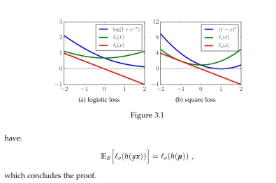
−2 −1 0 1 2
−1 0 1 2 3
log(1 +e−x) ℓe(x)
ℓo(x)
(a) logistic loss
−2 −1 0 1 2
−4 0 4 8 12
(1−x)2
ℓe(x)
ℓo(x)
[image:35.595.107.503.98.360.2](b) square loss
Figure 3.1
have:
ESh`o(h(yx))
i
=`o(h(µ)) , (3.9)
which concludes the proof.
Factorization splits`-risk in two parts. A first term is the`-risk computed on the
same losson the “doubled sample” S2x that contains each observation twice, labeled
with opposite signs, hence it does not require any label knowledge. A second term is a function`oofhapplied to the mean operatorµ, which aggregates all sample labels.
Also observe that `o is by construction an odd function,i.e. symmetric with respect to the origin. We call the losses satisfying the Theoremlinear-odd.
Definition 19(Linear-odd loss). A loss`is a-linear-odd(a-lol) when, for any a∈R:
`o(x) = (`(x)−`(−x))/2=ax . (3.10) Notice how this does not exclude losses that are smooth, convex, or non-proper. From now on, in this Chapter we considerH as the space linear hypotheses
h(·) =hθ,·i. As a consequence of Theorem 18,µis sufficient for all labels.
Corollary 20. The mean operatorµis a sufficient statistic for the label y with regard tolols
and the space of linear classifiersH.
Proof in 3.5.1. The practical consequence of this Corollary is at the core of the applications in the Thesis: the single vector µ ∈ Rd summarizes all information
concerning the linear relationship between y and x for losses that are lol. But
be-fore dealing with the theoretical and practical consequences, we discuss the natural question at this point: how restrictive is the linear-odd condition?
3.1.1 The extent of linear-odd losses
loss even function`e odd functionlo
generic `(x) 12(`(x) +`(−x)) 12(`(x)−`(−x))
lol `(x) 1
2(`(x) +`(−x)) ax
ρ-loss ρ|x| −ρx+1 ρ|x|+1 −ρx (ρ≥0)
unhinged 1−x 1 −x
perceptron max(0,−x) x sign(x) −x
double-hinge max(−x, 1/2 max(0, 1−x)) † −x spl al+l?(−x)/bl al+ 1
2bl(l?(x) +l?(−x)) −x/(2bl)
logistic log(1+e−x) 12log(2+ex+e−x) −x/2
square (1−x)2 1+x2 −2x
Matsushita √1+x2−x √1+x2 −x
Table 3.1: Factorization of losses. † for reason of space, the even part of double-hinge is written here as: max(−x, 1/2 max(0, 1−x)) +max(x, 1/2 max(0, 1+x)).
Example. For logistic loss it holds that (Figure 3.1a):
`o(x) = 1 2log
1+e−x
1+ex (3.11)
= 1 2log
e−x2(ex2 +e−x2) ex2(e−x2 +ex2)
(3.12) = −x
2 . (3.13)
Example. Unhinged loss `(x) = 1−x of van Rooyen et al. [2015], which is trivially linear-odd. Instead, the standard hinge loss `(x) = [1−x]+ does not factor in a linear term.
Example. Double-hinge and perceptron losses are proven to be linear-odd in du Plessis et al. [2015]. See also Appendix 3.6.5.
Example. The class of symmetric proper losses (spls) [Nock and Nielsen, 2009], e.g.
logistic, square and Matsushita losses, satisfies the linear-odd condition. Let φ be
permissible generator, i.e. φ is strictly convex, differentiable and symmetric with
respect to 1/2 and with dom(φ)⊇[0, 1]. spls are defined as`(x) =a φ+φ
?(
−x)/bφ,
whereφ? is the convex conjugate ofφ. Then, sinceφ?(−x) =φ?(x)−x, we have:
`o(x) = 1
2
aφ+
φ?(−x)
bφ
−aφ− φ?(x)
bφ
(3.14) = 1
2bφ
(φ?(x)−x−φ?(x)) (3.15)
=− x 2bφ
. (3.16)
§3.2 Generalization bounds 27
One may question whethersplandlolare equivalent. Table 3.1 gives an answer
in the negative already: there are examples of non-smooth functions that arelol. The
next result provides a more complete picture by giving an exhaustive characterization of the family of linear-odd losses.
Lemma 21. The exhaustive class of linear-odd losses is in 1-to-1 mapping with a proper
subclass of even functions,i.e.`(x) =`e(x) +ax, with`eany even function.
Proof in 3.5.2. Interestingly, the proposition also let us engineer losses that always factor: choose any even function`e with desired properties — it need not be convex nor smooth. The loss is then`(x) =`e(x) +ax, withato be chosen. For example, let `e(x) =ρ|x|+1, withρ>0. `(x) =`e(x)−ρxis alol; furthermore,`upper bounds
01 loss and intercepts it in`(0) =1. Non-convex`can be constructed similarly. Yet, not all non-differentiable losses can be crafted this way since they are notlol.
From the optimization viewpoint, we may want to keep properties of `after fac-torization. The good news is that we are dealing with the same` plus a linear term. Thus, if the property of interest is closed under summation with linear functions, then it will hold true. An example is convexity: if ` is lol and convex, so is the
factored loss. The same is true for differentiability.
In Appendix 3.6, we also elaborate on the relevance of the mean operator relating it to the covariance between x and y (Subsection 3.6.1), discuss the generality of Factorization beyond lols and linear models (Subsection 3.6.2) and state sufficient
and necessary conditions to bound other known losses, e.g. hinge and Huber, by
lols (Subsection 3.6.3).
3
.
2
Generalization bounds
A consequence of working withlols is on generalization bounds. We first derive an
improved upper bound to the Rademacher complexity ofHcomputed onS2x.
Lemma 22. Suppose m even. Suppose X = {x:kxk2≤ X}be the observations space, and
H = {θ : kθk2 ≤ H}be the space of linear hypotheses. Let Σ2m =. ×j∈[2m]Y. Then the
empirical Rademacher complexity:
R(H ◦ S2x)=. Eσ∼Σ2
"
sup θ∈H
1 2m
∑
i∈[2m]
σihθ,xii
#
(3.17)
ofHonS2xsatisfies:
R(H ◦ S2x) ≤ v·√XH
2m , (3.18)
with v=. 12+12
q
1 2−m1.
calculation of the complexity of a double sized sample by Lemma 15 would give a coefficient ofXH/√2m. Here we multiply it byv< (√2+1)/(2√2)≈0.85. This is relevant when combined into the next Theorem. The result sheds new light on excess
`-risk bounds on Rademacher complexity with linear hypotheses.
Theorem 23. Assume ` is a-lol and L-Lipschitz. Suppose Rd ⊇ X = {x : kxk2 ≤
X < ∞} and H = {θ : kθk2 ≤ H < ∞}. Let c(X,H) =. maxy∈Y`(yXH)and θˆ =.
argminθ∈HRS,`(θ). Then for anyδ >0, with probability at least1−δ:
RD,`(θˆ)−RD,`(θ?)≤ √
2+1 2 ·
XHL √
m +
c(X,H)·
s
1
mlog
1
δ
+2|a|H· kµD−µSk2 , (3.19)
or more explicitly:
RD,`(θˆ)−RD,`(θ?)≤ √
2+1
2 ·
XHL √
m +
c(X,H)·
s
1
mlog
2
δ
+2|a|XH·
s
d
mlog
2d
δ
. (3.20)
Proof in 3.5.4. The former expression displays the contribution of the non-linear part of the loss, keeping aside what is missing: a deviation of the empirical mean operator from its population mean. When µ is not known because of partial label
knowledge, the choice of any estimator would affect the bound only through that norm discrepancy. The second expression highlights the interplay of the two loss components. c(X,H)is the only non-linear term, which may well be predominant in the bound for fast-growing losses, e.g. strongly convex. Moreover, we confirm that the linear-odd part does not change the complexity and only affects the statistical penalty by a linear factor, with a dependency on d. We remark that we could as well obtain a bound in the shape of the first statement of Theorem 5; we opt for an excess-risk bound to compare easily with prior work in Chapter 5.
Linear-odd losses are also calibrated under mild conditions.
Lemma 24. Every a-linear-odd loss that is non-negative, convex, differentiable in0and with
a <0is calibrated.
Proof in 3.5.5. Consider again Table 3.1. Those losses are all convex and all have
a <0. They are also differentiable in 0 with the exception ofρ-loss and “perceptron”.
![Table 4.2: AUC on the toy dataset of Yu et al. [2013]](https://thumb-us.123doks.com/thumbv2/123dok_us/8115956.238218/75.595.240.398.112.215/table-auc-toy-dataset-yu-et-al.webp)