Development and demonstration of a diode laser sensor for a scramjet combustor

8. Interpretation of results

The temperature and water vapour concentration measured in a scramjet com-bustor were presented in the previous chapter. The measurements were able to resolve trends over the test time of the facility, showed that different condi-tions existed at different heights in the duct and were repeatable between shots. Nevertheless, since the temperature and water vapour concentration were de-rived from a line of sight measurement, it is not clear how well the measured temperature and concentration relate to the conditions present in the scramjet duct.

The purpose of this chapter is to establish whether or not the measurements are useful, given this limitation. This is done by comparison with other informa-tion sources. As part of this work, scramjet experiments were carried out with pressure transducer instrumentation, providing wall pressure data that can be compared with TDLAS results. Other experiments, documented by Stotz and O’Byrneet. al. [80, 111], usedOH–PLIF to visualise the location ofOHradicals near the cavity.

Since the different techniques provide different information, a direct compari-son is not possible. Instead, it is first shown how the techniques can be used in-dependently to determine the presence of combustion. Following this, pressure and TDLAS measurements are combined to obtain an estimate of the mixing ratio of water molecules.

Next, a situation where a direct comparison is possible is considered by compar-ison between TDLAS and computational fluid dynamics results, or CFD. CFD is able to predict the variability of the water and temperature along the line of sight, and this can be used to simulate a TDLAS experiment. The simulated TDLAS measurements are then compared with the simulated mean tempera-ture and water concentration along the lines-of-sight. Finally, in a demonstra-tion of how TDLAS results are applicable for verificademonstra-tion of CFD results, the simulated TDLAS measurements are compared with experiment.

8.1 Confirmation of combustion

The presence of water vapour in the scramjet engine, as detected by the diode laser sensor, is a strong case for the presence of combustion. The scramjet free-stream was obtained from bottled gases. Therefore, water vapour in the beam path would be explainable, if not from combustion, then only due to out-gassing from the shock tunnel walls or residual water vapour inside the dump tank.

Figure 8.1: Pressure along floor of scramjet averaged from1.5to2.5 ms. The profile of the scramjet duct is shown for reference.

In this work, residual water vapour was indeed detectable in the pumped-down shock tunnel prior to a shot. Furthermore, a test without injection showed that water vapour was present in the free-stream at low levels. In each of these cases, only absorption due to line 1 was visible. This indicates low tempera-tures, indeed the temperature was known to be around 300 K for residual ab-sorption before a shot, so that the line strength of line 1 was at least a factor of three higher than during the main scramjet tests. Despite the increased line strength, the absorption signal was well below what was observed during fuel-on scramjet tests, indicating combustifuel-on was present upstream of the sensor.

Wall pressure along the duct centre-line is shown in figure 8.1. The two equiva-lence ratio cases are shown along with the pressure observed without injection. Injecting fuel results in an increase in pressure which is larger when injecting at a higher equivalence ratio. This pressure rise can be attributed to the heat released by combustion and the addition of mass to the duct.

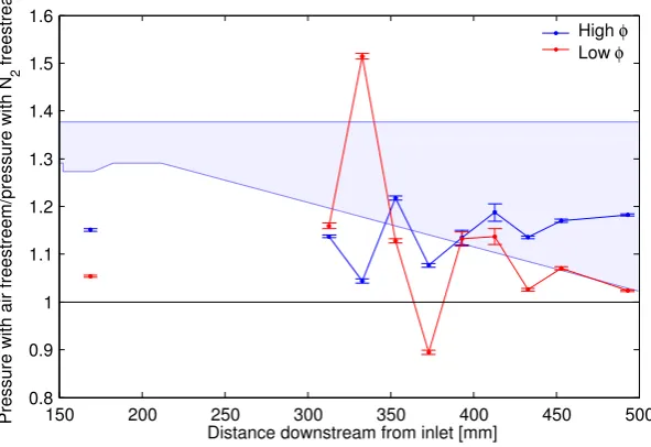
In order to determine the relative size of these two effects, hydrogen was in-jected into a nitrogen free-stream, inhibiting combustion, and this was com-pared to the same amount of hydrogen being injected into an air free-stream. The pressure difference between these two cases, then, is due only to the effect of combustion and is plotted in figure 8.2.

8.1. Confirmation of combustion 121

High φ

Low φ

150 200 250 300 350 400 450 500

0.8 0.9 1 1.1 1.2 1.3 1.4 1.5 1.6

Distance downstream from inlet [mm]

Pressure with air freestreem/pressure with N

2

freestream

Figure 8.2: The ratio of wall pressure when injecting into an air free-stream, to wall pressure when injecting into a nitrogen free-stream. This indicates the pressure

rise due to combustion. Data is averaged between1.5and2.5 msand error bars are

calculated from the standard error in the mean. The profile of the scramjet duct is shown for reference.

Visualisation experiments were also carried out by others in the vicinity of the cavity. These experiments used OH–PLIF [103] and are described in detail by references [80, 111]. Briefly, the output from a pulsed laser is formed into a sheet which illuminates a plane of the flow for a period of nanoseconds. A camera detects the luminosity emitted as molecules, having been excited by the laser sheet, relax back to their ground state. The luminosity signal is dependent on the concentration of the excited species, which wasOHin this case, but also on several other parameters of the flow including temperature and pressure. Therefore, in the configuration discussed here,OH–PLIF provides an indication of the location and relative abundance ofOHin a plane of the flow, but does not provide quantitative species concentration.

The PLIF images provided by Stotz and O’Byrne were corrected for pulse-to-pulse variation in the total laser energy and the spatial variation in the laser sheet. Flow luminosity was not subtracted, so that the images include a contri-bution from the flow luminosity as well as the fluorescence signal.

PLIF images from a plane centred on one of the central fuel jets are shown in figures 8.3 and 8.4 for the high and low equivalence ratios, respectively. For hydrogen combustion,OHis an important species to visualise since it is present only as an intermediate species in the combustion reaction. The distribution of

OH, therefore, indicates the parts of the flow where combustion is occurring. Abundant fluorescence is visible in each of the images above and downstream of the cavity, and is limited downstream by the extent of the laser sheet. The high equivalence ratio shows more fluorescence, and therefore has a higherOH

concentration, and higher penetration of OH into the duct. The presence of

Figure 8.3: OH–PLIF for highφrun with laser sheet directly above one of the central fuel jets, from references [80, 111].

and thatH2Omeasured downstream is a result of combustion and not simply ambient water vapour.

8.2 The source of measurement uncertainty

As well as information about theOHpresence, PLIF images also provide infor-mation about the turbulence of the flow. In figure 8.3, the stream-wise spacing between consecutive maxima in the luminosity signal is_. 20 mm. Assuming that these structures are transported by the main flow at the free-stream veloc-ity of2760 ms−1 then the time between consecutive maxima passing a station-ary point is∼ 7µs. From figure 7.5 on page 105, the time taken to scan across an absorption line is10µswhile, at10 kHz, the time required to scan over both absorption features is100µs.

Assuming that the turbulence timescale at the TDLAS measurement location is similar to that near the cavity, the diode laser sensor would be unable to resolve the high frequency turbulent fluctuations in the flow. If the flow prop-erties change in the time between the laser scanning across line 1 and line 2, a measurement error can be introduced. In a flow with steady temperature, for example, if the water vapour concentration changes between the time that the two lines are scanned then the line ratio, R_ls, would depend on the changing water vapour concentration as well as the temperature. In the temperature and water vapour time-series presented earlier, this effect shows up as random variability in the measurement.

8.3. Water vapour mixture fraction 123

Figure 8.4: OH–PLIF for lowφ run with laser sheet directly above one of the

central fuel jets, from references [80, 111].

line, the flow properties can change considerably during this time. Some frac-tion of the uncertainty in the fitted absorbance, therefore, is due to turbulent variation in flow properties changing the absorbance of the flow.

Turbulence also affects the measurement away from spectral lines. Upschulte, Miller and Allen [118, 119] found that beam steering determined their signal-to-noise ratio when measuring water vapour in a scramjet combustor. Beam steering changes the fraction of the probe beam that arrives on the active sur-face of the detector and its effect can be reduced by using a de-focused lens [72] in front of the detector or by using a larger detector and large aperture. Re-ducing sensitivity to beam-steering, however, increases the relative amount of luminosity that is captured by the detector.

In the present sensor, an interference filter was used to reject broadband lumi-nosity. This filter caused a sinusoid-like ripple in absorption which changed in phase from scan to scan. In bench-top experiments, a very small change in inci-dent beam angle resulted in a large change in the phase of the ripple. Therefore, it is believed that the change in beam angle due to beam steering is sufficient to interact with the interference filter and produce undesirable changes in the shape of the absorption baseline. The interaction of turbulence, beam steering and the interference filter are believed to be major contributors to the measure-ment uncertainty.

8.3 Water vapour mixture fraction

−0.5 0 0.5 1 1.5 2 2.5 3 3.5 4 0

5 10 15 20 25 30 35

Time since arrival of test gas [ms]

Pressure [kPa]

H₂ injection into air, high φ

H₂ injection into air, low φ

No injection, N₂

Figure 8.5: Pressure at duct wall, taken from three pressure-instrumented shock tunnel runs. The pressure transducer is mounted on the duct floor, near the probe

beam location and is smoothed with a20point running mean filter.

check on the TDLAS results is to use the measured temperature and number density to estimate the water vapour mixture fraction.

If we assume that the pressure of the components can be represented by Dal-ton’s law, then the partial pressure of water vapour is given by

PH2O =

NH2ORT NA10−6

(8.1)

where NH2O is the number density of water vapour

molecules cm−3, R =

8.314 Jmol−1K−1is the molar gas constant, Tis temperature [K],NA =6.022× 1023mol−1is Avogadro’s number and the factor of 10−6is present sinceNH2O is

expressed inmolecules cm−3_.

Close to the combustor wall, we assume that the local pressure is well approx-imated by the wall pressure. This is shown for the two equivalence ratios, and for no injection, in figure 8.5. At this location, there is a periodic modulation about a steady decay which is present in only some of the upstream traces. Neely et al. [75] noted similar features in their pressure measurements and attributed this to shock reflection off the wall in the vicinity of the pressure transducer. Slight variation in the position of the shock over the course of the shock tunnel test time would result in varying pressure as observed in figure 8.5.

By normalising water vapour partial pressure by the wall pressure, we obtain an approximation to the water vapour mixing ratio. This is the fraction of wa-ter molecules in the gas mixture, and is shown in figure 8.6. Figure 8.6 was calculated from the same data as was used to demonstrate repeatability in the previous chapter, which were from10.6 mmabove the scramjet floor.

Al-8.3. Water vapour mixture fraction 125

1 1.5 2 2.5 3 3.5 4

0 0.02 0.04 0.06 0.08 0.1 0.12 0.14 0.16 0.18 0.2

Time after shock reflection [ms] H2

O partial pressure normalised by wall pressure

high φ

low φ

Figure 8.6: Water partial pressure normalised by wall pressure, which is equiva-lent to the mole fraction of water if local pressure is the same as the wall pressure.

Calculated from the same data as figures 7.13 and 7.1410.6 mmfrom the duct floor.

though the global equivalence ratio is below1in each of the cases, some parts of the duct would have a local equivalence ratio of1 and therefore, if combus-tion is complete, it is feasible for parts of the duct to reach 35%water vapour. Measurements that indicate more than this, however, are physically impossible and would indicate an error in the measurement.

Shown in figure 8.6, after 1.5 ms the water vapour ratio is well below the the-oretical maximum of 35% in both the high and low equivalence ratio cases, although the larger scatter before1.5 mstakes some measurements above this. Having been determined for two fluctuating data sets, the inferred water frac-tion is highly variable but appears close to 0.08 at 2 ms for both equivalence ratios. Apart from the variability in the measurement, which declines over the test time, the water fraction appears relatively constant until3 mswhen it starts to decline rapidly in the low equivalence ratio case.

8.4 Comparison with CFD

Comparing TDLAS and CFD results is useful for two reasons:

• CFD provides full details of the flow-field within the scramjet and the 3–D CFD results can be used to find out how the assumption of homogeneous line-of-sight properties affects a simulated TDLAS measurement in the CFD flow; and

• Experimental results can be used to verify the accuracy of the CFD simu-lation.

Both of these aspects are considered in this section, although the comparison is limited by the apparant poor correspondence between the CFD result and conditions in the scramjet duct.

Before experiments were conducted, GASP version 3.2 [1] was used to compute the 3–D, chemically-reacting flow within the scramjet combustor. Attempts to obtain a turbulent solution were unsuccessful, however a solution was obtained using a laminar solver and this was used as an approximate guide to the possi-ble flow-field in the combustor during sensor design.

The laminar CFD results performed by the author were superseded by the ones presented here which were computed by Stotz using CFD++ version 4.2 [67]. Apart from the geometry changing downstream of the cavity from a straight to diverging duct, the computational model was identical to that described in references [80, 111].

Taking advantage of the symmetry of the combustor, the 3–D flow solution was computed for half of the duct using a Reynolds–averaged Navier–Stokes solver, using wall functions and a three-equation turbulence model (thek––Rmodel [44]). The combustor geometry was modelled with a rectangular mesh of 2.3

million cells. The cells were clustered in the cavity, particularly around the in-jector ports, and at the duct walls. The boundary layer of the duct was resolved in the model and contained around 15 cells near the TDLAS probe location. Cells were not tightly clustered in the vertical direction at the TDLAS beam lo-cation, however grid spacing was still much finer than the separation between individual probe beam locations.

Flow chemistry was simulated with the model by Drummondet al. [29] which includes 9 species and 18 reactions and treats nitrogen as inert. Since dissocia-tion of nitrogen and formadissocia-tion ofNOx was not allowed by this chemistry model, the flow entering the scramjet was modelled as a20%O2, 80%N2mixture. This is a simplification of the actual flow delivered by the facility which contains chemically frozen radicals generated in the stagnation region.

Other conditions at the CFD-model inlet were: pressure91.1 kPa, temperature

8.4. Comparison with CFD 127

0 50 100 150 200 250 300 350 400 450 500 0

50 100 150 200 250

Distance downstream from inlet [mm]

Pre

ss

ur

e

[k

P

a]

H₂ H2

No injection, N₂freestream

Figure 8.7: Measured and CFD-predicted pressure on the combustor floor.

Mea-sured pressure at each station is the mean pressure from1.25 msto1.75 ms,

nom-inally the pressure at1.5 ms, and error bars indicate the standard deviation over

this time. Note that the cavity transducer is10 mmfrom the centre-line. CFD by

Stotz.

injected at 5.65 gs−1 _{at a temperature of250 K. This is half of the flow rate of} experiments since the computational model included only half of the combus-tor.†

The pressure along the duct centre-line, as predicted by the CFD model, is slightly lower than the measured pressure at the ‘inlet’ transducer and in the cavity, as shown by figure 8.7. The standard deviation of pressure fluctuations at each measurement location is shown, indicating the large fluctuations in the cavity as well as the measurement noise associated with the inlet transducer. The inlet measurement also shows poor shot-to-shot repeatability which is not matched by the measurements further down the duct. Since the cavity trans-ducer was off-centre, the comparison between centre-line pressure is slightly misleading. According to the CFD prediction, pressure at the transducer loca-tion is10% lower than along the center-line. When this is taken into account, the CFD under-predicts the cavity pressure by a similar amount to the inlet pressure.

Pressure measurements beyond the cavity have mixed agreement. The first few upstream and furthest downstream measurements match CFD. However, the shape of the pressure distribution is not particularly well predicted by CFD. The CFD indicates a steadily decreasing pressure towards the end of the duct whereas measurements show the pressure to be almost constant in this region. Despite the noted differences however, the overall agreement between measure-ments and simulation is relatively good.

†_{Note also that the freestream conditions used for the CFD underestimated the temperature}

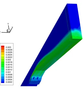
Figure 8.8: Temperature predicted by CFD, nominally matching the experimental conditions at the high equivalence ratio. The left of the image is the symmetry plane of the scramjet combustor and the scramjet exit is facing out of the page. The exit plane shows two cool spots, with the lower one being associated with high hydrogen concentration, as well as a hot layer attached to the wall. The green slice indicates the TDLAS measurement plane. CFD by Stotz.

Temperature predicted by the model is shown in figure 8.8. The wall tempera-ture is constant at300 Kto match the experimental scramjet, which has insuffi-cient time to heat significantly over the3 mstest. Along the scramjet centreline, the left of the model in figure 8.8, the shock structure is visible in the vicinity of the cavity. The flow then cools as it encounters the expansion fan after passing the diverging corner in the duct floor. The lower part of the duct contains a cool stream of gas which is mostly unburnt hydrogen. A second cool pocket is visible near the top of the duct, cooler due to the expanding flow, while a hot layer adheres to the wall of the duct at the right of the image.

The mole fraction for water vapour predicted by the model is shown in figure 8.9. This shows less structure than the temperature plot with water vapour visible only in the lower part of the duct. Although not visible at this scale, the model predicts water vapour all the way up the duct. Near the top of the duct, water vapour is mostly confined to the boundary layer.

8.4. Comparison with CFD 129

Figure 8.9: Water mole fraction predicted by CFD. CFD by Stotz.

Figure 8.10 shows temperature and water concentration in the measurement plane, overlaid with the probe beam locations. The traverse takes the beam through the cool pocket of gas near the duct floor and passes through the hot layer near the duct wall at each location.

As the beam moves up the duct, it passes through regions with decreasing water vapour concentration so that the topmost location passes through a region with comparatively little water. While temperature varies considerably along each line-of-sight, water concentration is relatively constant.

The data in figure 8.10 can be used to simulate a TDLAS measurement. Tem-perature and water concentration provide the information necessary to predict absorbance from each of the spectral lines, as described in section 4.2. The absorbance from a measurement can then be calculated by integrating this ab-sorbance along each of the beam paths and the analysis procedure used for the experimental data can be applied to this simulated experiment.

Horizontal mean compared with simulated TDLAS temperature and water con-centration are shown in figures 8.11 and 8.12 respectively. Near the bottom of the duct, measured temperature is low compared with the mean temperature because of the stronger absorption of line 1 at low temperature. Further up the duct, temperature is reported higher than the horizontal mean since the water vapour is located only in the hot boundary layer.

−20 0 20 0 10 20 30 40 50 60 70 80 90

Distance from duct centreline [mm]

Distance from duct floor [mm]

H 2

O concentration [molecules cm

−3 ] 0 0.5 1 1.5 2 2.5 3 3.5 4 x 1015

Temperature [K] 400 600 800 1000 1200 1400

Figure 8.10: Temperature (left) and water vapour (right) in the measurement plane, predicted by CFD for the high equivalence ratio case. Horizontal lines indi-cate the probe beam locations. CFD by Stotz.

0 10 20 30 40 50 60 70 80 90 100

200 400 600 800 1000 1200 1400 1600 1800 2000

Distance from duct floor [mm]

Te mper at ur e [K ]

Mean across duct

Result from simulated TDLAS Measurement at 1.5 ms

Figure 8.11: CFD-predicted line-of-sight mean temperature, apparent tempera-ture from TDLAS simulated from CFD data and measured temperatempera-ture. Plotted

measurements indicate the average and standard deviation from 1 to 2 ms and

8.4. Comparison with CFD 131

0 10 20 30 40 50 60 70 80 90 100

0 0.5 1 1.5 2 2.5 3 3.5

4x 10

15

Distance from duct floor [mm]

H 2

O concentration [molecules cm

−3 ]

Mean across duct

Result from simulated TDLAS

Figure 8.12: CFD-predicted line-of-sight mean and simulated TDLASH2O

concen-tration. Experimental results are shown in figure 7.16. CFD by Stotz.

measured with simulated TDLAS and the mean concentration across the duct. Water concentration is highest near the duct floor and decreases with increas-ing distance up the duct.

For both temperature and water vapour concentration, this suggests that the error with assuming a homogeneous beam path is relatively small provided that the CFD is producing a representative line-of-sight variation in flow properties. A limitation of this analysis is that the result produced by CFD represents a time-averaged solution to the turbulent flow-field. As such, the line-of-sight variability in flow properties is underestimated somewhat compared with the instantaneous variability in flow properties. This conclusion should also be tempered by the knowledge that the CFD massively underpredicts the water vapour concentration, as discussed next.

Besides providing an indication of how line-of-sight variability affects the mea-surement, the usefulness of the temperature and water vapour measurements can be illustrated by direct comparison with the CFD results.

As well as the simulated TDLAS results, experimental results are shown in figure 8.11. These are from the same data as the results presented in the pre-vious chapter, with the difference that data extracted from the time-series was centred on1.5 msinstead of2 msto match the CFD boundary conditions.

Diode laser measurements had large fluctuations early in the experimental run, so that the variability indicated in figure 8.11 is larger than that reported in the previous chapter. As before, the error bars indicate the standard deviation of the variability of the measurements rather than the error in the mean. Shot-to-shot variability is indicated by the repeated measurements at10.6 mm.

results differ from the measurements. Turbulent line-of-sight variability does not help explain this discrepancy either, since increasing the variability along the line of sight tends to decrease the measured temperature, suggesting that CFD is indeed predicting a low temperature.

The gulf between measurements and CFD predictions is considerably larger for water vapour concentration. Measured water concentration is not plotted in figure 8.12 since it is approximately102larger than the concentration predicted by CFD—TDLAS results were shown in figure 7.16. The extent of the water vapour is similar, with measured water vapour dropping to25%of it’s maximum at 40 mm from the duct floor, whereas CFD predictions put this point nearer

30 mm. The distribution shape is also similar. Although the measurements suggest that a peak in water concentration may be present at some distance from the wall, a monotonic decrease in concentration is within experimental uncertainty.

The main purpose of presenting these CFD results here is to illustrate the util-ity of TDLAS in verifying the results from a simulation. The CFD result is taken to be at fault here since PLIF results, presented earlier in this chapter, show strong combustion within the duct. This is inconsistent with water vapour concentrations of0.15%or less.

Nevertheless, it is worth considering some possible reasons why the discrep-ancy is so large, with a view to making improvements to the CFD simulation in the future.

Comparison with experiments saw that the simulation was under-predicting both water concentration and temperature. Since heat is released with the formation of water vapour, an increase in water production should result in an increase in temperature, and take both quantities towards better agreement.

In order for more hydrogen to react in the duct, it must first mix with oxygen from the free-stream. Although not shown, examination of the hydrogen mole fraction indicated that this mixing is indeed occurring—enough so that it is unlikely to be the limiting step.

Assuming that the mixing is modelled reasonably, the chosen chemistry model seems a likely candidate for further investigation. As noted above, the chem-istry model is comparatively simple and treats nitrogen as inert. In experi-ments, the free-stream contains a fraction of radicals and nitrogen compounds. These are formed in the stagnation region of the shock tunnel and have insuffi-cient time to recombine before encountering the scramjet flow. In some reaction models, the presence of small amounts of radicals has the ability to significantly decrease the ignition delay time [81]. If this were to happen, heat released be-fore the expansion might be sufficient to maintain a high enough temperature for combustion to continue after the expansion. In this way, a threshold could be reached where a small change could result in a disproportionate increase in water vapour concentration.†

In a simulation of a scramjet combustor, however, we encounter a supersonic, turbulent, chemically-reacting flow so there is ample opportunity for problems

†_{It is also likely that the CFD would agree better with observations if a hotter, and more}

8.4. Comparison with CFD 133