Parity and generalised Büchi automata

(1)

Determinisation and Complementation

Thesis submitted in accordance with the requirements of the University of Liverpool for the degree of

Doctor in Philosophy by

Praveen Thomas Methrayil Varghese

November 2014

(2)

Thesis committee: Prof. Dr. Wolfgang Thomas and Dr. Dominik Wojtczak

Supervisory team: Dr. Sven Schewe (Primary) and Prof. Dr. Frank Wolter (Sec-ondary)

(3)

Abstract

In this thesis, we study the problems of determinisation and complementation of finite automata on infinite words. We focus on two classes of automata that occur naturally: generalised Büchi automata and nondeterministic parity automata. Gen-eralised Büchi and parity automata occur naturally in model-checking, realisability checking and synthesis procedures. We first review a tight determinisation procedure for Büchi automata, which uses a simplification of Safra trees calledhistory trees. As Büchi automata are special types of both generalised Büchi and parity automata, we adjust the data structure to arrive at suitably tight determinisation constructions for both generalised Büchi and parity automata.

As the parity condition describes combinations of Büchi and CoBüchi conditions, instead of immediately modifying the data structure to handle parity automata,we arrive at a suitable data structure by first looking at a special case, Rabin automata with one accepting pair. One pair Rabin automata correspond to parity automata with three priorities and serve as a starting point to modify the structures that result from Büchi determinisation: we then nest these structures to reflect the standard parity condition and describe a direct determinisation construction.

The generalised Büchi condition is characterised by an accepting family with k

accepting sets. It is easy to extend classic determinisation constructions to handle generalised Büchi automata by incorporating the degeneralization algorithm in the determinisation construction. We extend the tight Büchi construction to do exactly this.

Our determinisation constructions go to deterministic Rabin automata. It is known that one can determinise to the more convenient parity condition by incor-porating the standardLatest Appearance Recordconstruction in the determinisation procedure. We determinise to parity automata using this technique.

We prove lower bounds on these constructions. In the case of determinisation to Rabin automata, our constructions are tight to the state. In the case of determini-sation to parity, there is a constant factor≤ 1.5 between upper and lower bounds reducing to optimal(to the state) in the case of Büchi and 1-pair Rabin.

(4)

(5)

Acknowledgements

I would like to express my deepest gratitude to my supervisor, Sven Schewe. I started my research based on his work about determinising Büchi automata and I am amazed that this particular problem evolved into the papers we published and finally became the backbone of this thesis. I owe my progress as a researcher to his supervision. I am also thankful to him for his friendship, pleasant company and the coffee breaks that brightened up the great British weather and that led to my coffee addiction.

My introduction to this line of research was Wolfgang Thomas’ excellent survey on ‘Languages, Automata, and Logic’. It is my great privilege to have had such a distinguished scientist as Wolfgang on my thesis examination committee along with Dominik Wojtczak. Their examination of my thesis gave me more perspective on my research and I thank them for their helpful comments which have improved my thesis greatly.

It was good fun to work with Ashutosh Trivedi on strategy improvement. I learnt a lot about a topic I had not worked on before and this work with Ashu and Sven led to a paper at ICALP. I am especially grateful for his great company on several evenings out in Liverpool.

I want to thank my colleagues in Liverpool – Petar Iliev, John Fearnley, Amir Kermani, Anshul Gupta, Ana Ozaki, Will Gatens, Julio Lemos and André Hernich. Thank you for all the inspiring, and even the random discussions over coffee, for the reading group and for making my time as a Ph.D. student more pleasurable.

Nir Piterman got me started withω-automata when I was a Master’s student at Leicester. I would not have been a researcher were it not for his supervision of my Master’s thesis and for this I am eternally indebted.

I wish to thank the EPSRC and the Department of Computer Science for support-ing my Ph.D. studies financially, especially the Department of Computer Science for providing a good research environment.

My time in Liverpool would have been a lot less enjoyable had I not met Gary, Hannah, Olivia and Nahum. Thank you Worralls for providing a place for me to stay, for feeding me, and for all the good times.

(6)

(7)

Declaration

I declare that this thesis was composed by myself, that the work contained herein is my own except where explicitly stated otherwise, that this work was undertaken during my period of study at the University of Liverpool and has not been submitted for any other degree or professional qualification except as specified.

The first section of chapter 3 contains a construction from [Sch09b]. This con-struction is modified to suit transition-labeled automata as input but the technical details are almost the same.

(8)

(9)

Chapter

1

Introduction

Finite automata on infinite structures and finite games of infinite duration are two

theories that have often influenced each other, both having been inspired by Church’s

realisability problem [Chu62]. The term "ω-automata" generally refers to finite au-tomata that accept or reject words of infinite length, or,ω-words. ω-automata were first introduced in Büchi’s decidability proof for the monadic second-order logic of

one successor (S1S) [Büc62]. Following from Büchi’s result, they have formed the

basis for the theories of model checking, realisability checking, and synthesis

proce-dures for linear time temporal logic (LTL) [Pnu77].

Theω-automata introduced by Büchi (that were subsequently named after him) extend the well known theory of finite automata on finite words to languages over

infinite words. Büchi automata are the most studied form of ω-automata. They extend finite automata in the sense that, while finite runs of finite automata are

accepting if an accepting state is visited at the end of the run, an infinite run of a

Büchi automaton is accepting if a final state is visited (or a final transition is taken)

infinitely many times during the course of the run. The Büchi acceptance condition

thus specifies a set of states(or transitions) that have to be visited(respectively, taken)

infinitely often.

Although the connection to finite automata on finite words might seem to

(14)

un-fortunately not the case. In particular, Büchi automata are not closed under

de-terminisation. While finite automata can simply be determinised with the subset

construction [RS59], it turns out that deterministic Büchi automata do not recognise

the same languages as nondeterministic Büchi automata. For example, deterministic

Büchi automata cannot recognise the simpleω-regular language that consists of all infinite words that contain only finitely many0’s over an alphabet{0,1}.

As a consequence of McNaughton’s result, there arose a need for more

spe-cific acceptance conditions, such as Muller’s subset condition, Rabin’s pairs

condi-tion [Rab69] or its dual, the Streett condicondi-tion [Str82], or theparity condition. Yan

established annΩ(n)lower bound for the determinisation of Büchi automata [Yan08] even for determinising to Muller automata, which implies that the standard subset,

or a breakpoint construction is not enough.

A related acceptance condition to the Büchi condition is the generalised Büchi

condition, which comprises of an accepting family. It requires that a final state (or

final transition) from each accepting set is visited (respectively, is taken) infinitely

many times. The standard translation from LTL to ω-automata [GPVW95] goes to generalised Büchi automata with the acceptance condition on the transitions.

In this thesis, we study the problems of the determinisation and complementation

of nondeterministic Büchi, generalised Büchi, and parity automata. We have already

outlined the importance of Büchi automata in the context of verification. The

stan-dard translation from LTL to automata results in generalised Büchi automata. Parity

automata are also particularly important, given that the parity condition naturally

recognizes languages specified by fixed-point expressions. Although

nondeterminis-tic parity automata are as equally expressive as Büchi automata, as they are more

succinct, they can easily encode other conditions, such as the intersection of Büchi

and co-Büchi conditions.

We studytransition-labeled automata in this thesis. Transition-based acceptance

mechanisms have proven to be a more natural target of automata transformations.

(15)

transition-based acceptance is straight forward, and the Safra-style determinisation

procedures from the literature [Saf88, Saf92, Pit07, Sch09b] have a natural

represen-tation with an acceptance condition on transitions. Their translation to state-based

acceptance is by multiplying the acceptance from the last transition to the statespace.

A similar observation can be made for other automata transformations, like the

removal ofε-transitions from translations ofµ-calculi [Wil01, SF06a] and the treat-ment of asynchronous systems [SF06b], where the state-space grows by

multipli-cation with the acceptance information (e.g., maximal priority on a finite sequence

of transitions), while it cannot grow in case of transition-based acceptance.

Sim-ilarly, tools like SPOT [Dur14] offer more concise automata with transition-based

acceptance mechanism as a translation from LTL. Using state-based acceptance in

the automaton that we want to determinise or complement would also complicate

the presentation of the complementation procedure. But first and foremost, using

transition-based acceptance provides cleaner results.

This is the case because in state-based acceptance, the role of the states is

over-loaded. In finite automata over infinite structures, each state represents the class of

tails of the word that can be accepted from this state. In state-based acceptance, they

have to account for the acceptance mechanism itself, too, while they are relieved

from this burden in transition-based acceptance. In complementation techniques

based on rankings, this results in a situation where states with certain properties,

such as final states for Büchi automata, can only occur with some ranks, but not with

all.

As transition-based acceptance separates these concerns, the presentation

be-comes cleaner. The natural downside is that, for example, we lose thenO(n) bound [CZ11b] for parity complementation, as the number of priorities in a parity

automa-ton with transition-based acceptance can grow arbitrarily. But in return, we do get a

(16)

1.1 Determinisation of

ω

-automata

The determinisation of ω-automata was a key step in Rabin’s extension of Büchi’s proof to the case of trees [Rab69]. Rabin’s proof built on McNaughton’s

dou-bly exponential determinisation construction [McN66]. Safra was the first to

in-troduce singly-exponential determinisation constructions for Büchi [Saf88] and

Streett [Saf92] automata and current determinisation techniques [Pit07, Sch09b]

build on Safra’s work. For instance, Schewe’s determinisation technique for Büchi

automata yielding deterministic Rabin automata[Sch09b] builds on Safra’s [Saf88]

and Piterman’s [Pit07] determinisation procedures. It uses a separation of concern,

where the main acceptance mechanism, represented by history trees, is separated

from the formal acceptance condition, e.g., a Rabin (used by [Saf88, Saf92]) or

par-ity condition (used by [Pit07]). History trees can be seen as a simplification of Safra

trees [Saf88]. In a nutshell, they represent a family of breakpoint constructions:

sufficiently many to identify an accepting run, and sufficiently few to be concise.

There are also other constructions that tackle determinisation from a different

viewpoint. An example is Muller and Schupp’s [MS95] presentation of a

nondeter-minisation technique for alternating tree automata shows a connection to the

de-terminisation of finite automata on infinite words. Kähler and Wilke build on this

construction in [KW08]. Although they start from a different viewpoint, their method

seems to converge with the Safra-based constructions.

In this thesis, we adapt Schewe’s determinisation procedure [Sch09b] to

deter-minise parity automata. We investigate what is required to handle such an

adap-tation and devise a similar determinisation procedure for nondeterministic parity

automata.

We also consider generalised Büchi automata. There are several ways to

deter-minise a generalised Büchi automaton withnstates andkaccepting sets. One could start with translating the resulting generalised Büchi automaton first to an ordinary

(17)

result-ing in a determinisation complexity of roughly(nk)O(nk)states, or one could treat it as a Streett automaton, which is equally expensive and has a more complex

deter-minisation construction.

Schewe’s determinisation procedure [Sch09b] again proves to be an easy target

for generalisation, because it separates the representation of the history of a run

from the acceptance condition. To extend this technique from ordinary to

gener-alised Büchi, it suffices to apply a round-robin approach to all breakpoints under

consideration. That is, each subset is enriched by a natural number identifying the

accepting set, for which we currently seek to see the following breakpoint. Each time

a breakpoint is reached, we turn to the next accepting set. Note that this algorithm

is a generalisation in the narrower sense: in case that there is exactly one

accept-ing set, it behaves exactly as the determinisation procedure for Büchi automata in

[Sch09b]. An algorithm to determinise generalised Büchi automata to deterministic

parity automata using this method was used in [KPV06], similarly extending

Piter-man’s construction [Pit07, LW09].

The constructions in this thesis provide Rabin automata as output. We give

es-timations of the size of the deterministic automata. In the case of nondeterministic

generalised Büchi automata, we find that for an automaton withnstates and k ac-cepting sets, we get a deterministic Rabin automaton withght_k(n)states and2n−1 Rabin pairs. The functionght_k(n)(enumerating the number of possible states of the deterministic automaton) is approximately(1.65n)n fork = 1, (3.13n)n for k = 2, and(4.62n)n fork = 3, and converges against(1.47kn)nfor large k. These bounds can also be used to establish smaller maximal sizes of minimal models, which is

useful for Safraless determinisation procedures [KV05, FS13, KPV06]. For the

trans-formation to deterministic parity automata from [Sch09b], we obtain an automaton

withO(n!2kn)states and2n+ 1priorities.

In the case of nondeterministic parity automata, we do not provide a similar

(18)

Büchi and 1-pair Rabin automata), but we show tightness up to a constant factor of

1.5.

Our constructions lead to deterministic Rabin automata as targets. While these

constructions are tight with respect to the number of states of the deterministic

automaton, the acceptance condition is exponential in the number of Rabin pairs.

Determinising to parity automata seems to be an even more attractive target since

emptiness games for parity automata [Sch07, JPZ08] have a lower computational

complexity compared to emptiness games for Streett or Rabin automata [PP06]. We

therefore show how we can obtain deterministic parity automata in each case by

using our construction to deterministic Rabin automata as an intermediate step.

Colcombet and Zdanowski [CZ09] showed that Schewe’s determinisation

pro-cedure for Büchi automata is optimal. We extend this lower bound to generalised

Büchi automata and parity automata generalising their techniques, showing that the

determinisation procedures are optimal.

1.1.1 Timeline of complexity results

We give here a timeline of the sequence of results with respect to the determinisation

problem for Büchi automata.

Target automaton Complexity

1966 - McNaughton Deterministic Muller 22O(n)

1988 - Safra Deterministic Rabin nO(n),≈12nn2n

2006 - Piterman Deterministic parity ≈n!nn

2009 - Liu and Wang, separately -Schewe Deterministic parity ≈n!2

2009 - Schewe Deterministic Rabin trace ≈(1.65n)n

2009 - Colcombet and Zdanowski Deterministic Rabin trace θ(1.65n)n

Table 1.1: Determinisation timeline for Büchi automata

In the case of Büchi determinisation, the best current determinisation

proce-dure that determinises to Rabin automata is Schewe’s construction [Sch09b]. A

tight matching bound for this construction is shown by Colcombet and Zdanowski in

(19)

as output is Piterman’s construction [Pit07]. We show in this thesis that the

con-struction in [Pit07] is optimal.

For generalised Büchi automata, a construction that is similar to Piterman’s Büchi

determinisation construction is shown in [KPV06]. This is the construction with the

best upper bound. We provide a matching lower bound for this construction. We also

provide matching upper and lower bounds for the determinisation of generalised

Büchi automata to deterministic Rabin automata.

There are two ways to determinise parity automata. One could convert them first

to Büchi automata and then apply one of the above constructions on them. The other

way is to directly determinise. We provide the first direct determinisation procedure

for parity automata along with tight bounds for the construction.

1.2 Complementation of

ω

-automata

The earliest results onω-automata involved the complementation problem. Büchi’s seminal paper [Büc62] on the correspondence between logic and automata showed

that Büchi automata are closed under complementation and introduced a

comple-mentation algorithm that uses Ramsey theory. Later results in the field of formal

veri-fication established the importance of the complementation problem forω-automata, for e.g., the language inclusion problem uses complementation [Kur94]. Another

important use of complementation is in checking the correctness of translation

tech-niques [Var07, TTH13a]. The GOAL tool [TTH13a] shows this with a test suite that

incorporates recent algorithms [Saf88, Tho99, KV01, Pit07] for Büchi

complementa-tion.

Given the importance of this problem, it is not surprising that the

complemen-tation ofω-automata is much researched. In particular, there has been a long and fruitful quest for the exact complexity of complementation algorithms for Büchi

(20)

FKV06, Pit07, Var07, Yan08]. We will highlight some of the important results with

respect to this problem now.

The first important result with respect to the complementation of ω−automata is Büchi’s proof that nondeterministic Büchi automata are closed under

complemen-tation. Using a Ramsey-based argument Büchi came up with a doubly-exponential

complementation algorithm [Büc62]. This is much harder than complementing

fi-nite automata on fifi-nite words — an exponential determinisation procedure followed

by a reversal of final states yields an efficient complementation algorithm that is

ex-ponential. The complexity of the determinisation problem forω-automata rules out an analogous algorithm with similar complexity.

Further results on the complexity of the complementation problem followed in

the late 1980s, starting with the discovery of an EXPTIME upper bound [Péc86,

PSVW87]. There was a caveat: the complementation techniques used produced

automata with up to2O(n2) states, meaning that there was still an exponential gap to the lower bounds of Sakoda and Sipser for the case of automata on finite words.

Safra’s brilliant algorithm for the determinisation of Büchi automata suggested

a nO(n) bound for Büchi complementation, an upper bound that was seemingly matched by Max Michel’s [Mic88]Ω(n!)lower bound implying that Büchi comple-mentation is innθ(n), suggesting that Safra’s determinisation procedure also resulted in tight complementation.

However, Vardi [Var07] rightly pointed out that this impression of tightness was

in fact not true, because the big-Oh notation in the exponent hides an nθ(n) gap between upper and lower bounds.

It turns out that complementation procedures forω-automata are more efficient than determinisation, contrary to the case of finite words. By studying alternating

automata, complementation procedures that bypassed determinisation were found.

The gap between upper ((6n)n) and lower bounds (from Michel) was then nar-rowed down to 2θ(n) _{by techniques that observe the run graphs of alternating}

(21)

A further refinement of the above complementation technique builds on "tight

level rankings" [FKV06, Yan08] improving the upper bound to O (0.96n)n. Yan [Yan08] usingfull automataimproved the lower bound for complementation to

Ω (0.76n)n

. Finally, Schewe [Sch09a] provided a matching upper bound, showing

tightness up to anO(n2)factor reducing to anO(n)factor for trace languages. For Rabin, Streett, and parity automata, there has been much progress [CZL09,

CZ11b, CZ11a], in particular establishing annθ(n) bound for parity complementa-tion with state-based acceptance, which has been a great improvement and pushed

tightness of parity complementation to the level known from Büchi complementation

since the late 80s [Saf88, Mic88].

In this thesis, we discuss a bridge between optimal determinisation and tight

complementation. We show how the nondeterministic power of an automaton can

be exploited by using a more concise data structure compared to determinisation (flat

trees instead of general ones). In the case of generalised Büchi automata, this bridge

again results in a generalisation of the Büchi complementation procedure discussed

in [Sch09a] in the narrower sense: for one accepting set, the resulting automata

coincide. We also provide a matching lower bound: we show for alphabetsLk_n that the size of a generalised Büchi automaton that recognises the complement of a full

generalised Büchi automaton withnstates andkaccepting sets must be larger than

|Lk

n|, while the ordinary Büchi automaton we construct is smaller than |Lkn+1+1|. For

largek– that is, ifkis not small compared ton–|Lk_n|is approximately kn e

n

. This

improves significantly over the Ω(nk)n

bound established by Yan [Yan08].

We then establish tight bounds for the complementation of parity automata with

transition-based acceptance. We get a clean and simple complementation procedure

based on a data structure we call flattened nested history trees (FNHTs), which is

inspired by a generalisation of history trees to multiple levels, one for each even

priority≥2. We show that any procedure that determinises full parity automata with

(22)

automaton that is to be complemented. Our complementation construction uses a

marker in addition for its acceptance mechanism. Essentially, it is used to mark some

position of interest in an FNHT. It accounts for theO(n)gap between the upper and lower bound. We show that, forπ≥2(and hence for Büchi automata upwards) the number of states of our complementation construction is bounded by 4n+ 1 times the lower bound.

1.2.1 Timeline of complexity results

We show here the timeline of results with respect to Büchi complementation.

Complexity

1966 - Büchi 22O(n)

1986 - Pecuchet 2O(n2)

1987 - Sistla, Vardi, Volper 2O(n2)

1988 - Safra nO(n)

1988 - Michel nΩ(n)

1991 - Klarlund O (6n)n

1997 - Kupferman, Vardi O (6n)n

2004 - Friedgut, Kupferman, Vardi o (1.06n)n

2006 - Yan ω (0.76n)n

2006 - Friedgut, Kupferman, Vardi o (0.97n)n

2009 - Schewe o (0.76n)n

Table 1.2: Timeline of complementation complexity results

In this thesis, we introduce direct complementation procedures for generalised

Büchi and parity automata and provide tight bounds.

1.3 Structure of thesis

InChapter 2, we define the necessary ideas needed for the problems of determinisa-tion and complementadeterminisa-tion. We describe different acceptance types of automata and

mention the folk results in this field.

In Chapter 3, we tackle the determinisation of several types of automata. We first review the tight Büchi construction. We then take a step towards the

(23)

automata with one accepting pair. We then expand the data structure required to

describe the state of the deterministic automaton for the case of parity

determinisa-tion and provide a construcdeterminisa-tion to directly determinise parity automata. Next, we

provide a construction to determinise generalised Büchi automata. All these

con-structions provide Rabin automata as output. We give estimations of the size of the

deterministic automata. We then show how we can determinise to deterministic

parity automata and we give estimations for these procedures.

InChapter 4, we prove lower bounds for our constructions.

In Chapter 5, we discuss a bridge between optimal determinisation and tight complementation and show tight bounds for our complementation procedures.

(24)

(25)

Chapter

2

Preliminaries & problem statements

2.1 Preliminaries

We denote the set of non-negative integers byω, i.e. ω ={0,1,2,3, ...}. For a finite alphabetΣ, an infiniteword α is an infinite sequenceα0α1α2· · · of letters fromΣ.

We sometimes interpretω-words as functionsα :i7→ αi, and useΣω to denote the

ω-words overΣ.

Automata on infinite words. ω-automata are finite automata that are interpreted over infinite words and recognise ω-regular languages L ⊆ Σω. Nondeterministic

ω-automata are quintuplesN = (Q,Σ, I, T,F), where,

• Qis a finite set of states,

• I is a non-empty subsetI ⊆Qof initial states,

• Σis a finite alphabet,

• T :Q×Σ×Qis a transition relation that maps states and input letters to sets of successor states and,

• Fis an acceptance component. In this thesis, we consider Rabin, Streett, parity,

(26)

Runs and transitions. Arunρ of a nondeterministicω-automatonN on an input wordαis an infinite sequenceρ:ω→Qof states ofN, also denotedρ=q0q1q2· · · ∈ Qω_{, such that the first symbol of} _ρ _{is an initial state} _q

0 ∈ I and, for all i ∈ ω, (qi, αi, qi+1)∈T is a validtransition.

For a runρon a wordα, we denote withρ:i7→ ρ(i), α(i), ρ(i+1)

the transitions

of ρ. Let infin(ρ) = {q ∈ Q | ∀i ∈ ω ∃j > isuch thatρ(j) = q} denote the set of all states that occur infinitely often during the runρ. Likewise, let infin(ρ) = {t ∈ T | ∀i∈ω ∃j > isuch thatρ(j) =t}denote the set of all transitions that are taken infinitely many times inρ.

For technical convenience we also allow for finite runsq0q1q2. . . qnwithT∩{qn}×

{α(n)} ×Q=∅. Naturally, no finite run satisfies anyω-acceptance condition. Finite runs are rejecting, and have no influence on the language of an automaton.

Acceptance conditions. In this thesis, we use acceptance conditions over transi-tions. Acceptance mechanisms over states can be defined accordingly. Rabin

au-tomata areω-automata, whose acceptance is referring to a family of pairs{(Ai, Ri)|

i ∈ J}, with Ai, Ri ⊆ T, of accepting and rejecting transitions for all indices i

of some index set J. A run ρ of a Rabin automaton is accepting if there is an in-dexi ∈ J, such that infinitely many accepting transitions t ∈ Ai, but only finitely

many rejecting transitions t ∈ Rj occur in ρ. That is, if there is an i ∈ J such that

infin(ρ)∩Ai 6=∅=infin(ρ)∩Ri.

ω-automata that use the complementary Streettcondition are called Streett au-tomata. Their acceptance is defined by a family of pairs {(Gi, Bi) | i ∈ J}, with

Gi, Bi ⊆T, of good and bad transitions for all indicesiof some index setJ. A run

ρ of a Streett automaton is acceptingif, for all indices i ∈ J, some good transition

t∈Gior no bad transitiont∈Bj occur infinitely often inρ. That is, if, for alli∈J,

infin(ρ)∩Gi6=∅orinfin(ρ)∩Bi =∅holds.

One-pair Rabin automata R₁ = Q,Σ, I, T,(A, R)

(27)

singleton index set, such that we directly refer to the only pair(A, R). They are of special technical interest in this paper.

Parity automata (first introduced by Mostowski in [Mos84]) are ω-automata,

whose acceptance is defined by a priority function pri : T → Π that maps transi-tions to a finite setΠ ⊂ ω of non-negative integers. A runρ of a parity automaton isacceptingiflim sup_n→∞pri ρ(n)

is even, that is, if the highest priority that occurs

infinitely often in the transitions ofρis even. Parity automata can be viewed as spe-cial Rabin, or as spespe-cial Streett automata. In older works, the parity condition was

referred to as Rabin chain condition—because one can represent them by choosing

Ai as the set of states with priority ≤ 2iandRi as the sets of states with priorities

≤2i−1, resulting in a chainAi ⊆Ri ⊆Ai+1 ⊆. . .—or a Streett chain condition—

whereGiis the set of states with priority≥2i, andBiis the set of states with priority

≥2i−1. Some works also refer to the parity condition as theMostowskicondition. Parity automata with Π ⊆ {1,2} are called Büchi automata. They can also be viewed as one-pair Rabin automata with an empty set of rejecting states R = ∅. Büchi automata are denotedB = (Q,Σ, I, T, F), whereF ⊆ T are called the final or accepting transitions. A run is accepting if it contains infinitely many accepting

transitions.Bis thus a rendering of the parity automaton, where pri:t7→2ift∈F

andpri:t7→1ift /∈F.

We assume without loss of generality that the set Π of priorities satisfies that

min Π ∈ {0,1}. If this is not the case, we can simply change pri accordingly to

pri0 :t7→pri(t)−2several times until this constraint is satisfied. We likewise assume that Π has no holes, that is, Π = {i ∈ ω | max Π ≥ i ≥ min Π}. If there is a hole

h /∈Πwithmax Π> h >min Π, we can changepritopri0 :t7→pri(t)ifpri(t)< hand

pri0 :t7→pri(t)−2ifpri(t)> h. Obviously, these changes do not affect the acceptance of any run, and applying finitely many of these changes bringsΠ into this normal

form.

The different priorities have a natural order <, where i j if i is even andj

(28)

of priorities, optΠ0 = {i ∈ Π0 | ∀j ∈ Π0. i < j} denotes the optimal priority for acceptance.

Finally we definegeneralised Büchiautomata that include the acceptance

compo-nent Fi, where Fi is a family of accepting (or final) sets. A run ρ of a generalised

Büchi automaton is accepting if it contains infinitely many transitions from all final

sets (∀i∈[k](wherekis the cardinality ofFi),inf(ρ)∩Fi6=∅).

For all types of automata, a wordα is accepted by an automatonAif, and only if, it has an accepting run, and its languageL(A)is the set of words it accepts.

Deterministic automata. We call an automaton(Q,Σ, I, T,F)deterministicifI is singleton and T contains at most one target node for all pairs of states and input letters, that is, if (q, α, r),(q, α, s) ∈ T implies r = s. Deterministic automata are denoted(Q,Σ, q0, δ,F), whereq0is the only initial state andδis the partial function

withδ : (q, α)7→r⇔(q, α, r)∈T.

As deterministic automata can block, we also allow them to accept immediately.

Technically, one can use a state>which every automaton has. From>, all transitions

go back to >, and sequences that contain one (and thus almost only) > states are

accepting. This state is not counted to the state-spaceQ. If we want to include it, we explicitly writeQ>.

Theorem 2.1.1 (McNaughton’s Theorem) LetΣ be an alphabet and L ⊆ Σω be a

Büchi recognisable language. ThenLis recognised by a deterministic Muller automaton

(and therefore by a deterministic Rabin or parity automaton). [McN66]

Determinisation. For ω-automata, determinisation is a consequence of Mc-Naughton’s theorem. Given a nondeterministic automatonArecognising a language

L(A), determinisation is a procedure performed on A that returns a deterministic

(29)

Complementation. Given a nondeterministic automatonArecognising a language

L(A), complementation is a procedure performed onAthat returns a an automaton

Crecognising the complementary languageL(A).

2.2 Current results for determinisation and

complementa-tion

Theorem 2.2.1 Given a nondeterministic Büchi automaton withnstates, we obtain a

deterministic Rabin automaton with2O(n log n)states andnRabin pairs. [Saf88]

The above result establishes asymptotic upper bounds for both determinisation and

complementation of Büchi automata.

deterministic parity automaton withO(n!2)states and a2nparity index. [Pit07]

deterministic Rabin automaton with approximately(1.65n)n states and 2n−1 Rabin

pairs. [Sch09b]

Theorem 2.2.4 The determinisation construction described in [Sch09b] that takes a

nondeterministic Büchi automaton withn states and returns a eterministic Rabin

au-tomaton with approximately(1.65n)nstates and2n−1Rabin pairs is tight with respect

to the number of states. [CZ09]

Theorem 2.2.5 The problem of complementing a Büchi automaton is inΩ((0.76n)n). [Yan08]

Theorem 2.2.6 Given a nondeterministic Büchi automaton withnstates, we construct

a Büchi automaton witho (0.76n)nstates that accepts the complement language. This

(30)

Note that the parameter n stands for the number of states in the above state-ments. Note also that we are primarily concerned with state complexity in this thesis.

Optimising for two parameters, i.e., states and transitions is another question that is

interesting from a technical standpoint.

2.3 Problem statements

In this thesis, we will study the following problems:

1. We are given a nondeterministic parity automaton P. Can we directly

deter-miniseP again to a parity automaton without first translating to

nondetermin-istic Büchi automata?

2. Can we prove tight lower bounds for this construction?

3. Can we devise a tight complementation construction to complementP?

4. Given a nondeterministic generalised Büchi automatonGB, can we devise

(31)

Chapter

3

Determinisation constructions

In this chapter, we study the problem of determinisation of parity automata and

gen-eralised Büchi automata. We first review the tight construction of Büchi automata

from [Sch09b]. We then take a step towards the determinisation of parity automata

by extending the Büchi determinisation algorithm to a slightly more succinct

accep-tance condition. We then generalise this algorithm to determinise parity automata.

In a different extension, we extend the Büchi determinisation algorithm to

deter-minise generalised Büchi automata. The results in Sections 3.2, 3.3, 3.4 and 3.5 are

published in [SV14a] and [SV12].

3.1 Determinising Büchi automata

In this section, we outline a variant ([Sch09b]) of Safra’s determinisation

construction[Saf88] for Büchi automata. This construction was proved to be tight

in [CZ09]. It is a variant of Safra’s construction in the sense that there is a slight

difference in the data structure used to describe the states of the deterministic

au-tomaton. The construction itself does not differ from Safra’s except with respect to

(32)

3.1.1 History trees

Omega automata can have infinitely many possible runs on a given word. Safra trees

introduced in [Saf88] are a succinct representation of the possible initial prefixes of

these runs of a Büchi automaton B on an input wordα. History trees, introduced in [Sch09b] are slightly modified Safra trees and achieve the same objectives. The

main difference between Safra trees and history trees is the omission of explicit node

names.

Definition 3.1.1 A history treeis an ordered labelled tree (T, l), where T is a finite,

prefix closed subset of finite sequences of natural numbersω. Every element v ∈ T is

called a node. Prefix closedness implies that, if a node v = n1. . . njnj+1 ∈ T is in

T, then v0 = n1. . . nj is also in T. We call v0 the predecessor of v, denotedpred(v).

The empty sequence∈ T is called theroot of the ordered treeT. Obviously,has no

predecessor.

We further require T to be order closed with respect to siblings: if a node v =

n1. . . nj is inT, thenv0 = n1. . . nj−1iis also inT for all i ∈ ω withi < nj. In this

case, we callv0anolder siblingofv(andvayounger siblingofv0). We denote the set

of older siblings ofvbyos(v).

A history tree is a tree labelled with sets of automata states. That is, l : T →

2Qr{∅}is a labelling function, which maps nodes ofT to non-empty sets of automata

states. For Büchi automata, the labelling is subject to the following criteria.

1. The label of each node is a subset of the label of its predecessor:

l(v)⊆l(pred(v))holds for allε6=v∈ T.

2. The intersection of the labels of two siblings is disjoint:

∀v, v0∈T. v6=v0∧pred(v)=pred(v0)⇒l(v)∩l(v0) =∅.

3. The union of the labels of all siblings isstrictly contained in the label of their

predecessor:

(33)

We denote the number of history trees for Büchi automata havingn states with

ht(n). An estimation for the number of history trees produced when determinising a Büchi automaton is given in Subsection 3.5.1.

3.1.2 Construction

Let B = (Q,Σ, I, T, F) be a nondeterministic Büchi automaton with |Q| = n

states. We will construct an equivalent deterministic Rabin automaton D =

(D,Σ, d0, δ,{(Ai, Ri)|i∈J})where,

• Dis the set of history trees overQ,

• d0 is the history tree({ε}, l:ε7→I),

• J is the set of nodes that occur in some ordered tree of sizen,

• for every treed∈ Dand letterσ ∈Σ, the transitiond0 = ∆(d, σ) is the result of the transition mechanism described below.

Transition mechanism

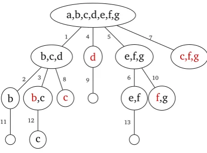
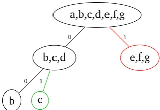
We will illustrate in parallel the transition mechanism using the example fragment

from Figure 3.1 on reading a letterσ. The starting history tree is shown in Figure 3.2.

We determine∆: (T, l), σ7→(T0, l0)as follows:

1. Update of node labels (subset constructions).

We update l to the functionl1 by assigning, for allv ∈ T, l1 : v 7→ {q ∈ Q | ∃q0 ∈l(v).(q0, σ, q)∈T}, i.e., to theσsuccessors ofl(v).

2. Splitting of run threads / spawning new children.

In this step, we spawn new children for every node in the history tree. For

all nodes, we spawn a child labelled with the set of states reached through

(34)

a e b

g f

[image:34.595.180.372.112.297.2]

d c

Figure 3.1: Transition graph for the example fragment of a Büchi automaton on reading the letterσ. Double arrows represent accepting transitions

a,b,c,d,e,f,g

b,e,f c d,g

e f g

0 1 2

[image:34.595.196.354.381.490.2]

0 1 0

Figure 3.2: Starting example history tree

a,b,c,d,e,f,g

b,c,d d e,f,g

b b,c e,f

0 1 2

0 1 0

[image:34.595.197.354.562.675.2]

(35)

a,b,c,d,e,f,g

b,c,d d e,f,g c,f,g

b b,c c e,f f,g

c

0 1 2 3

0 1 2 0 0 1

[image:35.595.214.427.99.254.2]

0 0 ₀

Figure 3.4: In Step 2, we spawn new children for every node in the history tree. A child node is labelled with it’s parent’s label minus the set of states that do not have an incoming accepting transition. If there is no state in the label of the parent that can be reached through an accepting transition, then the label of the child will be empty, eg. node 010. Although not part of this step, we show in red the states that are duplicated in younger siblings that are marked for removal in the next step

Thus, for every node ε ∈ d with c children, we spawn a new child vc and expand l1 tovcby assigning l1 : vc7→ {q ∈ Q | ∃q0 ∈l(v).(q0, σ, q) ∈ A}. We

useTnto denote the extended tree that includes the new children.

3. Removing states from labels – horizontal pruning.

We obtain a functionl2 froml1by removing, for every nodevwith labell(v) = Q0 and all statesq ∈Q0,qfrom the labels of all younger siblings ofvand all of their descendants.

4. Identifying breakpoints – vertical pruning.

We denote with T_e ⊆ T_n the set of all nodesv whose labell2(v) is now equal

to the union of the labels of its children. We obtainT_v fromT_nby removing all descendants of nodes inT_e, and restrict the domain ofl2accordingly.

During the run of an automaton, a point is reached from which accepting states

are visited again and again. We call such a point a breakpoint. Nodes inTv∩

Te represent the breakpoints reached during the infinite runρ and are called

(36)

a,b,c,d,e,f,g

b,c,d e,f,g

b c e,f g

c

0 ₁ 2 ₃

0 1 ₂ 0 0 1

[image:36.595.177.378.154.307.2]

0 0 0

Figure 3.5: In Step 3, we remove from the label of younger siblings and their descen-dants, those states that are already present in an older sibling.

a,b,c,d,e,f,g

b,c,d e,f,g

b c

0 ₁ 2 ₃

0 1 ₂ 0 ₀ ₁

0 0 0

[image:36.595.177.376.470.622.2]

(37)

a,b,c,d,e,f,g

b,c,d e,f,g

b c

0 2

[image:37.595.239.399.99.208.2]

0 1

Figure 3.7: In Step 5, we remove the empty nodes. The resulting tree may not be ordered.

5. Removing nodes with empty label.

We denote withT_r ={v∈ T_v |l2(v)6=∅}the subtree ofTv that consists of the

nodes with non-empty label and restrict the domain ofl2 accordingly.

6. Reordering.

To repair the orderedness, we call kvk = |os(v) ∩ Tr| the number of

(still existing) older siblings of v, and map v = n1. . . nj to v0 =

kn1k kn1n2k kn1n2n3k. . .kvk, denotedrename(v).

ForT0 ₌_rename₍_T

r), we update a pair(Tr, l2)from Step 5 tod0 = T0, l0

with

l0:rename(v)7→l2(v).

We call a node v ∈ T0∩ T stableifv = rename(v), and we call all nodes inJ

rejecting if they are not stable. That is, the transition will be in Rv exactly for

thosev∈J, such thatvis not a stable node inT ∩ T0.

3.1.3 Correctness

In order to establish the correctness of our determinisation construction, we need to

prove thatL(B) =L(D), that is, we need to ascertain that theω-language accepted by the nondeterministic Büchi automaton is equivalent to theω-language accepted by the deterministic Rabin automaton.

(38)

a,b,c,d,e,f,g

b,c,d e,f,g

b c

0 1

[image:38.595.196.355.99.208.2]

0 1

Figure 3.8: In Step 6, we reorder the tree and consider only those breakpoints that have not been reordered to characterise the current history tree in the Rabin accep-tance condition. For example, this history tree is added to the accepting set with index 001, A001. As the node 01 was reordered from 02, it is considered rejecting

and indicates that this tree will be added to the rejecting setR01.

α, there is a node v ∈ J that is stable infinitely often from some point in the run and

always accepting eventually during the run ofDonα.

Notation. For a stateq ofBand a history treed= (T, l), we call a nodevthehost node ofq, denotedhost(q, d), ifq ∈l(v), but not inl(vc)for any childvcofv.

Proof idea. The idea is that the state of each accepting run is eventually ‘trapped’ in

the same node of the history tree, and this node must be accepting infinitely often.

Letd0, d1. . .be the run ofDonαandq0, q1, . . .an accepting run ofBonα. Then we

can define a sequence v0, v1, . . . with vi = host(qi, di), and there must be a longest

eventually stable prefixvin this sequence.

An inductive argument can then be exploited to show that, once this prefixv is henceforth stable, the index v cannot be rejecting. The assumption that there is a point in time wherev is stable but never again accepting leads to a contradiction. Once the transition (qi, α(i), qi+1) is accepting, qi+1 ∈ li+1(vc) for some c ∈ ω and

for di+1 = (Ti+1, li+1). As v is never again accepting orrejecting, we can show for

all j > i that, if qj ∈ lj(vcj), then qj+1 ∈ lj+1(vcj+1) for some cj+1 ≤ cj. This

monotonicity leads to a contradiction with the assumption thatvis thelongeststable prefix.

(39)

letρD =d0d1. . .be the run of Donα. We then define the related sequence of host

nodesϑ=v0v1v2. . .=host(q0, d0)host(q1, d1)host(q2, d2). . ..

We defines= lim infn→∞|vn|to be the shortest length occurring infinitely often

of those host nodes. We follow this run and argue that the initial sequence of lengths

of the nodes inϑeventually stabilises. Leti0 < i1< i2 < . . .be an infinite ascending

chain of indices such that

1. (qj, α(j), qj+1)∈T is a transition for anyj≥i0,

2. the length|vj| ≥sof the j-th node is not smaller thansfor allj ≥i0, and

3. the length|vj|=sis equal tosfor all indicesj ∈ {i0, i1, i2, . . .}in this chain.

(1), (2) and (3) together imply that when we follow the run of the deterministic

automaton in positionsi0, i1, i2, . . ., the host nodesvi0, vi1, vi2, . . .form a descending

chain when the single nodesvi are compared by lexicographic order. As the domain

is finite, almost all elements of the descending chain are equal, say vi := π. In

particular,π ∈J is stable infinitely often from some point onwards.

We now assume for contradiction that this stable prefixπis accepting only finitely often. We choose an indexifrom the above defined ascending chaini0 < i1 < i2 < . . .such that

1. π is stable for allj≥iand

2. π is not accepting for anyj≥i.

Note thatπ is the host ofqi fordi, andqj ∈lj(π)holds for allj≥i.

Asρis accepting, there is a smallest indexj > isuch that(qj−1, α(j−1), qj)∈A.

Now, asπis stable but not accepting for allk≥i(and hence for allk≥j),qkmust

henceforth be in the label of a child ofπindk, which contradicts the assumption that

infinitely many nodes inϑhave lengths=|π|.

(40)

Lemma 3.1.3 [L(D) ⊆ L(B)] Given that there is a node v ∈ J, which is eventually

stable infinitely often and always accepting eventually for anω-wordα, then there is an

accepting run ofBonα.

Notation. For an ω-wordα andj ≥ i, we denote with α[i, j[the word α(i)α(i+ 1)α(i+ 2). . . α(j−1).

We denote withQ1 →α Q2 for a finite wordα =α1. . . αj−1 that there is, for all qj ∈ Q2 a sequence q1. . . qj withq1 ∈ Q1 and (qi, αi, qi+1) ∈ T for all1 ≤ i < j.

If, for allqj ∈Q2, there is such a sequence that contains a transition inF, we write Q1⇒αQ2.

Proof. Let α ∈ L(D). Then there is av that is eventually stable stable infinitely often from some point and always accepting eventually in the runρD ofDonα. We

pick such av.

Theproof ideais the usual way of building a tree of initial sequences of runs. Let

i0 < i1 < i2< . . .be an infinite ascending chain of indices such that

• vis stable for all transitions(dj−1, α(j−1), dj)withj≥i0, and

• the chaini0 < i1 < i2 < . . . contains exactly those indices i ≥ i0 such that (di−1, α(i−1), di)is accepting.

Letdi = (Ti, li)for alli∈ω. By construction, we have

• I →α[0,i0[_l

i0(v), and • lij(v)⇒

α[ij,ij+1[_l

ij+1(v).

Using this observation, we can build a tree of initial sequences of runs as follows:

we build a tree of initial sequences of runs ofBthat contains a sequenceq0q1q2. . . qij

for anyj∈ωif, and only if,

• (qi, α(i), qi+1)∈T is a transition ofBfor alli < ij, and

• for allk < jthere is ani∈[ik, ik+1[such that(qi, α(i), qi+1)∈Fis an accepting

(41)

By construction, this tree has the following properties:

• it is infinite,

• it is finitely branching,

• for allj ∈ω, a branch of length> ij contains at leastjaccepting transitions.

Exploiting König’s lemma, the first two properties provide us with an infinite

path, which is a run of B on α. The third property then implies that this run is

accepting. αis therefore in the language ofB. 2

The lemmata 3.1.2 and 3.1.3 together provide the following corollary.

Corollary 3.1.4 L(R) =L(D).

3.2 Towards the determinisation of parity automata

We will now start to extend the construction in the previous section to directly

de-terminise parity automata.

Since the parity condition is in fact, a nested condition, it makes sense to nest

history trees to handle the parity condition. However, the parity condition is a

nest-ing of Büchi and coBüchi conditions, and for this reason, we will need to nest trees

that handle the coBüchi condition in addition to the Büchi condition. The simplest

acceptance condition that is a combination of Büchi and coBüchi is the Rabin

con-dition with one pair. This also corresponds to a parity concon-dition with 3 colours. We

will describe how to modify history trees to handle this acceptance condition and

also show a determinisation construction for this acceptance condition.

3.2.1 Root history trees

(42)

Definition 3.2.1 (Root History Tree) Aroot history tree is a tree labelled with sets

of automata states. That is,l:T →2Qr{∅}is a labelling function, which maps nodes

ofT to non-empty sets of automata states.

For 1-pair Rabin automata, the labelling is subject to the following criteria.

1. The label of each node is a subset of the label of its predecessor:

l(v)⊆l(pred(v))holds for allε6=v∈ T.

2. The intersection of the labels of two siblings is disjoint:

3. The union of the labels of all siblings is contained, but not necessarily strictly

contained in the label of their predecessor:

∀v∈ Tr{ε} ∃q∈l(v)∀v0 ∈ T. v=pred(v0)⇒q /∈l(v0).

4. The label of the rootεequalsthe union of its children’s labels:

l(ε) =S

{l(v)|v∈ T ∩ω}.

Thus, aroot history tree(RHT) satisfies (1) and (2) from the definition of history

trees, and a relaxed version of (3) that allows for non-strict containment of the label

of the root.

Note that the 1-pair Rabin condition has an accepting and a rejecting

compo-nent. Our modification allows for a transition step where only the youngest child

of the root contains states which are reachable through rejecting transitions. All

other children will contain successors reachable only through accepting and neutral

transitions as in the Büchi construction.

3.2.2 Construction

LetR₁ = (Q,Σ, I, T,(A, R))be a nondeterministic one-pair Rabin automaton with

(43)

• Dis the set of RHTs overQ,

• d0 is the history tree({ε,0}, l:ε7→I, l: 07→I),

• J is the set of nodes 6= ε that occur in some RHT of size n+ 1 (due to the exemption for the root in Rule (4) in the definition of RHTs, an RHT can contain

at mostn+ 1nodes), and

• for every treed∈ Dand letterσ ∈Σ, the transitiond0 = ∆(d, σ) is the result of the sequence of the transition mechanism described below.

The index set is the set of nodes, and, for each index, the accepting and

reject-ing sets refer to this node.

Transition mechanism for determinising one-pair Rabin Automata

We determine∆: (T, l), σ7→(T0, l0)as follows:

1. Update of node labels (subset constructions).

The root of a history tree dcollects the momentarily reachable statesQr ⊆Q

of the automatonR₁. In the first step of the construction, we update the label

of the root to the set of reachable states upon reading a letter σ ∈ Σ, using the classical subset construction. We update the label of every other node

of the RHT dto reflect the successors reachable through accepting or neutral transitions.

For ε, we update l to the function l1 by assigning l1 : ε 7→ {q0 ∈ Q | ∃q ∈ l(ε).(q, σ, q0) ∈ T}, and for allε 6= v ∈ T, we update l to the functionl1 by

assigningl1 :v7→ {q0 ∈Q| ∃q∈l(v).(q, σ, q0)∈TrR}.

2. Splitting of run threads / spawning new children.

In this step, we spawn new children for every node in the RHT. For nodes

(44)

Thus, for every nodeε6=v ∈dwithcchildren, we spawn a new childvcand expandl1 to vcby assigningl1 :vc 7→ {q ∈ Q | ∃q0 ∈ l(v).(q0, σ, q) ∈ A}. If εhas cchildren, we spawn a new child c of the root εand expandl1 to cby

assigningl1 : c 7→ l1(ε). We use Tnto denote the extended tree that includes

the new children.

3. Removing states from labels – horizontal pruning.

We obtain a functionl2 froml1by removing, for every nodevwith labell(v) = Q0and all statesq∈Q0,qfrom the labels of all younger siblings ofvand all of their descendants.

4. Identifying breakpoints – vertical pruning.

We denote withTe⊆ Tnthe set of all nodesv=6 εwhose labell2(v)is now equal

to the union of the labels of its children. We obtainTv fromTnby removing all

descendants of nodes inTe, and restrict the domain ofl2 accordingly.

Nodes in T_v ∩ T_e represent the breakpoints reached during the infinite run ρ

and are called accepting, that is, the transition ofD₁ will be inAv for exactly

thev∈ Tv∩ Te. Note that the root cannot be accepting.

5. Removing nodes with empty label.

We denote withTr ={v∈ Tv |l2(v) 6=∅}the subtree ofTv that consists of the

nodes with non-empty label and restrict the domain ofl2 accordingly.

6. Reordering.

To repair the orderedness, we call kvk = |os(v) ∩ Tr| the number of

(still existing) older siblings of v, and map v = n1. . . nj to v0 =

kn1k kn1n2k kn1n2n3k. . .kvk, denotedrename(v).

ForT0 ₌_rename₍_T

r), we update a pair(Tr, l2)from Step 5 tod0 = T0, l0

with

l0 :rename(v)7→l2(v).

(45)

rejecting if they are not stable. That is, the transition will be in Rv exactly for

thosev∈J, such thatvis not a stable node inT ∩ T0.

Note that this construction is a generalisation of the same construction for Büchi

automata: ifR =∅, then the label of0is always the label ofεin this construction, and the node1is not part of any reachable RHT. (We would merely write0in front

of every node of a history tree.)

Correctness

The correctness proof of this construction follows the same lines as the correctness

proof of the Büchi construction.

Lemma 3.2.2 [L(R1) ⊆L(D1)] Given that there is an accepting run ofR1 on anω

-wordα, there is a node v ∈ J that is eventually always stable and always eventually

accepting in the run ofD₁onα.

Proof idea. Theproof ideaand notation are the same as for Büchi determinisation:

the state of each accepting run is eventually ‘trapped’ in the same node of the RHT,

and this node must be accepting infinitely often. Letd0, d1. . .be the run ofD1 onα

andq0, q1, . . .an accepting run ofR1 onα. Then we can define a sequencev0, v1, . . .

withvi = host(qi, di), and there must be a longest eventually stable prefix v in this

sequence.

An inductive argument can then be exploited to show that, once this prefixv is henceforth stable, the index v cannot be rejecting. The assumption that there is a point in time wherevis stable but never again accepting can lead to a contradiction. Once the transition (qi, α(i), qi+1) is accepting, qi+1 ∈ li+1(vc) for some c ∈ ω and

fordi+1 = (Ti+1, li+1). As v is never again accepting orrejecting, we can show for

(46)

monotonicity leads to a contradiction with the assumption thatvis thelongeststable prefix.

Proof. We first fix a run that is acceptingρ=q0q1. . .ofR1on an input wordα, and

letρD1 =d0d1. . .be the run ofD1onα. We then define the related sequence of host

nodesϑ=v0v1v2. . .=host(q0, d0)host(q1, d1)host(q2, d2). . ..

We defines= lim infn→∞|vn|to be the shortest length occurring infinitely often

of those host nodes. Note that the root cannot be the host node of any state, as it is

always labelled by the union of the labels of its children.

We follow the run and argue that the initial sequence of length s of the nodes inϑ eventually stabilises. Leti0 < i1 < i2 < . . . be an infinite ascending chain of

indices such that

1. (qj, α(j), qj+1)∈TrRis a neutral or accepting transition for anyj ≥i0,

2. the length|vj| ≥sof the j-th node is not smaller thansfor allj≥i0, and

3. the length|vj|=sis equal tosfor all indicesj∈ {i0, i1, i2, . . .}in this chain.

(1), (2) and (3) together imply that when we follow the run of the deterministic

automaton in positionsi0, i1, i2, . . ., the host nodesvi0, vi1, vi2, . . .form a descending

chain when the single nodesvi are compared by lexicographic order. As the domain

is finite, almost all elements of the descending chain are equal, say vi := π. In

particular,π ∈J is stable infinitely often from some point onwards.

We now assume for contradiction that this stable prefixπis accepting only finitely many times. We choose an indexifrom the chaini0 < i1< i2 < . . .such that

1. πis stable for allj≥iand

2. πis not accepting for anyj ≥i.

Note thatπ is the host ofqi fordi, andqj ∈lj(π)holds for allj ≥i.

Asρis accepting, there is a smallest indexj > isuch that(qj−1, α(j−1), qj)∈A.

(47)

henceforth be in the label of a child ofπindk, which contradicts the assumption that

infinitely many nodes inϑhave lengths=|π|.

Thus,πis eventually stable infinitely often and always accepting eventually. 2

Lemma 3.2.3 [L(D₁) ⊆L(R₁)] Given that there is a nodev∈J, which is eventually

stable infinitely often and always accepting eventually for anω-wordα, then there is an

accepting run ofR₁onα.

Notation. The notation is the same as for Büchi determinisation except for the following minor adjustment. If, for allqj ∈Q2, there is such a sequence that contains

a transition inAbut no transition inR, we writeQ1 ⇒α Q2.

Proof. Letα∈L(D1). Then there is avthat is eventually always stable and always

eventually accepting in the runρD1 ofD1onα. We pick such av.

Let1< i0 < i1< i2 < . . .be an infinite ascending chain of indices such that

• v is stable for all transitions(dj−1, α(j−1), dj)withj≥i0, and

• the chain i0 < i1 < i2 < . . . contains exactly those indices i ≥ i0 such that (di−1, α(i−1), di)is accepting.

Letdi = (Ti, li)for alli∈ω. By construction, we have

• I →α[0,i0[_l

i0(v), and • lij(v)⇒

α[ij,ij+1[_l

ij+1(v).

Using this observation, we can build a tree of initial sequences of runs as

fol-lows: we build a tree of initial sequences of runs of R1 that contains a sequence

q0q1q2. . . qij for anyj∈ωiff

• (qi, α(i), qi+1)∈T is a transition ofR1 for alli < ij,

• (qi, α(i), qi+1)∈/ Ris not rejecting for alli≥i0−1, and

• for allk < jthere is ani∈[ik, ik+1[such that(qi, α(i), qi+1)∈Ais an accepting

(48)

By construction, this tree has the following properties:

• it is infinite,

• it is finitely branching,

• no branch contains more thani0 rejecting transitions, and,

• for allj∈ω, a branch of length> ij contains at leastjaccepting transitions.

Exploiting König’s lemma, the first two properties provide us with an infinite

path, which is a run ofR1 onα. The last two properties then imply that this run is

accepting. αis therefore in the language ofR1. 2

The lemmata 3.2.2 and 3.2.3 together provide the following corollary.

Corollary 3.2.4 L(R₁) =L(D₁).

3.3 Determinising parity automata

Having outlined a determinisation construction for one-pair Rabin automata using

root history trees, we proceed to definenested history trees(NHTs), the data structure

we use for determinising parity automata.

We assume that we have a parity automatonP = (Q,Σ, I, T,pri:T →Π). Note that the priority functionpri can also be expressed as pri :T → [π], where [π] ∈ Π and we selecte= 2b0.5πc.

Definition 3.3.1 (Nested history trees) A nested history tree is a triple (T, l, λ),

where T is a finite, prefix closed subset of finite sequences of natural numbers and a

special symbols (forstepchild), ω∪ {s}. We refer to all other childrenvc,c ∈ω of a

nodev as its natural children. We call l(v) the label of the nodev ∈ T, andλ(v) its

level.

A nodev6=εis called aRabin root, if, and only if it ends ins. The rootεis called a

Rabin root if, and only ifπ > e. A nodev∈ T is called abase nodeif, and only if it is

(49)

• The labell(v)of each nodev6=εis a subset of the label of its predecessor:

l(v)⊆l(pred(v))holds for allε6=v∈ T.

• The intersection of the labels of two siblings is disjoint:

• For all base nodes, the union of the labels of all siblings is strictly contained in

the label of their predecessor:

∀v∈base(T)∃q∈l(v)∀v0∈T. v=pred(v0)⇒q /∈l(v0).

• A nodev∈ T has a stepchild if, and only ifvis neither a base-node, nor a Rabin

root.

• The union of the labels of all siblings of a non-base nodeequals the union of its

children’s labels:

∀v∈T _rbase(T),l(v) ={q ∈l(v0)|v0 ∈ T andv=pred(v0)}holds.

• The level of the root isλ(ε) =e.

• The level of a stepchild is 2 smaller than the level of its parent:

for allvs∈ T,λ(vs) =λ(v)−2holds.

• The level of all other children equals the level of its parent:

for alli∈ω andvi∈ T,λ(vi) =λ(v)holds.

While the definition sounds rather involved, it is (for oddπ) a nesting of RHTs. Indeed, for π = 3, we simply get the RHTs, and λ is the constant function with domain{2}. For oddπ >3, removing all nodes that contain anssomewhere in the sequence again resemble RHTs, while the sub-trees rooted in a nodevssuch that v

does not contain asresemble NHTs whose root has levelπ−3.

The transition mechanism from the previous section is adjusted accordingly. For

(50)

root with levelλ=b₂cc

child withλ=bc₂c λ=b₂cc

stepchild withλ=bc₂c −2

λ= 2

0 1

[image:50.595.82.507.102.227.2]

s

Figure 3.9: Abstract illustration of an NHT showing the differences in levels between children and stepchildren.

is odd}; the accepting transitionsAa = {t ∈ T |pri(t) ≥ aandpri(t) is even}, and

the (at least) neutral transitions,Na=T rRa.

3.3.1 Construction.

Let P = P,Σ, I, T,{pri : P → [π] be a nondeterministic parity automaton with

|P|=nstates.

We construct a language equivalent deterministic Rabin automaton Rπ ₌

(D,Σ, d0,∆,{(Ai, Ri)|i∈J})where,

• Dis the set of NHTs overP (i.e., withl(ε)⊆P) whose root has levele, where

e=π ifπis even, ande=π−1ifπis odd,

• d0 is the NHT we obtain by starting with ({ε}, l : ε 7→ I, λ : ε 7→ e), and

performing Step 7 from the transition construction until an NHT is produced.

• J is the set of nodesvthat occur in some NHT of leveleoverP, and

• for every treed∈Dand letterσ ∈ Σ, the transition d0 = ∆(d, σ)is the result of the sequence of transformations described below.

Transition mechanism for determinising parity automata.

Parity and generalised Büchi automata - determinisation and complementation