The Seismic Velocity Structure of the
Wadati-Benioff Zone – Insights from
Guided Waves
Thesis submitted in accordance with the requirements of the University of Liverpool
for the degree of Doctor in Philosophy by,
Thomas Ian Michael Garth
i
Abstract
ii
Acknowledgements
Firstly thanks go to Andreas for proposing such an interesting project, and for his
supervision, help and motivation throughout my PhD. I would also like to thank Nick, for his interest and support throughout the project, and Alex and Stuart for their help and advice especially in the early stages of my studies. Thanks also go to Andy and Xiao for their technical help. Most importantly though thanks go to Christina for being my primary go to for all problems, academic or otherwise.
I thank the authors of the codes SOFI2D and SOFI3D for making their codes freely available for academic use. My thanks go also to Abers & Hacker for making the Subduction Factory 4
Excel macro freely available, and to Anna Fry for allowing me to use her Millimin
iii
Contents
The Seismic Velocity Structure of the Wadati-Benioff
Zone – Insights from Guided Waves
Abstract ... i
Acknowledgements ... ii
Contents ... iii
Chapter 1 – Introduction ... 1
1.1 Motivation and hypothesis ... 2
1.2 Agenda ... 3
Chapter 2 – The Wadati-Benioff zone ... 5
2.1 Inferring and imaging low velocity structure in the WBZ ... 6
2.1.1 Guided waves observations in subduction zones ... 7
2.1.2 Converted seismic phases in subduction zones ... 10
2.1.3 High resolution seismic tomography ... 11
2.1.4 Observations of outer rise normal faulting ... 13
2.1.5 Summary of observations ... 14
2.2 Modelling hydration of the WBZ ... 15
2.2.1 Hydration of the oceanic lithosphere ... 15
2.2.2 Dehydration of the subducting slab ... 16
2.3 Summary ... 22
Part one – Modelling and Measuring Subduction Zone Guided Wave Dispersion
Chapter 3 – Waveform Modelling Using the Finite Difference Method ... 253.1 The Elastic Case ... 25
3.2 The Visco-Elastic Case ... 27
3.3 Boundary Conditions ... 31
3.3.1 The free surface ... 32
iv
3.3.3 Perfectly Matched Layers ... 32
3.3.4 Exponential Dampening ... 33
3.4 Source Implementation ... 34
3.4.1 Source Time Function ... 34
3.4.2 Explosive Source ... 34
3.4.3 Double Couple Source ... 35
3.5 Stability Criterion ... 36
3.5.1 Temporal stability criterion ... 36
3.5.2 Spatial stability criterion ... 36
3.6 Domain Decomposition ... 37
3.7 Summary ... 38
Chapter 4 – Constraining Guided Wave Dispersion with Full Waveform Modelling ... 41
4.1 Measuring Dispersed Waveforms ... 41
4.1.1 Measuring dispersed first arrivals ... 42
4.1.2 Waveform Comparison ... 44
4.1.3 Measuring P-wave coda ... 45
4.2 Numerical model setup ... 47
4.2.1 Deterministic Seismic Structure ... 48
4.2.2 Non–Deterministic Seismic Structure ... 51
4.2.3 Waveform Modelling in 2D and 3D ... 54
4.2.4 2D model setup ... 54
4.2.5 3D model setup ... 56
4.3 Summary ... 59
Part two – Guided Waves in Subducted Lithosphere Chapter 5 –Order of magnitude increase in subducted H2O due to hydrated normal faults within the Wadati-Benioff zone ... 61
5.1 Introduction ... 61
5.2 Dispersed P-wave arrivals ... 63
5.3 P-wave coda analysis ... 67
5.4 Calculating the degree of slab mantle serpentinisation and hydration ... 72
5.5 Discussion... 73
v Chapter 6 – Down Dip Velocity Changes in Subducted Oceanic Crust beneath Northern
Japan – Insights from Guided Waves ... 77
6.1 Introduction ... 78
6.2 Guided Wave Observations ... 80
6.3 Modelling guided waveforms ... 81
6.3.1 Model setup ... 81
6.3.2 Constraining Guided Waveforms ... 83
6.3.Calculating the combined misfit ... 83
6.4 Determining waveguide velocity structure ... 84
6.4.1 Waveguide thickness ... 87
6.4.2 Waveguide velocity ... 88
6.4.3 Waveform fitting ... 88
6.5 Attenuation Structure ... 91
6.5.1 Mantle wedge ... 91
6.5.2 Reduced in the LVL ... 91
6.6 3D Modelling ... 94
6.6.1 3D Model Setup ... 94
6.6.2 Benchmarking 2D and 3D models ... 95
6.7 Variable Down-Dip Velocity Contrast ... 96
6.7.1 Variable velocity LVL ... 97
6.7.2 Variable velocity model with fault zones ... 99
6.8 Calculating MORB Phase Velocities ... 102
6.9 Discussion ... 103
6.9.1 Velocity Structure 103 6.9.2 Modelling in 3D ... 105
6.9.3 Attenuation structure ... 105
6.10 Conclusions ... 106
Part three – Summary and Context Chapter 7 – Discussion and further work ... 108
7.1 Hydrated fault zones in the slab mantle ... 108
7.2 Metamorphic reactions in the subducted oceanic crust ... 110
7.3 Water delivered to the deep mantle ... 112
vi
7.5 Other observations ... 115
7.6 Further work ... 117
7.6.1 South American observations ... 117
7.6.2 Scattering analysis ... 117
7.6.3 Petrological modelling ... 119
7.7 Summary ... 119
Chapter 8 – Conclusions ... 120
8.1 Fault zone structures in the subducted mantle beneath Northern Japan... 120
8.2 Hydration of the subducting lithospheric mantle ... 121
8.3 Depth of phase changes in the subducted oceanic crust ... 121
8.4 Further work ... 122
References ... 123
1
Chapter 1
Introduction
At subduction zones cool dense oceanic lithosphere sinks into the warmer less dense mantle. The presence of subducted lithosphere at depth can be inferred due to the
occurrence of intermediate and deep focus earthquakes, referred to as the Wadati-Benioff zone (WBZ). Tomographic images of the upper mantle also resolve the high seismic
velocities of the cool subducting lithosphere (e.g. van der Hilst et al., 1991).
Subducted oceanic crust is thought to be hydrated due to hydrothermal circulation close to the mid-ocean ridge where oceanic lithosphere is formed (e.g. Fowler 2005). The
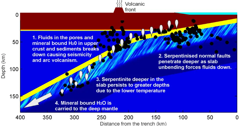
lithospheric mantle is also thought to be hydrated due to normal faulting at the outer rise as the plate bends into the subduction zone (e.g. Peacock, 2001). During subduction the pressure and temperature of the oceanic lithosphere increases causing the hydrous mineral assemblages in the crust to breakdown. It is widely proposed that these metamorphic reactions cause the intermediate depth seismicity seen in subduction zones across the globe through dehydration embrittlement (e.g. Kirby et al., 1996a; Hacker et al., 2003a & b), and that water released from these reactions causes melting within the mantle wedge that leads to the volcanic arc seen above the subducting plate (e.g. Grove et al., 2009).
The hydrated mineral assemblages that are predicted to occur in the subducting slab by thermo-petrological modelling are expected to have much lower seismic velocities than the surrounding mantle material (e.g. Helffrich, 1996; Connolly & Kerrick, 2002, Hacker et al.,
2003 a & b). Seismic studies in a range of subduction zones have detected this low velocity material from converted seismic phases (e.g. Yuan et al., 2000), and more recently high resolution seismic tomography studies (e.g. Zhang et al., 2004).
2 Martin et al., 2003). These seismic phases spend much of their ray path interacting with the low velocity slab, and therefore have the potential to resolve new details of the low velocity structure seen at intermediate depths in subduction zones.
In this study we investigate the resolution of these guided wave phases, and show that guided wave dispersion can not only occur in arrivals from upper plane WBZ seismicity due to low velocity oceanic crust, but can also be seen from lower plane WBZ. We show that dispersive arrivals from the lower plane of the WBZ may be due to low velocity hydrated outer rise normal faults that penetrate the lithospheric mantle. We propose an innovative method for constraining the velocity structure responsible for the guided wave dispersion seen, by comparing the full dispersive waveforms observed in the forearc to synthetic waveforms produced by full waveform simulations.
Using this method we show that upper plane WBZ events are associated with low velocity oceanic crust that becomes less seismically distinct with depth. These observations give the first seismic evidence of dehydration reactions occurring before the onset of full
eclogitization, and confirm that dehydration reactions occur within the subducted crust as predicted by thermo-petrological subduction zone models (e.g. Hacker et al., 2003 a & b; Yamasaki & Seno, 2003). Our observations suggest however that low velocity lawsonite bearing assemblages persist to greater depth than has previously been suggested by thermo-petrological subduction zone models or observations of converted seismic phases.
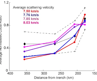
We also show that the subducting lithospheric mantle is hydrated by serpentinised outer rise normal faults. Analysis of the P-wave coda from events in Northern Japan gives an in-situ constraint on the hydration of the lithospheric mantle, increasing the amount of water that is thought to be delivered to the mantle by this subduction zone by an order of magnitude compared to previous studies (e.g. van Keken et al., 2011)
1.1 Motivation and hypothesis
Subduction zone modelling has suggested that hydrous mineral phases in subduction zones not only have a fundamental control on the occurrence of both upper and lower plane WBZ seismicity (e.g. Hacker et al., 2003b), but also have an important role in the global water cycle as subduction transports large amounts of water to the mantle (e.g. van Keken et al.,
3 generally lack the resolution to resolve the predicted mineral phase transformations other than the transformation to high velocity eclogite.
The lack of observational benchmarks for these established subduction zone models is perhaps most apparent in the subducted lithospheric mantle. It is widely suggested that the oceanic lithosphere may be highly hydrated by outer rise normal faulting, but there is little observational constraint on the degree of hydration at intermediate depths. This introduces a large degree of uncertainty to current estimates of the amount of water delivered, especially to the deep mantle (e.g. van Keken et al., 2011)
Guided waves spend longer interacting with the subducted oceanic lithosphere than any other seismic phase. Detailed analysis of guided wave arrivals may therefore be more sensitive to these hydrated subduction zone structures than other seismic techniques.
1.2 Agenda
In this project we present a suite of methods for constraining guided wave arrivals. Direct comparison of the dispersive waveforms recorded in the subduction zone forearc with synthetic waveforms produced by full waveform simulations allows the velocity structure of the WBZ to be tightly constrained. These methods provide a new constraint on the
structures and mineralogies that are associated with upper and lower plane WBZ seismicity, and give the first in-situ estimates of the hydration of the lithospheric mantle.
This thesis is presented in two main parts:
Part one - Modelling and Measuring Subduction Zone Guided Waves Part two - Guided Waves in Subducted Lithosphere
This is prefaced with this introduction and a literature review (Chapter 2). In Chapter 2 we first discuss existing observations linked to WBZ structure, and secondly outline the mineralogies and structures that are predicted by thermo-petrological modelling studies.
In Part one of the thesis the methodologies that are used and developed in this project are discussed. Chapter 3 outlines the Finite Difference (FD) method used to produce synthetic waveforms, and Chapter 4 introduces the methods developed for constraining the
4 Part two of the thesis focuses on the application of these methods to dispersive arrivals observed in subduction zone forearcs. In Chapter 5 we present dispersive arrivals from events that occur well below the upper plane of the WBZ in Northern Japan. This dispersion is proposed to occur due to low velocity serpentinised dipping outer rise normal faults within the subducting mantle lithosphere. Analysis of the P-wave coda from these events gives a new constraint on the degree of hydration of the mantle lithosphere at
intermediate depths, and increases the amount of water estimated to be subducted by this relatively old cool slab by an order of magnitude. This chapter has been accepted for publication in the journal Geology (Garth & Rietbrock, 2014).
In Chapter 6 we present dispersive arrivals recorded in the forearc of Northern Japan from WBZ events at 150 – 220 km depth. Analysis of dispersion from a profile of events from different depths shows that the velocity contrast of the crustal waveguide reduces with depth. This is interpreted as the progressive dehydration of the subducted oceanic crust, and offers the first direct seismological evidence of metamorphic dehydration reactions other than the eclogite transformation. The analysis presented in this chapter suggests that the phase transformations occurring in the Japan subduction zone, including the lawsonite-eclogite transformation occur at greater depths than has previously been suggested. This chapter has been submitted to the Geophysical Journal International.
In Chapter 7 the methodology proposed and results presented are discussed. In particular the significance of these results to our understanding of earthquake processes at
5
Chapter 2
The Wadati-Benioff zone
Anomalously deep seismicity observed beneath volcanic arcs has long been associated with subducted oceanic material. Kiyoo Wadati first suggested that the plane of deep
earthquakes observed beneath Japan may be evidence of ‘continental displacement’ as proposed by Alfred Wegener’s then highly controversial theory of continental drift (Wadati, 1935). Wadati-Benioff zone (WBZ) seismicity is still used as a primary tool for inferring the geometry of subducting slabs. The most recent and comprehensive example of this is the global slab model, slab1.0 (Hayes et al., 2010; 2012).
With increasing instrumentation it has become clear that two distinct layers of WBZ seismicity are seen in many subduction zones. This was first noted in Japan (Umino & Hasegawa, 1975; Hasegawa et al., 1978) and has since been shown to be a common feature of subduction zones across the globe (e.g. Brudzinski et al., 2007). The thickness of the WBZ, and hence the separation of the planes of seismicity has been shown to correlate well with the age of the plate (Brudzinski et al., 2007).
How intermediate (60 – 300 km depth) and deep (> 300 km depth) seismicity occurs, where high temperatures and pressures are thought to inhibit brittle failure, is still not fully understood. The mechanisms proposed must be able to explain the occurrence of upper and lower plane WBZ seismicity in the wide range of temperature and pressure conditions found in subduction zones. There are three mechanisms that are considered as potentially viable explanations for intermediate and deep focus seismicity (e.g. Frohlich, 2006). These are,
1. Dehydration embrittlement
2. Self-localised shear instabilities
3. Transformational faulting
6 Self-localised shear instabilities are an alternative hypothesis that has been proposed to explain intermediate depth seismicity. This hypothesis does not require the production of fluids, and therefore can potentially occur in the absence of hydrous minerals (e.g. Keleman & Hirth, 2007). Seismicity is proposed to occur as shear instabilities increase the heat locally, reducing the viscosity and producing a self-localising feedback mechanism that allows brittle failure to occur (e.g. John et al., 2009).
Transformational faulting has mainly been suggested as an explanation for deep focus earthquakes. It is proposed that at these depths seismicity occurs due to the phase change of olivine to modified spinel or wadsleyite (e.g. Kirby et al., 1996b; Stein & Stein, 1996). The phase change is proposed to occur in the transition zone in older, quickly subducting and therefore cooler slabs, where meta-stable olivine persists to greater depths. This theory potentially explains why deeper earthquakes are generally associated with subduction zones where cool lithosphere is subducting quickly (e.g. Frohlich, 2006).
As is discussed in the second part of this chapter (section 2.2), it has been widely shown that the occurrence of intermediate depth seismicity correlates well with the expected occurrence of hydrous mineral assemblages in the WBZ (e.g. Hacker et al., 2003b). While transformational faulting and self-localised shear instabilities cannot be ruled out as a potential mechanism by which intermediate depth seismicity may occur, it is widely accepted that dehydration of hydrous minerals can account for the intermediate depth seismicity seen in subduction zones.
Hydrous mineral assemblages proposed to occur in the WBZ provide potential a mechanism for intermediate depth seismicity, a source of water causing mantle melting and arc
volcanism, and an explanation for low velocity structures that are seen in the subducting slab. In the first part of this chapter the seismic observations suggesting that low velocity hydrous mineralogies may be present at depth will be discussed. In the second part we will discuss the thermal and petrological modelling methods used to estimate what mineral phases could explain the occurrence of WBZ seismicity, arc volcanism, and the observed low velocity structures.
2.1 Inferring and imaging low velocity structure in the WBZ
7 smaller scale low velocity features may be seen on top of subducting slabs (e.g. Helffrich & Abers, 1997). These low velocity structures have been inferred by a range of seismological techniques including the observation of subduction zone guided waves (e.g. Abers, 2000) and converted seismic phases (e.g. Matsubara et al., 1986). With increasing network coverage in many subduction zones these low velocity features have also been imaged by receiver function techniques (e.g. Yuan et al., 2000) and high resolution seismic
tomographic studies (e.g. Zhang et al., 2004). In this section these observations are briefly summarised.
2.1.1 Guided waves observations in subduction zones
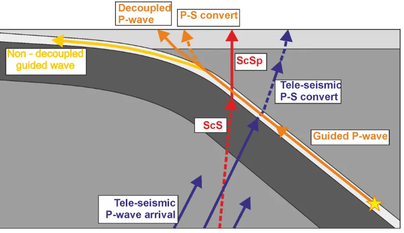
Observations of dispersed P-wave arrivals (e.g. Abers, 2000), focusing of high frequency energy (e.g. Martin, et al., 2003; Furumura & Kennett, 2005) and extended P-wave coda (Furumura & Kennett, 2005) have widely been attributed to the presence of a low velocity waveguide associated with WBZ events. Dispersed waveforms that have been attributed to these subduction zone waveguide structures have been observed across the globe. Guided wave dispersion occurs as high frequency, short wavelength seismic energy is retained and delayed in the low velocity oceanic crust, while low frequency longer wavelength energy travels in the faster surrounding material.
Generally guided wave dispersion is seen in the subduction zone forearc, where high frequency guided wave energy has decoupled due to the bend of the slab (Martin et al.,
2003). Non-decoupled guided wave arrivals have however also been seen at ocean bottom seismometers close to the trench in Northern Japan (Shito et al., 2013).
Body wave dispersion associated with a low velocity waveguide has been observed at many subduction zone across the globe including Northern Japan (e.g. Abers 2000; 2005;
Furumura & Kennett 2005), Alaska and the Aleutians (Abers & Sarker, 1996; Abers, 2005), Nicaragua (Abers, 2003), South America (e.g. Martin et al., 2003; Martin & Rietbrock, 2006), the Hellenic arc (Essen et al., 2009) and Southeast Japan (e.g. Hori et al., 1985; Miyoshi et al., 2012). This wide range of observations suggests that the low velocity structure is a common feature in many subduction zones. For dispersion to occur the source must be on or very near to the waveguide (Abers, 2005; Martin & Rietbrock, 2006), suggesting that these low velocity structures may be directly associated with the occurrence of
8 Subduction Zone Approximate
slab dip
Velocity of LVL (km/s) Inferred from GUIDED
WAVES
Inferred from other methods
Central Andes ~16⁰ a ~ 7.5 a -
Cascadia ~21⁰ b - -
Japan ~26⁰ c 7.72 – 7.95 e 6.2 – 7.0 f
Alaska ~33⁰ b 4.10 – 7.97 e 4.6 – 6.1 g
Nicaragua ~45⁰ d 7.66 – 7.87 e -
Table 2.1 – Comparison of LVL velocities and slab dip, from guided wave and other studies. Figures are taken from the following references, a Martin & Rietbrock (2006), b Rondenay et al. (2008), c Kawakatsu & Watada, (2007), d Mackenzie et al. (2010), e Abers, (2005), f Nakajima et al. (2009), g Ferris et al. (2003).
In most cases guided wave dispersion is attributed to a low velocity layer (LVL) of 2 – 8 km thickness that is 5 - 8 % slower than the surrounding material (e.g. Abers 2000; Martin et al., 2003). The variation in waveguide velocity contrast seen in the Pacific subduction zones studied by Abers (2005) correlates well with the dip of the slab, with steeper subduction zones showing a greater velocity contrast. This data is shown in table 2.1, and is compared with velocities inferred from other seismic studies. It is proposed that this greater velocity contrast is due to released fluids being channelled up dip more effectively in steeper subduction zones (Abers, 2005). Abers (2005) also suggested that guided waves from events at greater than 150 km depth may see a smaller velocity contrast than events occurring above 150 km.
One notable exception is arrivals from intermediate depth events in the Tonga subduction zone which show a high frequency first arrival, and delayed low frequency arrivals (e.g. Gubbins & Snieder, 1991). It is proposed that this dispersion occurs due to a high velocity layer of eclogitized crust (Gubbins et al., 1994). It is also possible that the long ray paths of the observed waveforms in this study means that deeper eclogitized slab structure is sampled, causing the high frequency early arrival.
9 adopted by several later studies, and averaged dispersion curves have been used to
quantify the low velocity waveguides in Pacific subduction zones (Abers, 2005).
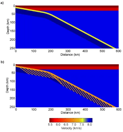
Martin et al. (2003) also note that the high frequency component of the waveform is delayed, and that guided wave arrivals are associated with a characteristic high frequency peak when the signal is plotted in the frequency domain. Martin et al. (2003) use two-dimensional (2D) waveform simulations to show that a low velocity waveguide can explain the guided wave observations made in the South American subduction zone. The resulting waveforms are controlled not only by the velocity and width of the waveguide, but also by the source offset and slab geometry (Martin & Rietbrock 2006). Other works have since used 2D waveform simulations to show that these observations can be explained by energy escaping a low velocity waveguide (e.g. Essen et al., 2009, Miyoshi et al., 2012), and that guided wave energy can be seen by ocean bottom seismometer close to the trench (Shito
et al., 2013). The approximate ray paths of these guided wave phases in the slab are shown schematically in figure 2.1.
[image:16.595.116.527.482.719.2]Furumura & Kennett (2005) show that a single LVL cannot alone account for the extended P-wave coda that is seen in the North of Japan. They use 2D waveform propagation models to explore the seismic structures that may lead to the extended P-wave coda, and conclude that random scatterers, elongated parallel to the slab can cause the extended P-wave coda seen where a LVL is also present.
10 Subduction zone waveguide effects have also been investigated using three-dimensional (3D) waveform simulations (e.g. Shapiro et al., 2000, Furumura & Kennett, 2005) but these models generally lack the resolution required to fully model waveguide effects at the required scale length.
2.1.2 Converted seismic phases in subduction zones
Converted seismic phases have been used to infer low velocity structures associated with the subducting slab. P-S conversions were first noted along the Fiji-Tonga trench by
Mitronovas & Isacks (1971), who attributed the arrival to a sharp boundary at the top of the slab. Precursors to ScS arrival (ScSp) seen in Japan (Okada, 1971) and South America (Snoke
et al., 1977) are thought to occur due to an S-P conversion which is also attributed to a sharp velocity change at the top of the slab.
Matsuzawa et al. (1986) showed that P-S conversions in Northern Japan were explained well by a 6 % slow LVL with a thickness of 10 km or less, lying above a high velocity slab that is 6 % faster than the surrounding mantle material. Similar observations in the Eastern Aleutians have shown that P-S conversions here can be explained by a LVL that is approximately 8 % slower than the surrounding material (Helffrich & Abers, 1997).
Teleseismic P-S conversions observed at large temporary and permanent seismic networks have been used to image the velocity structure of subducting slabs at a variety of
subduction zones. These receiver function studies can be used to image sharp velocity contrasts in the Earth, and are sensitive to relatively small scale low velocity structures in the subduction zone. The ray path of these converted phases is shown schematically in figure 2.1. In the central Andes receiver function studies using data from a range of dense temporary seismic networks have shown a sharp reflector associated with the intermediate depth seismicity, that is interpreted as a 5 - 10 km thick LVL with an S-wave velocity
contrast of ~15 % (Yuan et al., 2000). The conversion signal terminates at ~120 km depth and is interpreted as metastable non-eclogitised mafic crust that becomes fully eclogitised at 120 km depth, and hence is no longer seismically detectable. While much of the
intermediate depth seismicity occurs within the LVL, Yuan et al. (2000) also note that some seismicity occurs 10 - 20 km below the LVL in the subducted oceanic mantle.
11 hydrous minerals in the subducting oceanic crust, persists to a depth of ~100 km, below which a velocity increase with depth is imaged. Kawakatsu & Watada (2007) postulate that as the low velocity oceanic crust becomes less hydrated, the released water forms a layer of low velocity serpentinite above the subducting slab. Therefore an increase in velocity is seen with increasing depth as the underlying oceanic crust has a higher velocity than the proposed layer of low velocity serpentinite. To date however no such structure has been proposed in other subduction zone settings.
Receiver function methods have however suggested the presence of low velocity
subducted oceanic crust at a variety of other subduction zones including Alaska & Cascadia (e.g. Rondenay et al., 2008). In general these studies show that the LVL is 5 - 10 km thick, with the exception of the Alaskan subduction zone which is thought to be much thicker possibly due to the subduction of the thicker oceanic crust associated with the subducting Yakutat terrain (Ferris et al., 2003).
These studies show that the LVL persist to 100 - 120 km in most subduction zones, below which it is no longer seismically observable (in receiver function studies) presumably due to the onset of full eclogitization. The exception to this is the Cascadia subduction zone where the LVL is thought to terminate at ~40 km due to the high temperatures of the young subducting crust (Rondenay et al., 2008). The depths to which receiver function methods resolve the oceanic LVL are persistently shallower than the depth to which guided wave studies infer low velocity structure to exist in the same subduction zones, as is summarised in table 2.2. It is also noted that some guided wave studies have suggested that the LVL may be less than the 5 km lower bound of thickness inferred for receiver function studies (e.g. Martin et al., 2003).
2.1.3 High resolution seismic tomography
12 Subduction zone Approximate age of subducting plate(Myr)
Depth extent of LVL (km) from RECEVIER FUNCTION studies from GUIDED WAVE studies Cascadia Nicaragua Alaska Central Andes Japan 10 30 50 60 150 40a 100b 120-130a 120c 100-120d - 150e 250f 160 - 250g
~250f
Table 2.2 – Depth of LVL inferred from different methods. Plate ages are based on Müller et al.
(2008). Depths inferred from the following references a Rondenay et al. (2008); b Mackenzie et al.
(2010); c Yuan et al. (2000); d Kawakatsu & Watada (2007); e Abers et al. (2003); f Abers (2005); g Martin et al. (2003).
Zhang et al. (2004) showed a reduced P-wave velocity associated with both the upper and lower planes of seismicity as well as a reduced S-wave velocity associated with the upper plane of seismicity. Similar observations have since been made in the Hokkaido region of Northern Japan using a travel time tomography with an exceptionally large data set
(Nakajima et al., 2009). This study also shows reduced P-wave and S-wave velocities in both the upper and lower seismic planes (Nakajima et al., 2009).
Nakajima et al. (2009) interpret the lower plane low velocity anomalies as serpentinite or a chlorite bearing Harzburgite. Zhang et al. (2004) rule out serpentinite as they do not observe an S-wave velocity anomaly associated with the lower plane of seismicity, and instead propose that a forsterite-enstatite-H20 formation may cause the reduced P-wave velocities observed. These two studies offer the first direct observations suggesting that hydrous mineral assemblages are present in the lower plane of seismicity. This suggests that dehydration embrittlement could potentially account for lower plane as well as upper plane WBZ seismicity.
Low velocity structure relating to the lower plane of seismicity has been imaged by
tomographic studies in Northern Chile (Dorbath et al., 2008) and Central America (Syracuse
et al., 2008), although both of these studies lack the resolution to determine if this low velocity structure forms a separate LVL, or is directly related to the lower plane of
13 features may be present at other subduction zones where tomographic studies with the necessary resolution are not currently possible.
2.1.4 Observations of outer rise normal faulting
Outer rise normal faulting potentially has an important control on the hydration of subducting material. Several studies have suggested that the oceanic mantle may be hydrated by outer rise faults allowing lower plane WBZ earthquakes to occur by dehydration embrittlement (e.g. Peacock, 2001). It has also been suggested that this hydration could potentially transport large amounts of water to the mantle (e.g. van Keken
et al., 2011).
The surface expression of outer rise normal faulting is apparent in many subduction zones, where fault scarps are seen running roughly parallel to the trench. In Central America these outer rise faults have been imaged by seismic reflection to greater than 20 km depth (Ranero et al., 2003). Tomographic inversion of reflected and refracted waves from this survey show that this outer rise faulting is also associated with a reduction in seismic velocity as the plate bends into the trench (Ranero et al., 2004).
The onset of outer rise faulting has also been shown to correlate with a decrease in heat flow (Grevemeyer et al., 2005), and magnetotelluric studies have shown an increase in conductivity close to the trench in Central America (Worzewski et al., 2012). These observations are thought to represent the onset of hydration and serpentinisation of the oceanic mantle due to the normal faulting occurring at the outer rise.
These observations do not however constrain the depth to which the subducting plate is hydrated at the outer rise. Passive seismic tomography performed offshore Nicaragua shows that the maximum depth at which reduced velocities occur corresponds to the maximum depth at which normal faulting micro-earthquakes are detected (Lefeldt et al.,
2012), providing further evidence that hydration at the outer rise occurs due to normal faulting.
It should be noted that many of the studies directly quantifying the hydration of the oceanic mantle at the outer rise have been conducted at the Nicaraguan trench.
14 In South and Central America it has been shown that focal mechanisms of outer rise
earthquakes have a similar orientation with respect to the oceanic plate as intermediate depth events occurring within the WBZ (Ranero et al., 2005). Ranero et al. (2005) therefore propose that outer rise normal faults may be reactivated at depth, accounting for much of the intermediate depth seismicity seen in these subduction zones.
The hypothesis that intermediate and deep focus earthquakes occur on pre-existing faults such as outer rise faults has been tested in several subduction zones using the methods of Warren & Silver (2006) to determine the fault plane of intermediate and deep earthquakes. Warren & Silver (2006) propose that the rupture orientation of intermediate and deep focus earthquakes can be determined by considering the length of the rupture at different stations, as the shortest rupture lengths will be seen where the ray path to the station is approximately parallel to the rupture direction.
Warren et al. (2008) confirm that in Central America events at depths between 35 and 85 km depth occur on reactivated outer rise normal faults. Studies using this method in the Tonga-Kermadec subduction zone (Warren et al., 2007) and the Izu-Bonin-Marianas
subduction zones (Myhill & Warren, 2012) conclude that pre-existing fault structures do not control the orientation of intermediate and deep fault planes. The relationship between outer rise faulting and intermediate depth seismicity is not fully understood, but appears to be a control on intermediate seismicity in some but not all subduction zones.
2.1.5 Summary of observations
Low velocity structures exist at intermediate depth in many subduction zones, and are widely interpreted as subducted oceanic crust. Earthquakes can occur both within the low velocity oceanic crust and several kilometres below it in the oceanic mantle. Low velocity structures persist to depths of 40 – 250 km depending on the subduction zone. At greater depths these structures are seismically indistinguishable which is interpreted as the onset of full eclogitization. There is however a discrepancy between the depth to which low velocity material is imaged by receiver function methods, and the depths to which it is inferred by guided wave studies, with subduction zone guided wave observations
15 Other low velocity structures have been inferred and imaged such as a layer of serpentinite above the slab (Kawakatsu & Watada, 2007), and a lower LVL associated with the lower plane of seismicity (Zhang et al., 2004; Nakajima et al., 2009). This imaged lower LVL provides an explanation of how intermediate depth seismicity may occur on the lower seismic plane through dehydration embrittlement. A widely proposed explanation of how this hydration of the mantle can occur to these depths is through normal faults that penetrate the oceanic mantle at the outer rise. The fault scarps of normal faults are apparent at the outer rise of many subduction zones and a range of observations have suggested that hydration of the incoming plate may occur here.
2.2 Modelling hydration of the WBZ
As direct observations of the WBZ are limited much of our understanding of processes occurring at these depths is informed by numerical simulations of conditions found during subduction. Thermal models have been used to calculate the temperature and pressure conditions expected in subducting plates at WBZ depths, and petrological modelling has been used to determine the metamorphic phases that may be stable at these conditions. In this section we discuss how various modelling methods have been used to simulate the hydration and dehydration of the subducting oceanic plate.
2.2.1 Hydration of the oceanic lithosphere
It is widely expected that the oceanic crust is hydrothermally altered as oceanic water convects through the crust as it cools, forming features such as black smokers (e.g. Fowler, 2005). This process can only conceivably hydrate the upper few kilometres of the
lithosphere. Lower plane WBZ seismicity and associated velocity anomalies however have both been attributed to the presence of hydrous mineral assemblages up to 40 km below the top of the slab in the subducted oceanic mantle.
16 Ranero et al., 2004), resistivity (e.g. Worzewski et al., 2011) and heat flow (e.g. Grevemeyer
et al., 2005), as summarised in part 2.1.
Numerical simulations of how water interacts with the subducting slab have shown that normal faults forming at the outer rise as the plate bends can act as a fluid pathway, allowing hydration of the subducting oceanic mantle (Faccenda et al., 2009). As the plate unbends a downward pressure gradient on the fault zone forces fluids to greater depths (Faccenda et al., 2012). This mechanism suggests that hydrated mineral assemblages may form along fault zone fluid pathways in the subducting oceanic mantle.
These simulations also show that the water transported along these fault zone fluid pathways may form a hydrated layer within the oceanic mantle, as well as a hydrated layer at the top of the slab (Faccenda et al., 2012). This double hydrated zone has a similar separation to the double seismic zones of older subducting plates. It is also noted that these double hydrated zones bear a striking resemblance to the double low velocity zones seen in high resolution tomographies of Northern Japan (e.g. Zhang et al., 2004; Nakajima
et al., 2009). Faccenda et al. (2012) propose that the two modelled hydrated zones can account for the two layers of WBZ seismicity seen in many subduction zones, and suggest that the lower layer of WBZ seismicity occurs due to hydro-fracturing as buoyant fluids in the lower hydrated zone percolate up dip. This contrasts with the widely proposed view that lower plane seismicity can be explained by the breakdown of hydrous mineral assemblages in the subducting oceanic mantle (e.g. Peacock, 2001). It has however also been suggested that the breakdown of hydrous minerals formed by outer rise fault hydration can explain the variation in separation of the two planes of WBZ seismicity (e.g. Iyer et al., 2012).
2.2.2 Dehydration of the subducting slab
17
Hydrous mineralogies and intermediate depth seismicity
The three main hypotheses of how intermediate depth seismicity can occur at subduction zones are outlined at the start of this chapter. The most widely proposed and supported of these theories is that intermediate depth seismicity occurs due to dehydration
embrittlement, where the breakdown of hydrous mineral assemblages allows brittle failure to occur. This would suggest that hydrous mineral assemblages would be expected to be present, and undergoing dehydration reactions at the depths at which seismicity occurs. Thermal and petrological modelling to determine where hydrous minerals may occur in the subduction zone has therefore been a key tool in assessing the viability of intermediate depth seismicity occurring through dehydration embrittlement.
It is widely proposed that upper plane WBZ seismicity occurs due to the dehydration of meta-basalt (and meta-gabbros) as they transform to eclogite (e.g. Kirby et al., 1996a). It has also been shown that the lower plane of seismicity can be explained by the breakdown of serpentine formed in the subducting oceanic mantle by hydration due to outer rise faulting (Peacock, 2001). Yamasaki and Seno (2003) showed that the dehydration of antigorite and mid-ocean ridge basalt (MORB) can potentially explain the variation in thickness of the WBZ in several pacific subduction zones.
Hacker et al. (2003a) considered a suite of compositions found in the subduction oceanic plate, and produced pressure-temperature (P-T) plots for crustal compositions (e.g. MORB), as well as compositions found in the oceanic mantle such as depleted and un-depleted lherzolite, harzburgite and serpentinite. Using this data set Hacker et al. (2003b) calculated the occurrence of hydrous mineral assemblages in Pacific subduction zones and showed that intermediate depth seismicity correlates well with where hydrous mineral assemblages are expected to occur in the subducting slabs. Coupled with the seismic observations of low velocity minerals in the subducting slab, this provides strong evidence that intermediate depth seismicity occurs in the presence of hydrous mineral assemblages. It is therefore likely that intermediate depth seismicity in subduction zone occurs due to dehydration embrittlement.
18 transition, while in hot subduction zones dehydration occurs due to the zoisite-eclogite transition. Lawsonite breakdown is associated with a net volume increase, while zoisite breakdown is associated with a net volume decrease meaning there is no increase in pore fluid pressure. Therefore zoisite breakdown may not cause seismicity in the crust.
Serpentinite breakdown is thought to control seismicity in the subducted oceanic mantle in both settings. This is proposed as an explanation for the observations of Abers et al. (2013), who compile high resolution seismic images and accurate earthquake locations to show that intermediate depth seismicity occurs within the oceanic crust in old subduction zones, and beneath it in young subduction zones.
Low velocity mineral assemblages
The wide range of seismic observations of low velocity structure associated with the subducting slab outlined in section 4.1 gives further evidence that there may be hydrous mineral assemblages present at depth in subduction zones. In order to properly interpret the low velocity anomalies that are observed it is important to understand the seismic properties of the candidate mineralogies that can be expected at the depths (e.g. Helffrich, 1996). A number of hypotheses have been proposed to explain the observed low velocity anomalies.
1. The presence of meta-stable gabbro has been considered by several studies. This hypothesis is however widely rejected as the persistence of gabbro would require almost completely anhydrous conditions during subduction, and the predicted velocity contrast for anhydrous gabbro is higher than is observed (e.g. Abers 2005, Connolly & Kerrick 2002).
2. A layer of serpentinised mantle material above the slab has been proposed to explain receiver function images in Northern Japan (e.g. Kawakatsu & Watada, 2007), but is not considered a viable explanation for LVLs imaged by receiver functions in other subduction zones (e.g. Rondenay et al., 2008). Observations of guided waves resulting from LVL structure in subducting slabs do not favour this hypothesis either, as for guided wave dispersion to be seen the source must be on or near to the low velocity waveguide (e.g. Abers, 2005; Martin & Rietbrock, 2006) and it is unlikely that strain would localise within a layer of serpentinite.
19 images has also show that intermediate depth earthquake sources occur in the subducting oceanic crust in cool slabs, or below the moho in warmer slabs (Abers et al., 2013). This also suggests that guided wave energy is unlikely to be excited in a LVL above the slab.
3. It has also been suggested that free fluid phases occurring within the slab at
intermediate depths may cause the observed velocity decrease. It is however noted that this would require a larger amount of fluids than is expected to occur in the subduction setting (e.g. Abers, 2005).
4. By far the most widely accepted hypothesis to explain the low velocity slab structures is that hydrated phases within the subducted mafic crust persist to depths of 100 – 250 km depending on the subduction conditions (e.g. Connolly & Kerrick, 2002; Hacker et al., 2003b). This hypothesis is discussed in further detail below.
Connolly & Kerrick (2002) note that lawsonite “has a profound effect on seismic velocities”.
Phase diagrams of altered (and un-altered) MORB compositions calculated by free energy minimization show that lawsonite persists to high temperatures ( > 700⁰c at 7.5 GPa) and extremely high pressures ( > 9 GPa), and therefore may account for the low velocities seen in the slab at these conditions (Connolly & Kerrick, 2002).
Hacker et al. (2003a) perform similar calculations for the bulk compositions of the oceanic crust (e.g. MORB) and mantle (e.g. harzburgite, lherzolite and serpentinite). The predicted velocity of the mineral phases present at intermediate depths are then calculated, showing that low velocity hydrous minerals are expected to occur in the WBZ at a range of
subduction conditions (Hacker et al., 2003b). The termination of the LVL is then proposed to correspond to the breakdown of lawsonite. Connolly & Kerrick (2002) propose this is due to the stishovite transition in cool subduction zones, and due to the lawsonite-coesite transition in warmer subduction zones. Hacker et al. (2003a & b) however suggest that the termination of the LVL corresponds to the lawsonite-eclogite transition.
20 subduction zones using the methods of Peacock (1990), and suggest a less steep P-T path even for cool subduction zones.
Thermal modelling suggests that the breakdown of lawsonite to eclogite controls the termination of the LVL in warmer subduction zones (e.g. Hacker et al., 2008), and this phase transformation has been shown to correlate well with observations in Cascadia and Alaska (Rondenay et al., 2008). However the termination of the LVL due to other transitions identified by Connolly and Kerrick (2002) cannot be ruled out, especially for cooler subduction settings.
Water delivered to the Earth’s mantle
The Earth’s oceans are thought to have originally been derived from the juvenile hydrated mantle (e.g. Rüpke et al., 2006). At subduction zones oceanic water contained in hydrous mineral assemblages is returned to the mantle. The water transported to the mantle during subduction is likely to play a major role in the global water cycle, and it is therefore
important to understand how much water is transported in subducted hydrous mineral assemblages. The thermal and petrological methods that have been used to determine if intermediate depth seismicity occurs through dehydration embrittlement, and if low velocity anomalies can be explained by hydrous mineral assemblages, can also be used to address the amount of water that is transported during subduction.
Arguably the most complete study of this kind is that of van Keken et al. (2011) who take the metamorphic relationships derived by Hacker (2008), and the global compilation of slab thermal models of Syracuse et al. (2010) to produce a detailed estimate of the amount of water transported to the mantle at subduction zones globally. Van Keken et al. (2011) calculate the water content of oceanic sediments and estimate that the 8 Tg/Myr of oceanic water is subducted by the oceanic crust. Approximately 10 % of this water is carried in the sediments, and so is likely to be lost at shallow depths (van Keken et al.,
2011). The remaining 90 % is carried in crustal basalt and gabbro, and is lost at a range of intermediate depths depending on the thermal conditions of the subduction zone. Overall van Keken et al. (2011) propose that ~69 % of water subducted globally by the oceanic crust is lost to the oceanic mantle at depths of less than 230 km, with ~31 % being transported to the deeper mantle. Hydrated crustal rocks break down at shallower depths in hot
21 In this study van Keken et al. (2011) simply approximate the hydration of the subducting oceanic mantle as a 2 km thick layer of serpentinised mantle material that is 2 wt% hydrated, reflecting the large amount of uncertainty that exists in the overall hydration of the subducting oceanic mantle. Van Keken et al. (2011) also quote the H2O flux assuming a fully serpentinised slab mantle, and an un-serpentinised slab mantle highlighting the important role of slab mantle hydration in the global water cycle.
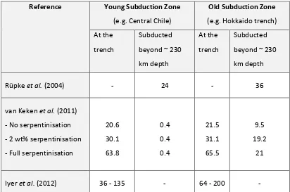
It is proposed that the lithospheric mantle can carry large amounts of water to the deep mantle (e.g. Rüpke et al., 2004; Iyer et al., 2012), and the lack of observational constraint on this hydration is the largest source of error in current models of the global water cycle (e.g. van Keken et al., 2011). Subducting mantle hydration may be particularly important for understanding the amount of water transported to the deep mantle, as it has been
suggested that up to 40 % of slab mantle hydration may be delivered to the deep mantle in cool slabs, by high pressure hydro-silicates such as phase-A serpentinite (Rüpke et al.,
2004).
The hydration of the lithospheric mantle therefore dominates the water delivered to the deep mantle. Rüpke et al. (2004) consider the amount of water subducted by the oceanic mantle, as well as the crust and sediments to calculate the amount of water delivered to the mantle over the age of the Earth, concluding that present day mantle hydration is dominated by recycled oceanic water rather than residual juvenile hydration.
It is not fully understood if water can be delivered to the transition zone through a continuous chain of hydrous silicates. It has however been suggested that not all water released from dehydration reactions is released to the mantle, but some water may be transported to deeper within the slab due to downward pressure gradients on normal faults penetrating the lithospheric mantle (Faccenda et al., 2012). This water may then be transported to the transition zone regardless of the stability of hydro silicates.
Iyer et al. (2012) use a reactive flow model to estimate the hydration of the oceanic mantle at subduction zones with a variety of subduction parameters, and benchmark these
estimates to observations of hydration at the outer rise in South and Central America. They show that the oceanic mantle is likely to be highly hydrated, and therefore able to transport large amounts of water to the mantle, especially in cooler subduction zones. The amount of water that is estimated to be delivered to the deep mantle by various studies is
22 Reference Young Subduction Zone
(e.g. Central Chile)
Old Subduction Zone (e.g. Hokkaido trench) At the
trench
Subducted beyond ~ 230 km depth
At the trench
Subducted beyond ~ 230 km depth
Rüpke et al. (2004) - 24 - 36
van Keken et al. (2011) - No serpentinisation - 2 wt% serpentinisation - Full serpentinisation
20.6 30.1 63.8 0.4 0.4 0.4 21.5 31.1 65.5 9.5 19.2 21
[image:29.595.106.518.69.342.2]Iyer et al. (2012) 36 - 135 - 64 - 200 -
Table 2.3 – Comparison of estimates of mineral bound H2O is the subducting plate. Amounts subducted quoted in Tg/Myr/m of arc. Estimates from Rüpke et al. (2004) assume plate subducting at 6 cm/yr. Otherwise plate age and rate of subduction is based on van Keken et al. (2011).
2.3 Summary
Low velocity structures imaged by a range of seismic techniques can be explained by hydrous mineral assemblages that occur at the temperature and pressure conditions found during subduction. The upper LVL is thought to consist of meta-stable basaltic material, with the identifiable low velocity phases correlating roughly with the persistence of lawsonite (Connolly & Kerrick, 2002; Hacker et al., 2003a & b).
The patterns of intermediate depth seismicity seen in Pacific subduction zones correlates well with the predicted occurrence of hydrous mineralogies (e.g. Hacker et al., 2003b). This strongly supports the hypothesis that dehydration embrittlement is the dominant
mechanism by which intermediate depth seismicity occurs.
The lower LVL structure associated with the lower plane of seismicity (e.g. Zhang et al.,
23 The low velocity minerals associated with WBZ seismicity and reduced seismic velocities in the slab also have the potential to transport large amounts of water to the mantle. Thermal petrological models (e.g. van Keken et al., 2011) have given a good approximation of water transported by the upper slab, and it is proposed that the hydrated subducting oceanic mantle transports large amounts of water especially to the deep mantle (Rüpke et al.,
2004). The lithospheric mantle is widely thought to be highly hydrated due to outer rise faulting, though the degree of hydration is poorly constrained. This is a major source of uncertainty in current estimates of the total H2O flux to the mantle (e.g. van Keken et al.,
2011).
Finally we highlight three main features of the WBZ that are not fully understood.
1. Thermal petrological modelling (e.g. Peacock et al., 2001) and fluid flow modelling (e.g. Faccenda et al., 2012) suggest that the lower plane of seismicity may occur due to the presence of fluids introduced at these depths by outer rise faulting. There is however currently no observation evidence that these outer rise normal faults occur at
intermediate depths.
2. Hydration of the subducting lithospheric mantle due to these outer rise normal faults may also be responsible for a large amount of the water that is delivered to the mantle, and especially the deep mantle. There are however currently no observational
constraints on the degree of hydration of the lithospheric mantle at intermediate depths.
3. Though it is widely proposed that the termination of the LVL correlates with the onset of full eclogitization (e.g. Rondenay et al., 2008) the depth at which is inferred to occur by receiver function methods differs from the depths inferred from guided wave studies. There also little seismic evidence of the velocity changes associated with other phase changes in the subducting slab.
24
Part one
Modelling and Measuring Subduction
25
Chapter 3
Waveform Modelling Using the Finite
Difference Method
In this thesis numerical models are used to simulate dispersed and scattered P-wave arrivals from Wadati-Benioff zone events, which are observed globally in subduction zone forearcs. Synthetic waveforms are produced using the finite difference (FD) method to simulate both elastic and visco-elastic properties of the subduction zone structure. Modelling is carried out with two and three dimensional (2D and 3D) models using the staggered grid FD method implemented in sofi2D and sofi3D (Bohlen, 2002).
In this chapter the formulation of the FD method is described, with particular emphasis on the methods that are relevant to this study. Firstly the elastic case is considered, before introducing the formulation of the visco-elastic case. The formulation of the free surface, and absorbing boundary conditions used are then summarised. The source implementation and stability criteria of the method are then described. The specific model setup and variables used are described in Chapter 4.
3.1 The Elastic Case
26 ( ) ( ) ( ) ( ) ( ) ( )
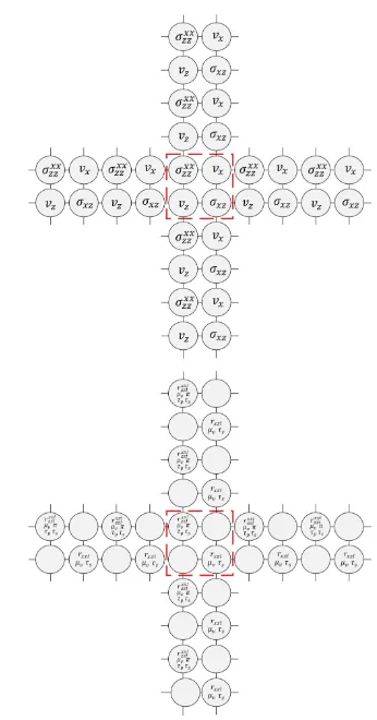
The velocity-stress scheme introduced by Virieux (1986) was implemented using second-order Taylor coefficients on a staggered grid. This method was modified for a fourth-second-order staggered grid by Lavander et al. (1988). The fourth-order staggered grid means that a given wavelength is in effect sampled twice as many times, and therefore a coarser grid spacing can be used for a given resolution frequency. The geometry of the 2D fourth-order staggered grid for the velocity-stress scheme described by Lavander et al. (1988) is
summarised in figure 3.1a. In this project a fourth-order staggered grid is used in all model setups. In order to model wave propagation in 3D using a FD scheme the velocity and stress in the -direction must be introduced. The velocity-stress FD scheme for the 3D case is shown below following Graves (1996).
27 ( ) ( ) ( )
3.2 The Visco-Elastic Case
While the elastic case is useful for modelling the velocity structure we know that the Earth does not deform entirely elastically, and that some seismic wave energy is taken up through viscous deformation. This is potentially important in subduction zones where the seismic quality factor can vary from as little as 30 in the mantle wedge compared to 1000 in the cool subducting lithosphere (e.g. Tsumura et al., 2000; Rychert et al., 2008).
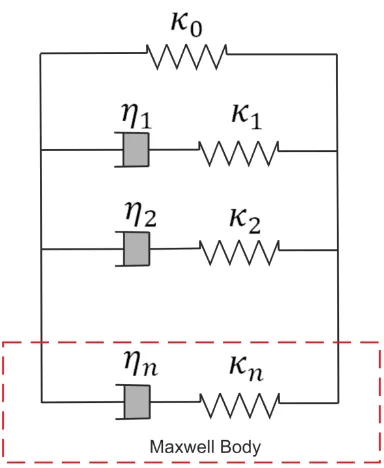
The viscous deformation is introduced to the FD model by considering a series of Maxwell bodies, or dashpots, as shown in figure 3.2. This approach introduced by Emmerich & Korn (1987) takes parallel Maxwell bodies ( ) in series with a spring ( ) to describe the viscous rheology. The elastic rheology is described by a single spring ( ) in parallel with the Maxwell bodies, giving a visco-elastic body that is described as a generalised standard linear solid (GSLS) (Emmerich & Korn, 1987; Bohlen, 2002). From these bodies we can then define the stress relaxation time ( ) and the strain relaxation time ( ) following Bohlen (2002),
( )
is constant over the frequency range of seismic waves that are considered in this study, but a single Maxwell body does not give a that is constant in the frequency domain. A series of Maxwell bodies can however be used to approximate a constant in the
29 Figure 3.2 – Approximation of a visco-elastic body using Maxwell bodies. Modified from Emmerich & Korn, (1987) and Bohlen, (2002).
where is defined following Blanch et al. (1995) as,
( )
The variable was introduced by Blanch et al. (1995) to reduce the amount of memory required as well as the number of calculations needed to simulate a Maxwell body. Varying the value allows a given value of to be determined, while the frequency range for which
is approximated is controlled by the stress relaxation times ( ) (Blanch et al., 1995). In a
medium where the P-wave and S-wave quality factor and respectively are different, is defined for both P and S waves. The stress relaxation time is however the same for both and . Therefore the visco-elastic properties of a given medium can be described by the parameters , and , where,
( )
In order to model the response of these viscous bodies in the FD model, we must
30 is analogous to the term ( ) in the elastic case, while is analogous to the Láme parameter . The values of and are defined below following Bohlen (2002).
( √ ∑ ) ( ) ( √ ∑ ) ( )
Where is the real part of the expression, is the centre frequency of the model domain, and and are the P and S wave velocities at this frequency respectively
(Bohlen, 2002). These variables are then incorporated into the 2D FD scheme following Robertsson et al. (1994) as shown below. The velocity terms remain the same as in the elastic case (equation 3.1), but the stress variables are modified. The memory variables ,
and are also introduced and correspond to the stress variables and
respectively. The distribution of the extra variables considered in the 2D visco-elastic case is shown in figure 3.1b.
31 ( ( ) ( ) ( ) ) ( ( ) ( ) ( ) ) ( ( ) ( ))
3.3 Boundary Conditions
The FD model used here is a block model, and so we must consider how to treat
boundaries. The top of the model is described as a free surface, as is the case on Earth. The bottom and sides of the model however are described as absorbing boundaries, which do not reflect seismic energy, and so a pseudo-infinite medium is simulated. Two methods of implementing an absorbing boundary are discussed below,
1. Perfectly Matched Layers (PML) 2. Exponential Dampening
Both methods effectively dampen the wavefield in an absorbing layer that simulates the infinite boundary as shown in figure 3.3. The formulation of the free surface, as well as both methods of approximating an absorbing boundary condition are considered below.
32
3.3.1 The free surface
At the top of the model (z = 0) a free surface is implemented following Lavender et al.
(1988) where the vertical stress components ( and ) at the top of the model are
mirrored across the top surface ( ). The horizontal stress component ( ) is not
modified. In order to allow for the staggered grid implementation the stresses are considered to be symmetrical about the surface (z = 0). In the case of a fourth-order FD scheme, as is used here, this means that there are two nodes above the surface (Bohlen, 2002).
3.3.2 Absorbing Boundaries
An important feature of a seismic wave propagation model is to prevent reflections from the model boundaries, hence simulating an infinite medium. A variety of methods for absorbing seismic energy at the edges of the model domain have been proposed. They include exponentially dampening the velocity and stress values within the absorbing layer as proposed by Cerjon et al. (1985), using PMLs to introduce a large dampening factor (e.g. Collino & Tsogka, 2001), or other methods that are not explored in this project such as implementing a very low at the model boundaries (e.g. Bohlen, 2002).
The PML method has been shown to be the most effective method by far for absorbing a wave indenting the boundary at a near perpendicular angle. However the classical PML formulation (Collino & Tsogka, 2001), and even the more recent convolutional PML implementation are less effective at dampening waves that are incident on the absorbing boundary at very shallow angles, referred to as ‘grazing waves’. The widely used method of introducing an exponential dampening term in the absorbing layer (Cerjon et al., 1985) is less effective at absorbing a wave at normal incidence, but is more effective at absorbing a grazing wave as the energy is simply reduced at every time step. This is of particular importance in 3D modelling as is discussed in Chapter 4.
3.3.3 Perfectly Matched Layers (PML)
33 For this reason the PML must be at least 10 nodes thick. This is however still much thinner than other non-reflecting boundaries, and so can significantly reduce the computational cost of the absorbing boundaries.
PMLs were originally introduced for modelling Maxwell’s equations (Berenger, 1994), and were adapted for use in a Virieux velocity stress FD scheme by Collino & Tsogka (2001). This formulation splits the particle velocities into the motion perpendicular and parallel to the boundary being considered. The particle motions perpendicular to the boundary are then dampened, while the particle motions parallel to the boundary are not modified. While this PML implementation is highly effective in comparison to previous techniques at dampening an incident wave it has two draw backs. 1) Splitting the formulation of velocity and stress increases the number of variables needed, and so the computational costs. 2) Grazing waves that are incident on the boundary at very shallow angles are not adequately dampened (Komatitsch & Martin, 2007).
Convolutional PMLs (cPMLs) however do not require the velocity and stress variables to be split into the parallel and perpendicular components, reducing the overall computational costs and improving the dampening of a grazing wave. This improved PML method has been applied to the elastic (Komatitsch & Martin, 2007) and visco-elastic case (Martin & Komatitsch, 2009), and is implemented in the version of SOFI3D used for waveform modelling in this work.
In this project PMLs have been explored as boundary conditions in the hope that this more efficient boundary condition would allow a more tightly constrained model area to be simulated, hence reducing the computational costs. As we used 3D corridor models (discussed in Chapter 4), many of the reflections seen were grazing waves. Exponential dampening methods have therefore proved effective at dampening these grazing side reflections. Implementing cPMLs in 3D has however proved problematic.
3.3.4 Exponential Dampening
The more established method of dampening the wave field at the absorbing boundaries of the model is to introduce a dampening parameter throughout the boundary layer as described by Cerjan et al. (1985), and widely implemented (e.g. Graves, 1996; Bohlen 2002). At all points within the dampening layer the particle velocity and stress are multiplied by the value where,
34 where is the distance within the layer, and is given by,
√ , (3.11)
where is the amplitude by which the wave is reduced (Bohlen et al., 2011). In the model setup used , giving an 8% reduction in particle velocity and stress for each time step. The width of the absorbing layer for this type of absorbing boundary condition is typically 30 nodes or greater (Bohlen et al., 2011).
3.4 Source Implementation
The FD scheme shown in equation 3.1 of this chapter can be modified to include a body force term allowing source implementation via body forces. In this project however the source is input to the stress field following Virieux (1986). For simplicity an explosive source is used in many of the models. A double couple source is used however in some instances, particularly in the scattering analysis models where it is important that S-waves are excited at the source. The implementation of an explosive and double couple source is described below. The amplitude of both of these source mechanisms varies with time and are described by the source time functions discussed below.
3.4.1 Source Time Function
Two source functions are used in this project, both of which are essentially spike sources designed to give an approximately flat spectral range. The resulting waveform is then low pass filtered to the model resolution to remove grid dispersion effects at higher
frequencies. Any source spectrum can then be applied to the waveform that is produced. In general in this project the source spectrum is simulated by passing the waveform through a second-order Butterworth filter, where the corner frequency of the filter
represents the source corner frequency. The source time functions used are shown in figure 4a, and the unfiltered amplitude spectra of these sources are shown in figure 4b.
3.4.2 Explosive Source
35 Figure 3.4 – Source time function. The sine wavelet and slip patch source models are shown by the solid black and dashed blue lines respectively a) in the time domain and b) the frequency domain.
(3.12)
For the 3D case the source wavelet is also applied in the y-direction,
(3.13)
An explosive source only excites P-waves, and so is used in models where only the first arrivals of the P-wave are of interest.
3.4.3 Double Couple Source
36
( )
( ) (3.14)
( )
where is the source angle. For 2D simulations the source can be explained by this one parameter, which represents the dip of the fault on which the simulated earthquake occurs.
3.5 Stability Criterion
To check that the FD model is stable we must ensure that the grid spacing ( ) and time step ( ) are appropriate for the velocity and frequency range that is being modelled. These variables depend on the maximum frequency that we wish to accurately model ( ) and
the seismic velocities that we want to use. Below the temporal stability criterion (the Courant criteria) and the spatial stability criterion are described.
3.5.1 Temporal stability criterion
We must ensure that the time step is small enough that a wave travelling at the maximum velocity in the model ( ) can travel from one node to the next in a single time step. This is known as the Coutant criterion, and if it is not satisfied then the modelled wave tends to infinity within a few time steps. The Courant criteria is shown below,
√ (3.15)
where is the number of spatial dimensions of the model. Note that therefore must
be smaller in a 3D model than in a 2D model. The variable is dependent on the FD order used, and for the fourth-order FD model using Taylor coefficients as used in this project.