Visual Prediction of Rover Slip: Learning Algorithms and Field Experiments

(1)

Visual Prediction of Rover Slip: Learning

Algorithms and Field Experiments

Thesis by

Anelia Angelova

In Partial Fulfillment of the Requirements for the Degree of

Doctor of Philosophy

California Institute of Technology Pasadena, California

2008

(2)

c

(3)

Acknowledgements

First and foremost I would like to thank my advisers Dr. Larry Matthies and Professor Pietro Perona. I cannot thank Larry enough for making this whole work possible, for giving me the opportunity, and for providing invaluable advice, guidance, and support. Larry has put enormous efforts into helping me improve every aspect of the thesis, for which I am very grateful. I thank Pietro for his advice throughout the years and for teaching me so many things about both research and life. I would also like to thank my Committee for their input and encouragement on the project: Professors Yaser Abu-Mostafa, Richard Murray, Nadia Lapusta and Joel Burdick.

I am really grateful to Dan Helmick for his help, patience, and encouragement during the work on this project. Dan has been a very good friend and a reliable support throughout. He has also been instrumental in conducting the experiments, data collection and testing with the Mars prototype rovers Rocky8 and Pluto and in the onboard integration of the system.

Many thanks to all the current and former members of the JPL Vision Group and to the members of the JPL Manipulation and Mobility Section I have interacted with. They have provided a very friendly atmosphere and great support. I thank the members of the JPL LAGR team for providing assistance in obtaining the LAGR datasets and in working with the robot: Andrew Howard, Steve Goldberg, Gabe Sibley, Nathan Koenig. Thanks also to Max Bajracharya for his help and discussions on the LAGR vehicle.

(4)

Finally, I thank Dragomir and my family for their love and support.

(5)

Abstract

Perception of the surrounding environment is an essential tool for intelligent naviga-tion in any autonomous vehicle. In the context of Mars exploranaviga-tion, there is a strong motivation to enhance the perception of the rovers beyond geometry-based obstacle avoidance, so as to be able to predict potential interactions with the terrain. In this thesis we propose to remotely predict the amount of slip, which reflects the mobility of the vehicle on future terrain. The method is based on learning from experience and uses visual information from stereo imagery as input. We test the algorithm on several robot platforms and in different terrains. We also demonstrate its usefulness in an integrated system, onboard a Mars prototype rover in the JPL Mars Yard.

Another desirable capability for an autonomous robot is to be able to learn about its interactions with the environment in a fully automatic fashion. We propose an algorithm which uses the robot’s sensors as supervision for vision-based learning of different terrain types. This algorithm can work with noisy and ambiguous signals provided from onboard sensors. To be able to cope with rich, high-dimensional vi-sual representations we propose a novel, nonlinear dimensionality reduction technique which exploits automatic supervision. The method is the first to consider supervised nonlinear dimensionality reduction in a probabilistic framework using supervision which can be noisy or ambiguous.

(6)

List of Figures

1.1 The Mars Exploration Rover Opportunity trapped in the Purgatory dune 3 1.2 HiRISE Mars Reconnaissance Orbiter image of Nili Fossae Trough and

Holden Crater Fan . . . 3

1.3 A panorama of the Endurance crater obtained by the MER rover Op-portunity . . . 4

2.1 Main idea: Learning of slip output from visual information . . . 15

2.2 Robot platforms . . . 21

2.3 Example images from some of the terrains collected by the LAGR robot 22 2.4 Example patches from each of the classes in the dataset collected by LAGR . . . 24

2.5 Rocky8 rover on sandy slopes in the Mojave desert and in the JPL Mars Yard . . . 24

2.6 The Mars prototype rover Pluto in the JPL Mars Yard . . . 25

2.7 Slip prediction algorithm framework . . . 29

2.8 Schematic of the software design paradigm . . . 31

2.9 Example of full coverage of the map by only a third of the images obtained 32 2.10 Schematic of the terrain classification algorithm . . . 34

2.11 Example texture classification results from each of the datasets . . . . 37

2.12 Terrain classification results for different map sizes . . . 38

(12)

2.16 Predicted slip in Yaw on a transverse gravelly slope. LAGR robot . . . 50

2.17 Prediction of slip in X based on terrain slope angles. Rocky8 . . . 51

2.18 Slip prediction, terrain classification, and slope estimation errors as a function of the minimum range . . . 53

2.19 Results of slip prediction from stereo imagery on the test dataset. LAGR robot . . . 56

2.20 Expanded results of slip prediction for the areas incurring most error . 57 2.21 Prediction of slip in X on the map . . . 58

2.22 Slip prediction results for Rocky8 rover in the Mars Yard . . . 60

2.23 The Terrain Adaptive Navigation system . . . 63

2.24 A panorama collected by Pluto with the goal waypoint . . . 65

2.25 Demonstration of the integrated system: Results of the selected naviga-tion paths with and without the slip predicnaviga-tion module . . . 67

3.1 Using the rover’s slip measurements as automatic supervision for vision-based learning . . . 73

3.2 A schematic of the main learning setup using automatic supervision . . 76

3.3 Slip measurements plotted as a function of the estimated slope angles retrieved from actual rover traversals . . . 77

3.4 Schematics of the main idea of incorporating automatic ambiguous super-vision into terrain classification . . . 80

3.5 The graphical model for the maximum likelihood density estimation for learning from both vision and automatic mechanical supervision . . . . 81

3.6 EM algorithm updates for learning from automatic supervision . . . . 84

3.7 Experimental setup for learning with simulated slip models . . . 86

3.8 The learned nonlinear models for the three classes superimposed on the training data . . . 87

3.9 Terrain classification in the vision space after learning without super-vision and with automatic supersuper-vision . . . 88

(13)

3.11 The learned nonlinear slip models for each terrain of the field-data test 92

3.12 Missing data problem extension. LAGR vehicle . . . 94

4.1 Terrain patches and their lower-dimensional projections obtained by un-supervised dimensionality reduction . . . 101

4.2 Schematic of the main idea: The supervision signals are incorporated in the system so that they affect the dimensionality reduction process . . 102

4.3 Graphical model of the proposed supervised nonlinear dimensionality reduction in which additional ambiguous and noisy measurements are used as supervision . . . 104

4.4 EM algorithm updates for nonlinear dimensionality reduction from auto-matic supervision . . . 105

4.5 Average test results for terrain recognition and slip prediction . . . 110

4.6 The learned slip models and the classification of the test examples when learning with automatic supervision and with human supervision . . . 111

4.7 Slip prediction with the k-Nearest Neighbor algorithm . . . 113

4.8 Slip prediction with the LWPR algorithm . . . 114

4.9 Direct comparison of the proposed algorithm to k-Nearest Neighbor and LWPR algorithms . . . 115

5.1 Main idea for constructing the variable-length representation . . . 124

5.2 A set of classifiers, ordered by increasing complexity and classification power . . . 126

5.3 Schematic of the proposed variable-length representation . . . 131

5.4 Example patches from each of the classes in the dataset used . . . 137

5.5 Average test results evaluated on best resolution test patches . . . 138

5.6 Confusion matrices for one of the runs of the algorithm . . . 139

5.7 Test results for different values of the parameter g1 . . . 140

(14)

(15)

List of Tables

3.1 Simulated experiment: Summary of the test performance . . . 85 3.2 Field experiment: Average terrain classification and slip prediction test

error . . . 91

5.1 Classification performance of each of the base algorithms . . . 129 5.2 Average classification rate and time on image sequences . . . 141 5.3 Classification performance on image sequences, evaluating separately

(16)

Chapter 1 Introduction

A major challenge for autonomous robots is the perception of the surrounding envi-ronment, so that a more intelligent planning and interaction with the terrain can be achieved. One of the goals of this work is to develop an algorithm with which a rover can perform assessment of forthcoming terrain and estimate the possible rover slip in each location of the future map,before the rover actually traverses the terrain.

To realize that goal we develop an algorithm which enables slip prediction from a distance using visual information from stereo imagery and other onboard remote sensors. We focus on rover slip because it is an important aspect of rover-terrain inter-action and is a key limiting factor for rover mobility [23, 78]. Remote slip prediction will enable safe traversals on large slopes covered with sand, drift material or loose crater ejecta, areas considered to be of significant scientific interest for future plane-tary missions [33]. Rover slip has not been considered previously as a component to traversability, nor have there been attempts to predict it remotely in the autonomous robotics community.

(17)

tasks.

Another challenge in autonomous robot navigation is to enable true autonomy of the vehicles. That is, it is desired to have vehicles which are programmed to learn on their ownwithoutany human supervision. To that end we develop an algorithm which provides a fully automatic learning of the terrain types and their inherent properties using its own sensors as supervision. We further extend the framework to allow working with high-dimensional inputs, effectively performing an automatic supervised nonlinear dimensionality reduction over the possibly high-dimensional and redundant sensor inputs. This novel method offers a way to take advantage of working with high-dimensional representations and at the same time utilizing noisy and sometimes uncertain supervision signals which are automatically obtained by the robot.

1.1 Slip prediction

(18)

Figure 1.1: The Mars Exploration Rover Opportunity trapped in the Purgatory dune on sol 447. A similar 100% slip condition can lead to mission failure. Image credit: NASA/JPL, Caltech.

is to explore areas which indicate possible aqueous processes, e.g., mineral-rich out-crops which imply exposure to water [92] or putative lake formations or shorelines, layered deposits, etc. [84, 62], in search for conditions conducive to maintenance of life [46]. Figure 1.2 shows examples of two of the possible landing sites for the MSL mission. To be able to access such sites, the rover is likely to encounter steep slopes possibly covered with loose soil, where a lot of slippage is possible. An important engineering requirement on the rover is to be able to predict slip from a distance, so that adequate planning is performed and areas of high slip are avoided and traversing areas of possible slippage is both feasible and safe.

(19)

In the context of Earth-based off-road vehicles (traversing cross-country terrain), slip is also an important component. In this scenario, too, an autonomous robot might get stuck in deep sand or mud, so it is necessary to learn to avoid such terrains. Another pertinent issue to off-road vehicles is slip prediction for the purposes of optimizing vehicle speed or energy spent. In this case, it is desirable to utilize the proposed method for learning slippage so that the rover can adapt its behavior to what it has observed or learned from the environment.

1.1.1 Problem formulation

The goal of this work is to develop an algorithm with which the rover can predict slip in each visible location of the map. The input for the algorithm will be only onboard remote sensors, such as stereo imagery and inertial sensors to measure tilt. A panorama of the Endurance Crater collected by the Opportunity rover is shown in Figure 1.3. In this example, it is conceivable that the rover should be able to provide assessment of the forward terrain regarding slip, using visual input in the form of several stereo image pairs of the terrain and other onboard sensors.

To address the problem of driving the MER rovers in the presence of slip, MER navigation engineers have acquired experience about which areas can incur possibly large slip [23, 78]. Slip models have been previously created for a limited number of terrain types by manually recording the amount of slip occurring on different slopes [81]. The main focus of this thesis is to develop algorithms with which the rover can collect slip information and learn the slip models needed automatically.

(20)

A solution to this problem is proposed in Chapter 2. In particular, we propose to learn the functional relationship between information about map cells observed at a distance (appearance and slopes) and the measured slip when the rover drove over these cells, using the experience from previous traversals [4, 7, 9]. Thus, after learning, the expected slip can be predicted from a distance using only stereo imagery as input.

1.1.2 Slip prediction utilization

(21)

1.2 Learning and dimensionality reduction from

automatic supervision

1.2.1 Learning from automatic supervision

Another question to be addressed regarding learning for autonomous vehicles is how to learn fully autonomously. Unsupervised learning is a common machine learning technique, but achieves inferior performance when compared to supervised learn-ing methods. Traditional supervised machine learnlearn-ing approaches use human expert knowledge to provide data labeling. However, regarding autonomous navigation, data labeling is a formidable task, because of the huge amount of data available. More-over, a human expert might not have the best knowledge of how a certain terrain will affect the rover slip behavior. This is particularly true in the context of planetary exploration, where terrains with unknown appearance are likely to be encountered for which there is no prior slip behavior analysis done by scientists.

This problem is addressed in Chapter 3. A novel algorithm in which the robot can use its own sensors as supervision for vision-based learning of terrains, is proposed [8]. The method is called learning from automatic supervision because the supervision is provided by the robot’s sensors automatically. The proposed approach is applied here for learning to recognize terrains automatically from input visual features, when the measured rover slip is used as supervision.

(22)

1.2.2 Dimensionality reduction from automatic supervision

We further address the challenges of processing more complex terrain representations. A novel supervised nonlinear dimensionality reduction is proposed in Chapter 4, which can also exploit noisy and ambiguous supervision. The key idea is to let the super-vision also affect the dimensionality reduction process [5]. Previous dimensionality reduction approaches are generally unsupervised [43, 102, 115], with the exception of [112, 131] which rely on known labels or known projections for some of the exam-ples.

The importance of this method is that it allows working with better high-dimensional feature representations of the terrain, which is a necessity when complex real-life outdoor environments are considered. Furthermore, the method provides a general mechanism to use partial or uncertain supervision in the dimensionality reduction process, which can be applied to other learning problems. The novelty of this ap-proach is combining dimensionality reduction and reasoning from uncertainty into a unified probabilistic framework.

The impact of learning and dimensionality reduction with automatic, noisy, and uncertain supervision is enabling the robot to learn to recognize terrains visually and predict their potential effects on the robot mobility when the supervision has come from its own mechanical sensors. This work will enable the robot to learn to predict terrain characteristics fully autonomously. Although we develop the algorithms in the context of slip learning and prediction, the methods can apply to various signals collected by the rover to help a vision-based prediction.

1.3 Variable-length terrain classification

(23)

con-tradictory goal of efficientlyprocessing the input imagery. We propose an algorithm which can achieve a tradeoff between accuracy and efficiency to meet the constraints of an onboard system.

Previous recognition approaches use a fixed-size representation for each example and class. Here the key observation is that the label of the class can be used actively in selecting its feature representation. This can be exploited to build more efficient variable-length representation and can be incorporated in a faster terrain classification algorithm. The algorithm for variable-length feature representation [6] is presented in Chapter 5. It can have additional applications to using onboard sensors of varying costs in a more efficient manner or to learning of a large number of classes.

1.4 Overview of previous work

Multiple methods are available for detection or measurement of slip occurring while driving [22, 54, 76, 95]. However, providing an estimate of the possible slip at a future location, one which the rover has not yet traversed, has not been not attempted.

So far, slip modeling has been in the realm of terra-mechanical modeling [2, 15, 40, 71, 130] in which a simplified mechanical model of the interaction of the rover and the terrain is created. These methods are complex and computationally intensive, but the most significant disadvantage is that they need to be done at the location traversed by the rover and do not generalize to future locations. In this work, by utilizing stereo imagery as a remote forward looking sensor, we perform analysis of a future location and predict rover slip before the rover enters the terrain.

Autonomous navigation systems use extensively forward looking sensors to avoid obstacles and navigate in the environment [31, 67]. The range data available from radar, laser, and stereo which provide 3D information about the terrain is used to de-tect geometric obstacles, assigning traversability cost to sub-regions of the terrain [45]. Rover slippage, on the other hand, can be considered anon-geometrictype of obstacle and cannot be detected and predicted as a standard geometric obstacle.

(24)

rules to discriminate traversable vs. non-traversable regions that generalizes to more complex outdoor scenarios is very hard. Recent methods for autonomous navigation involve learning techniques as a way of adapting the behavior using the data observed from the environment [77, 87, 98, 120, 128, 127]. Along this vein of work, the proposed slip prediction method uses a learning algorithm to learn rover slip from previous experience.

Learning for autonomous navigation has moved one step further, trying to elim-inate the tedious human supervision, traditionally used in supervised learning sce-narios. Inlearning from proprioception [89, 128] the rover uses one sensor to provide supervision for the learning with another sensor. For example, bumper hits on the vehicle can provide ground truth for learning of traversability based on visual fea-tures. A similar idea, called self-supervised learning, has been used for various au-tonomous navigation tasks and has shown much promise [30, 50, 68, 80, 110]. From a learning perspective, the abovementioned self-supervised learning methods can be reduced to supervised learning, since they assume the sensor used as supervision can provide reliable labeling for a subsequent supervised learning task using another sensor [30, 50, 68, 89]. In contrast, we work with supervision signals which can be ambiguous and noisy, so reducing the problem to a supervised learning scenario is not applicable.

(25)

The terrain classification algorithms applied in the autonomous navigation domain usually use simple feature representations which are preferred for their speed [19, 30]. This might compromise the final classification performance because of the limited expressiveness of the feature representation. Here we propose an algorithm which matches the feature representation to the complexity of the classification task and achieves a trade-off between speed and accuracy.

Multiple successful texture classification algorithms have been developed [74, 75, 79, 121]. These methods generally apply a fixed, uniform representation for all classes and construct the features without regard to the existence of other classes. The key idea that is exploited here is that the labels can also take active part in building the representation, and using them we obtain more efficient but still accurate represen-tations.

1.5 Contributions

In this thesis we have proposed the following methods. Firstly, we show that it is possible for an autonomous robot to provide information remotely about potential rover-terrain interactions that affect rover mobility on forthcoming terrain. We de-velop a method to predict the amount of rover slip remotely, prior to entering the terrain. As a part of the proposed algorithm we introduce a novel software architec-ture which handles the input data in a more efficient way and is specifically targeted at processing visual data more efficiently.

Secondly, we propose a method in which the robot learns fully automatically to recognize different terrain types from visual and onboard sensors and to predict their inherent rover mobility. We propose a unified framework in which no human supervision is necessary and the rover uses its own mechanical sensors as supervision to vision-based learning of terrains. The supervision signals can be ambiguous and noisy, which is typical of actual robot sensors.

(26)

again using the ambiguous and noisy sensor signals as automatic supervision. This is important as most of the robotics sensor signals are of high dimensions and being able to work with such features makes the proposed approach very suitable for practical applications. This is the first work that proposes automatically supervised dimen-sionality reduction in a probabilistic framework using the supervision coming from the robot’s sensors. The proposed method stands in between methods for reasoning under uncertainty using probabilistic models and methods for learning the underlying structure of the data.

Lastly, we present an approach that enables more efficient processing of the scene for the purposes of terrain recognition, retrieving only features that are necessary to make a sufficiently confident decision. Unlike standard texture recognition methods, which assign the same representation to all examples independently of their class label [74, 79, 121], we propose a method which exploits the labels and the misclassi-fication costs to build a variable-length terrain representation, so that complex and time consuming terrain representations are computed only in uncertain areas, or to discriminate very similar classes, or for classes with large misclassification penalties. The impact of the proposed work is that prediction of slip in terrain ahead will enable the rover to plan safer and more efficient paths by taking into consideration its mobility on future terrain. This thesis also shows how this can be done fully au-tonomously. Furthermore, with the developed methods, rich visual or other sensor descriptions of the terrain can be used, and the surrounding terrain can be analyzed and information important for robot mobility obtained in a more efficient way ei-ther by automatically building a more useful lower-dimensional representation or by selecting the feature representation with respect to the learning task at hand.

(27)

Chapter 2 Slip prediction

In this chapter we present an approach for slip prediction from a distance for wheeled ground robots using visual information as input. Large amounts of slippage which can occur on certain surfaces, such as sandy slopes, will negatively affect rover mobility. Therefore, obtaining information about slip before entering such terrain can be very useful for better planning and avoiding of these areas.

To address this problem, terrain appearance and geometry information about map cells is correlated to the slip measured by the rover while traversing each cell. This re-lationship is learned from previous experience, so slip can be predicted remotely from visual information only. The proposed method consists of terrain type recognition and nonlinear regression modeling.

The proposed slip prediction from visual information is intended for improved navigation on steep slopes and rough terrain for Mars rovers. The method has been implemented and tested on datasets from several rover platforms and on several off-road terrains. It has also been demonstrated onboard a Mars prototype rover in the JPL Mars Yard.

2.1 Introduction

(28)

getting stuck—which may pose a threat to the success of the mission (Figure 1.1). The science goals of future Mars rover missions will require the rover to explore areas of the planet which feature very steep and rocky terrain, where a lot of slippage is possible [33]. It will be important to be able to predict slip from a distance, so that adequate planning is performed and areas of high slip are avoided.

The mobility of a vehicle on off-road terrain is known to be strongly influenced by the interaction between the vehicle and the terrain [15]. Slip is the result of this complex interaction and, second to tip-over hazards, it is the most important factor in traversing slopes [23, 78]. However, with a few exceptions [28, 94], slip has not been considered as an aspect of terrain traversability in state-of-the-art autonomous navigation systems so far, mainly because of the highly nonlinear nature of the rover-terrain interactions and the complexity of modeling of these interactions [2, 61]. The most commonly used approach is to represent the surrounding terrain as a geometric elevation map, using range data from sensors, such as stereo cameras, radar, or ladar, in which a binary perception of the terrain, i.e., obstacle vs. non-obstacle, is done [67]. This idea has been extended to detecting compressible grass and foliage, which would otherwise be perceived as an obstacle [73, 82, 87], but this again uses more or less geometric concepts of penetrability of terrain. Regarding slip, a sandy slope might be non-traversable because of large slip, whereas the same slope covered with different material, e.g., compacted soil, could be perfectly traversable. Such areas of large slip are called non-geometric obstacles, as they cannot be detected by software which uses geometrical information only [78], and more advanced perception of the physical terrain properties is needed to detect them.

(29)

slip on the forthcoming terrain. The main challenge is how to interpret the vision data to infer properties about the terrain or predict slip.

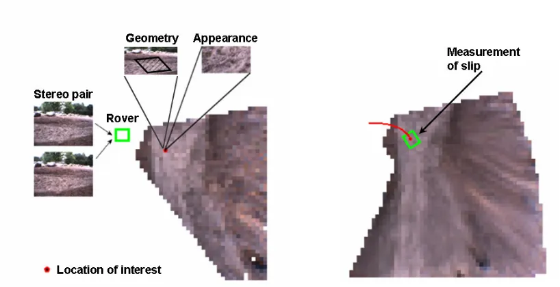
Our approach to this problem is to correlate the visual information and the cor-responding measured slip while the rover is traversing the terrain. In particular, we extract information about the terrain observed from a distance by using information from a stereo pair only, measure the slip of the rover when it traverses this particu-lar region, and create a mapping between visual information and the resultant slip (Figure 2.1). We propose to learn this functional relationship using the experience from previous traversals [4, 7, 9]. Thus, after learning, the expected slip can be pre-dicted from a distance using only stereo imagery as input. A learning approach is chosen, because 1) creating a physical slip model is extremely complicated due to the large number of variables involved; 2) the mapping from visual input to a mechanical terrain property, such as slip, is a complex function which does not have a known analytical form or a physical model, and one possible way to observe it and learn about it is via training examples; and 3) a learning approach promotes adaptability of the vehicle’s behavior.

To address the problem of slip learning and prediction we propose a general frame-work in which the task is subdivided into: 1) learning the terrain type from visual appearance and then, after the terrain type is known, 2) learning slip from the terrain geometry using nonlinear approximation. We term the latter dependence of slip on terrain geometry, when the terrain type is known, slip behavior. The proposed de-composition of the problem is adequate because from a mechanical point of view it is known that different terrains exhibit different slip behavior characteristics [15, 116], and because terrain appearance can be considered approximately independent of ter-rain geometry. This decomposition also introduces some structure in the problem, so that we can solve it with a reasonable amount of training data.

(30)

[image:30.612.114.523.74.284.2]

Figure 2.1: Main idea: Learning of slip output from visual information. The rover col-lects visual information (appearance and geometry) about a future location of interest in the forward-looking map from its stereo pair images (left). When this location is reached by the rover, a slip measurement is taken using onboard sensors (right). Cor-relating vision information to the corresponding slip measurement and learning this mapping allows for prediction of slip from a distance using visual information only.

This work is the first to attempt predicting slip from a distance. We have proposed an overall solution framework in which the slip is learned and predicted from visual information.

For the purposes of practical realization of the proposed method we also introduce a novel software architecture for navigation which can process data and predict slip in a more efficient way.

2.2 Definition of slip

Slip z is defined as the difference between the velocity measured by the wheel (wr) and the actual velocity v: z = wr−v, where w is angular wheel velocity and r is the wheel radius [130]. It can also be normalized by the commanded wheel velocity:

(31)

two consecutive stereo pairs) [54]. It can also be normalized, to receive a unitless slip value or express it in percentage of the step size. In this work we use the normalized version of slip for the whole rover.

For the kinematic estimate, we use the rover’s full kinematic model, which can be a simple differential drive model, a more complex rocker-bogie kinematic model [113, 54], or other model, as appropriate to the specific robot. The actual position (ground truth) can be estimated by visually tracking features [86, 88], a method called Visual Odometry (VO), or measured with some global position estimation device. VO is the preferred method for ground truth estimation because it is a convenient, self-contained sensor on the vehicle. By using VO, data collection and training can be done automatically, onboard the rover, which coincides with the goals of planetary ex-ploration missions. Furthermore, global positioning devices are not always available, especially in planetary missions.

Validation of VO position estimation has been performed by several groups [54, 93, 96]. VO position estimation error has been measured to be less than 2.5% of the distance traveled, compared to ground truth surveyed with a Total Station that has 2 mm precision, for runs of 20–30 meters in outdoor testing [54]. Similar results of 1.2% position error for a 20 m traverse have been achieved by [96] while testing in different circumstances, i.e., using a smaller robot, wide field of view cameras, different image resolution, etc. VO path length errors of about 1%–1.6% for 180–380 m traverses in outdoor environments have been reported by [93] with a different VO algorithm. The results of these tests indicate that VO is a precise position estimation technique and is adequate for use as ground truth both for computing slip per step and for precise localization within short to mid-size (20 m) traverses (i.e., to be able to map correctly the position of the location seen from a distance to the location traversed later on).

(32)

Although some vehicles have additional kinematically observable DOFs [113, 54], these three are the ones which matter most with regards to slip. Slip is normalized by the commanded velocity in X and will be expressed in percent. There will be cases in which the commanded forward velocity is 0, e.g., a purely crabbing motion of the rover, which will make the slip value undefined. As those cases are rare, we remove those steps from our dataset.

We have adopted a macro-level (of the whole rover) modeling of slip, in the spirit of [54, 81]. More specifically, our assumptions are that, between two consecutive steps, the rover will be traversing approximately locally planar and homogeneous regions, and the weight distribution on all its wheels will be the same. These assumptions mean that we consider slip (i.e., predict the terrain type, estimate terrain slopes, etc.) in regions comparable in size to the size of the robot or its wheel and not at the pixel level, for example. Naturally, those assumptions are violated in our field data, which is taken on real-life terrains with all complications, such as uneven and nonhomogeneous terrain, clumps on the ground, or rocks in front of the wheels. For example, when one of the wheels traverses a rock, an unexpected slip in Yaw might occur, because the rock creates different traction compared to the soil or can serve as an additional external force to the vehicle. As similar events are not modeled by our system, there will be some sources of sometimes significant noise in the slip measurements in our data. Nevertheless, this macro-level modeling is justified, as the slip prediction is intended to be used in a first, quick evaluation of terrain traversability to be handed down to a planner. More complex mechanical slip modeling can be applied [63, 65, 71], but to predict slip, information about soil mechanical properties of the forthcoming terrain is still required. These approaches deal better with uneven terrain, e.g., if dynamic simulation of the traverse over detailed terrain elevation models is performed [65], but they will be considerably more computationally expensive.

(33)

stepwise by the commanded velocity. Since Mars rovers are controlled with constant wheel velocity, only averaging of consecutive steps was needed.

2.3 Previous work

Although early work in autonomous navigation and traversability analysis based on forward looking sensors did not use learning [67, 45], learning-based approaches have started to become more and more preferred [19, 68, 87, 89, 98, 120, 127]. The reason is that intelligent autonomous behavior needs to be adaptive to the environment and the more complex the environment is, the less likely it is that predefined rules or heuristics will work well. This is particularly true for outdoor, off-road, unstructured environments which offer a lot of challenges (e.g., variability in terrains and lighting conditions, lack of structure, lack of prior information, etc.), and in which learning approaches have proved to be more appropriate [34, 58, 77, 80, 89, 106, 120, 127, 128]. Related work on vision-based perception of the forthcoming terrain has been con-sidered for the purposes of determining the mobility of Mars rovers [58], or the traversability in tall grass and foliage for off-road [73, 82] and agricultural vehi-cles [128], for detecting the drivable rural road in the context of off-road autonomous navigation [101], or for detecting obstacles in indoor [118] and outdoor environ-ments [13, 68].

Detecting or measuring rover slip occurring while driving can be achieved relatively easily by comparing the commanded velocity to the actual achieved velocity. An estimate of the actual velocity can be obtained from inertial measurements, GPS signals [22], or by visually tracking features, i.e., VO [54]. Alternative methods based on analyzing motor currents have also been used [95]. Providing an estimate of the possible slip at a location not yet traversed has not yet been attempted.

(34)

geometry. They are computationally intensive and impractical in the present setup. As slip depends also on the mechanical soil characteristics [15, 116], additional esti-mation of soil parameters, such as cohesion and friction angle [61, 76], or modeling of the soil behavior [2] needs to be done. Methods for online terrain parameter esti-mation [61], for recognizing terrain types [28], and for characterizing terrain traffica-bility [94] from onboard mechanical sensors have been proposed, but these estimates apply to the present vehicle location. No method, to our best knowledge, is available for predicting terrain parameters from a distance. One way to address this problem is by using forward looking sensors, e.g., vision, as proposed in this work.

Although slip has been acknowledged as an omnipresent problem in localization, especially in rough-terrain mobility [56], very few authors have considered counter-acting slip for improving vehicle mobility. Among them are the slip compensation algorithm of Helmick et al. [54, 55], in which the slip, measured at a particular step, is taken into account to adjust the next step, compensating for the distance which was not traversed; and the algorithm for improving traction control, proposed by Iagnemma et al. [60]. However, those methods, again, work at the traversed rover location and do not allow for planning at a distance, which our method enables.

Previous approaches have used manually created functions of slip as dependent on slopes [81]. Slip measurements were performed on short traverses of the rover on a tilt-table platform set to varying slope angles. These results showed that slip is a very nonlinear function of terrain slopes. For example, in deep sand, slip of about 20% on a 10◦ _{slope and of about 91% on a 20}◦ _{slope was measured, when}

the rover was driving straight upslope. The results of these experiments have been used successfully to teleoperate the Opportunity rover out of Eagle Crater, but the approach is very labor intensive, as it requires manual measurements. It also needs careful selection of the soil type on which the tests are performed to match the target Mars soil. Another limitation is that no slip models were available for angles of attack different from 0◦_{, 45}◦_{, or 90}◦ _{from the gradient of the terrain slope [29]. The}

(35)

model. We believe that learning slip is a more general approach, namely, the same learning algorithm can be applied to another vehicle to learn its particular behavior on different terrains. Moreover, the proposed method enables the vehicle to apply the learned models dependent on what it has sensed from the environment.

The work described above concerns estimating slip from mechanical measure-ments, or, in our case, visual information. Conversely, slip measurements have been used to infer mechanical terrain parameters on the Mars Pathfinder Mission in a controlled one-wheel soil-mechanics experiment [91]. Similar experiments have been done by [10] for MER. This gives us the assertion that slip characteristics are directly correlated to terrain mechanical properties and the intuition that if the terrain soil type could be correctly recognized (which would entail its mechanical properties) then slip behavior is predictable.

2.4 Experimental rover platforms

This research is targeted for planetary rovers, such as the Mars Exploration Rover (Figure 2.2, top left). For experimental purposes we tested our algorithm on two Mars research rover testbeds developed by NASA [104]: Rocky8 (Figure 2.2, top right) and Pluto (Figure 2.2, bottom left). We also used extensively the LAGR robot1 _{(Figure 2.2, right), as it is a more convenient data collection platform.}

Rocky8 is a prototype research rover with six wheels in a rocker-bogie configuration which allows for improved mobility on rough terrain [104]. It is one of the series of rovers created by NASA to develop and test technology for the MER mission. In the experiments presented, we have used its hazard detection stereo cameras with 80◦

horizontal field of view (FOV), its wheel encoders, rocker and bogie angle sensors, and IMU. Stereo pair imagery is acquired after each stop of the robot or in a continuous manner. The rover’s nominal speed of operation is 8 cm/s. Rocky8 is about 0.5 m tall.

1

(36)

[image:36.612.137.514.70.415.2]

Figure 2.2: Robot platforms. The Mars Exploration Rover Spirit in the JPL Space-craft Assembly Facility (top left). The Rocky8 rover in the Mojave desert (top right). The Pluto rover in the JPL Mars Yard (bottom left). The LAGR robot on off-road terrain (bottom right).

The Pluto rover (Programmable Logic Rover) is mechanically similar to Rocky8. The significant difference comes from its avionics which are based on a set of dis-tributed processors, or Programmable Logic Devices.2 _{Pluto has similar hazard}

cam-eras as Rocky8 (110◦ _{FOV). Additionally, a pair of color panoramic cameras (45}◦

FOV) are mounted on a ∼1.5 m tall mast with additional pan/tilt DOFs. The im-agery from the panoramic cameras will be used for slip prediction, whereas the hazard cameras are used for VO, which is in turn exploited to compute slip and provide ego-motion estimation.

The LAGR robot has two front differential drive wheels and two rear caster wheels. 2

(37)

[image:37.612.130.521.63.266.2]

Figure 2.3: Example images from some of the terrains collected by the LAGR vehi-cle: sand, soil, gravel, woodchips, asphalt. The ‘grass’ class will also appear in the sequences, although the rover has not driven on grass terrain in this dataset.

It is equipped with stereo cameras with 70◦ _{horizontal FOV, wheel encoders, IMU,}

and GPS. The robot can run in autonomous mode or be manually joysticked using a radio controller. It can achieve speeds of up to 1.2 m/s, although for some of our experiments it was set to drive at 30 cm/s. Stereo imagery is acquired continuously at 5 Hz. The LAGR robot is about 1 m tall.

2.5 Datasets

In this section we briefly describe the datasets collected and used in the experiments presented in this work.

2.5.1 Dataset collected by the LAGR robot

(38)

dry grass, which we considered as a single ‘grass’ class in the terrain classification in Section 2.8.

The terrains contain irregularities, undulations of the surface, small rocks, and grass clumps for off-road terrains or discolorations for asphalt. Although we have good variability in the terrain relief in our dataset (level, upslope, and downslope areas on soil, asphalt, and woodchip terrains; transverse slope on gravelly terrain; flat sandy terrain; etc.), not all possible slip behaviors could be observed in the area of data collection. For example, there was no sloped terrain covered with sand; besides, the LAGR robot showed poor mobility on flat sand, i.e., about 80% slip. The gravelly terrain available could only be traversed sideways for safety reasons; there was no transverse slope for the soil or asphalt datasets. We have collected a total of ∼5000 frames which are split approximately into 3000 for training and 2000 for testing. The distance covered by the rover during the data collection is roughly about 1 km. This data has been used extensively for testing in Sections 2.8, 2.9, and 2.10.

2.5.2 Datasets collected by the Mars prototype rovers

Several datasets have been collected with the Mars prototype rovers Rocky8 and Pluto in the Mojave desert and in the JPL Mars Yard.

One dataset was collected with the Rocky8 rover in the Mojave desert (Figure 2.5, left). It covers a distance of about 30 m. A single ‘sand’ terrain has been traversed in this dataset.

A second dataset was collected with Rocky8 in JPL’s Mars Yard (Figure 2.5, right). There are two terrain types present in this dataset: ‘Mars-like soil’ and ‘sand’. The terrain traversed consists of slopes of various inclinations. Since only two terrains are available, we have used this dataset primarily for evaluation of the slip prediction performance, rather than terrain recognition (Section 2.10.3).

(39)

[image:39.612.111.538.75.328.2]

Figure 2.4: Example patches from each of the classes in the dataset collected by LAGR: sand, soil, gravel, woodchips, asphalt, and grass. The best resolution patches (i.e. taken by the robot at 1–2 m range) are shown. The data are collected at different times of day/year, under various weather conditions. The variability in texture appearance is one of the challenges present in our application domain.

Figure 2.5: Rocky8 rover on sandy slopes in the Mojave desert (left) and in the JPL Mars Yard (right).

(40)

Figure 2.6: The Mars prototype rover Pluto in the JPL Mars Yard (left). An image showing the types of terrains available in this dataset (right).

rock’, is also present in the dataset. The rover did not drive over the rocks during the data collection, since they are obstacles, but it may still be desirable for them to be recognized and avoided.3 _{This dataset contained a variety of slopes as well.}

This setting is used for demonstrating the results of integrating the slip prediction algorithm on the rover in Section 2.11.

2.6 General framework for slip learning and

pre-diction

In this section we propose a general framework to learn the functional relationship between visual information and the measured slip using training examples.

The amount of slippage for a given vehicle depends on the soil type and the terrain’s geometry [15], so both geometry G, captured by the terrain’s slopes, and appearance A, e.g., texture and color, must be considered. At training time, the information about appearance and geometry coming from the stereo imagery is cor-related with the measured slip (in X, Y, or Yaw) as the robot traverses the cell. At query time, geometry and appearance alone are used to predict slip.

3

(41)

2.6.1 General framework

The dependence of slip on terrain slopes, called earlier slip behavior, is known to be highly nonlinear [81], but the precise relationship varies with the terrain type [15]. So, we cast the problem into a framework similar to the Mixture of Experts frame-work [64], in which the input space is partitioned into subregions, corresponding to different terrain types, and then several functions, corresponding to different slip be-haviors, are learned for each subregion. That is, in each region one model of slip behavior would be active, i.e., when the terrain type is known, slip will be a function of terrain geometry only.

More formally, let I be all the information available from stereo pair images,

I = (A, G). Let f(Z|I) =E(Z|I) be the regression function of slip Z (Z can be any of the slip in X, in Y, or in Yaw) on the input variables A, G (used interchangeably with the image information I). Now, considering that we have several options for a terrain type T, each one occurring with probability P(T|A, G), given the information from the image in question A, G, we can write f(Z|I) as follows:

f(Z|I) = f(Z|A, G) = X

T

P(T|A, G)f(Z|T, A, G), (2.1)

where PT P(T|A, G) = 1. This modeling admits one exclusive terrain type to be

selected per image, or a soft partitioning of the space, which allows for uncertainty in the terrain classification. We assume that the terrain type is independent of terrain geometry P(T|A, G) = P(T|A) and that, given the terrain type, slip is independent of appearancef(Z|T, A, G) = f(Z|T, G). Assuming independence of appearance and geometry is quite reasonable because, for example, a sandy terrain in front of the rover, will appear approximately the same, no matter if the rover is traversing a level or tilted surface. So we get:

f(Z|I) = X

T

P(T|A)f(Z|T, G). (2.2)

(42)

(P(T|A), i.e., the probability of a terrain type, given some appearance information) and a slip prediction part (f(Z|T, G), i.e., the dependence of slip on terrain geometry, given a fixed terrain typeT). For simplicity, instead of the mixing coefficientsP(T|A), we use a single winner-take-all terrain classification output:

T(A) = argmaxTP(T|A). (2.3)

However, using the probabilistic output P(T|A), if available, has more advantages. For example, it can implement smooth transitions between terrains and can provide confidence intervals for the final slip prediction.

The terrain classification output T(A) will be learned and predicted by a terrain classifier (Section 2.8). The regression functions fT(Z|G) = f(Z|T, G) for different

terrain typesT will be learned and predicted by a nonlinear regression method (Sec-tion 2.9). More precisely, suppose we are given training data D = {(xi,yi), zi}Ni=1,

where xi is the i-th appearance input vector, yi is the i-th geometry input vector,

zi is the corresponding slip measurement, and N is the number of training examples

(x,yare particular representations of the appearanceAand geometryGinformation in the image, respectively). We will independently train a texture classifier T(x) to determine the terrain type, using the appearance information x in Section 2.8 and a nonlinear function approximation ZT(y) = fT(Z|G = y) for a particular terrain

type T in Section 2.9. When doing testing we will use the full input vector (x,y), recognize the terrain type T0 = T(x), and then predict slip, as a function of slopes,

from the slip behavior function ZT0(y) learned for the terrainT0.

(43)

ex-ploited information about the structure of the problem, i.e., that the slip behavior can change depending on terrain [15]. The alternative to introducing structure in the problem is pooling appearance and geometry features, which will not only make the problem more complex because of increased dimensionality, but will also require a formidable amount of training data. This framework is general and, in principle, allows for different ways of addressing the problems of learning to recognize terrain types from appearance, and different algorithms for learning of slip behavior from terrain geometry.

2.6.2 Architecture

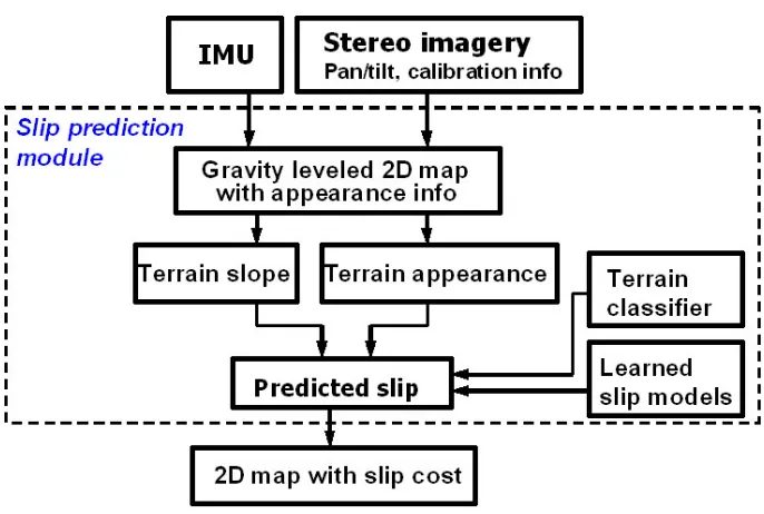
In this section we briefly describe the architecture of our system, summarized in Figure 2.7. We will be using the stereo imagery as input, as well as the IMU of the vehicle and its wheel encoders (the latter is needed only for training). Stereo imagery is used to create a 2D cell map of the environment from its range data. It also provides appearance information for each cell in the map. The 2D map contains geometry information about the terrain (G) and, as we are interested in terrain slopes with respect to gravity, we use the vehicle’s IMU to retrieve an initial gravity-leveled pose. In fact, a filtered IMU signal is used, often in conjunction with other onboard sensors. The appearance information from color imagery (A) will be used to decide which terrain type corresponds to a cell or a neighborhood of cells. This is all the information necessary to perform slip prediction with our algorithm. The advantage of such a system is that it can sense the terrain remotely and that it needs only passive, cheap, and self-contained sensors on the vehicle, such as stereo vision.

(44)

[image:44.612.152.495.66.297.2]

Figure 2.7: Slip prediction algorithm framework.

sensors, is needed for a rocker-bogie type of vehicle, such as Rocky8, Pluto, or MER, but it is well understood how to compute it [113, 54]. Differencing the actual motion and the motion estimated by the kinematic model gives a measurement of slip for a particular step. This feedback is used for collecting training examples to learn slip from stereo imagery.

2.7 Software architecture

In this section we describe the software architecture of the slip prediction algorithm, which is designed to provide efficient processing of the data from the surrounding terrain. Since processing of visual features is generally time consuming, the focus has been on decreasing the amount of computations devoted to terrain classification. The utilization of the slip prediction algorithm as a part of a larger autonomous navigation system [53] is also taken into consideration. Namely, it is expected that the following constraints need to be satisfied:

(45)

man-ner. For example, a set of images might be received first, e.g., when taking a panorama, and only after that is any query for slip cost at an arbitrary location of the terrain invoked.

—Redundant data input. A typical scenario will obtain multiple, partly over-lapping images of the terrain, i.e., a map cell may obtain information from multiple images. It is also possible that slip-related cost would not be needed for some areas of the map, e.g., in areas where obstacles have already been detected.

— Memory and computational efficiency. Although there are no specific restrictions regarding memory usage and computational time at the research and development stage, these two important aspects have to be taken into consideration in view of real-time testing onboard the rover.

The software architecture is novel and is designed to accommodate the require-ments described above. In particular, our main concern is evaluating the terrain type per map cell, rather than evaluating the terrain type in the whole image. More specif-ically, we create a map cell structure which contains a set of pointers to images which have observed the cell and the corresponding rover pose (viewpoint) from which it has been observed (Figure 2.8). In this way, the map cells can invoke the terrain classification mechanism only if, or when, needed. A ring buffer of images which have been recently acquired is also supported. The images can be accessed multiple times for terrain classification purposes. Note also that it provides efficient storage of information. That is, no additional patches, texture signatures, etc., need to be stored explicitly.

This idea is in contrast to standard systems for autonomous navigation [19, 49], which are based on processing the whole area of each acquired image and updating the map with the corresponding information. We call this architecture patch-centered as opposed to the pixel-centered processing of previous autonomous navigation systems. Note that the proposed method does not compromise the performance of the sys-tem, it is just a more efficient way of processing, storing, and accessing the available information.

(46)

Figure 2.8: Schematic of the software design paradigm: each map cell keeps a set of pointers to images which have observed it. An image patch, corresponding to a map cell, is retrieved and processed once, e.g., when terrain classification or slip prediction needs to be done, thus avoiding redundant computations.

cell works as follows: a projection of the map cell to the image is done and an image patch corresponding to this cell is retrieved. In this way when multiple images observe a map cell, we can retrieve the image patch corresponding to the map cell which contains most information about the map cell. In this case not all image patches need to be processed, which avoids redundant computations, but at the same time allows for obtaining of multiple decisions about a map cell, if needed. Figure 2.9 shows an example in which nine images cover the whole terrain, but by using the proposed method, we can effectively process the data corresponding to three images only (less processing is required in the cases when some of the map cells do not need to be evaluated).

The main assumption made is that the regions in which slip prediction is needed are relatively planar. An example when this assumption is violated is a portion of the terrain which contains large rocks. In this case the projected terrain patch of a map cell near a large rock might contain portions of the rock because of occlusions. However, in our case this assumption will be satisfied since the slip prediction is intended to be used after processing the terrain for geometric obstacles, e.g., large rocks (see Section 2.11). That is, there is no need to predict slip in areas which are known to be non-traversable due to obstacles.

(47)

[image:47.612.182.466.68.277.2]

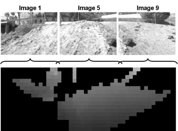
Figure 2.9: Example of full coverage of the map by only a third of the images ob-tained. The software architecture allows for more efficient processing of the data. For example, the elevation map shown has been built from nine panorama images, but effectively the visual information from only three images need to be processed to fully classify the terrain.

identical images, or if it does not receive imagery, etc. In either of the cases, the map is updated with new information, if such is available, and whenever a terrain classification is invoked, only the most recent terrain patch is used. The result of the terrain classification is saved with its corresponding confidence and might be combined with a potentially new evaluation if the confidence is insufficient. This is in contrast to processing fully all of the incoming images, extracting visual features and saving them to the map cells.

(48)

close range cover large portions of the image, compared to map cells at far ranges, this can speed up the processing without hurting the overall performance. This will be taken advantage of later in Chapter 5 when a variable-length terrain representation is proposed. We further discuss the slip prediction module software architecture in the context of running it as a part of an integrated autonomous navigation system in Section 2.11.

2.8 Terrain classification

This section describes terrain classification (T(A)) using vision information, which is the first step of our algorithm. For the purposes of slip prediction, we consider only the part of the image plane which corresponds to the robot’s 2D map of the environment. That is, for now, we are not interested in regions beyond the distance where range data is available, because we simply cannot retrieve any reliable slope information and therefore cannot predict slip. A reasonable map for the LAGR vehicle is of size 12x12 m or 15x15 m, centered on the vehicle. Note that the MER panoramic camera has considerably higher resolution and look-ahead [18]. The map is subdivided into cells, each one of size 0.4x0.4 m. Our goal is to determine the terrain type in each cell of the map. In fact, we will be classifying the patches corresponding to the projections of map cells to the image plane.

(49)

[image:49.612.126.516.74.326.2]

Figure 2.10: Schematic of the terrain classification algorithm [79, 123].

the horizon [89]. So, for our experiments we build five independent classifiers which are active at different ranges (ranges up to 2 m, 2–3 m, 3–4 m, 4–5 m, and 5 m and above).

2.8.1 Terrain classification algorithm

As we are interested in classifying patches, corresponding to map cells, the approach we use considers the common occurrence of texture elements, called ‘textons’, in a patch. This representation is appropriate, because a texture is defined not by a single pixel neighborhood, but rather by the co-occurrence of visual patterns in larger regions. The idea follows the texton-based texture recognition methods proposed by [79, 121, 123]. The approach is summarized in Figure 2.10.

(50)

a local pixel neighborhood. Those vectors are clustered with k-means and the cluster centers are defined to be the textons for this class. We extracted k=30 textons per class.4 _{As a result, a total of 180 textons, called ‘texton dictionary,’ are collected for}

the whole training set. Working in a feature space composed of local neighborhoods allows for building statistics of dependencies among neighboring pixels, which is a very viable approach, as shown by [123].

Now that the dictionary for the dataset has been defined, each texture patch is represented as the frequencies of occurrences of each texton within it, i.e., a his-togram.5 _{In other words, the patches from the training set are transformed into}

180-dimensional vectors, each dimension giving the frequency of occurrence of the corresponding texton in this patch. All vectors are stored in a database to be used later for classification. Similarly, during classification, a query image is transformed into a 180-dimensional vector (i.e., a texton occurrence histogram) and compared to the histogram representations of the examples in the database, using a Nearest Neighbor method and a χ2_{-based distance measure [123]. The majority vote of N=7}

neighbors is taken as the predicted terrain class of the query patch. The result of the classifier will be one single class. To determine the terrain type in the region the robot will traverse (Section 2.10) we select the winner-take-all patch class label in the cell neighborhood region. In both decisions, a probabilistic response, rather than choosing a single class, would be more robust.

2.8.2 Terrain classification results

In this section we report results of the terrain classification algorithm on data col-lected by the LAGR robot (Section 2.5.1). Our dataset is composed of five different image sequences which are called soil, sand, gravel, asphalt, and woodchip after the prevailing terrain type in them (Figure 2.3), but an additional ‘grass’ class can appear in those sequences. As mentioned earlier, we consider patches in the original color

4

As seen in the experiments later in the thesis, the number of textons can vary in a certain range without affecting the final performance significantly.

5

(51)

image that correspond to cells of the map. Each patch is classified into a particular terrain type and all the pixels which belong to this patch are labeled with the label of the patch (Figure 2.11). To measure the test performance we take ∼30 frames in each sequence, which are separated by at least 10 frames within the sequence, so as not to consider images similar to one another. The test set contains a total of ∼150 frames which span ∼1500 frames. The ground truth terrain type in the test set is given by a human operator. Example classification results are shown in Figure 2.11. Summary results of the terrain classifier for the five sequences for different look-ahead distances are given in Figure 2.12. Classification performance is measured as the percent of correctly classified area (i.e., number of pixels) in the image plane and the correctly classified patches corresponding to cells in the map. The drop-off in performance, especially in terms of patches, is due to a large number of classification errors at far range. This is expected, as the patches at far range correspond to very small image area (with little information content) and therefore are much more likely to be misclassified. Naturally, regarding slip prediction, a larger map is preferred, as it allows the robot to see farther, but the terrain classification errors at far ranges can make slip prediction unreliable at large distances. Therefore, a tradeoff between accuracy of classification and being able to see farther must be made. To be concrete, in our further experiments we fix the map size at 12x12 m. The confusion matrix6 _for

the terrain classification for the 12x12 m map, when considering correctly classified pixels, is shown in Figure 2.12. From it we can see that grass is often misclassified as woodchips (this happens for the areas of dry grass (Figure 2.11, top left)), soil is sometimes misclassified as sand and vice versa, asphalt is misclassified as gravel, etc.

2.8.3 Discussion

The texton-based algorithm has been previously applied to artificial images [123], but not to the autonomous navigation domain. Our main motivation for using it here

6

(52)

Sand Soil Grass

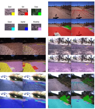
[image:52.612.137.516.67.504.2]

Gravel Asphalt Woodchip

Figure 2.11: Example texture classification results from each of the datasets. Patches from the six terrain types considered in the texture classification, and the correspond-ing color codcorrespond-ing assigned are shown at top left. Each composite image contains the original image (top left), the ground truth terrain classification (bottom left) and the results of the terrain classification algorithm represented in two different ways (top right and bottom right). Ambiguous terrain type in the ground truth is marked with white. Those regions are not required to be classified correctly.

is that slip prediction requires fine discrimination between visually similar terrains, such as soil, sand, and gravel. The texton-based approach is also robust to intra-class variability, often observed in natural terrains.

(53)

6x6m 10x10m 12x12m 15x15m 18x18m 20 40 60 80 100

Classification rate (%)

Map size

Terrain classification summary

Pixels Patches 0.77 0.74 0.74 0.33 0.84 0.85 True class Predicted class

Terrain classification rate=76.4%

sand soil grass gravel asph. wchip wchip asph. gravel grass soil sand

Figure 2.12: Terrain classification results for different map sizes (left). Different ways of representing the classification rate by counting correctly classified patches or pixels are shown. Confusion matrix for the 12x12 m map (right). The classification rate for each class is displayed on the diagonal.

which is patch-oriented, i.e., the classification of the terrain is done per image patch, corresponding to a map cell. The usage of the proposed architecture provides for the texture algorithm to be range dependent, i.e., to apply different classifiers for patches at different ranges. The architecture also allows taking advantage of faster classifi-cation methods, if such are available, and classifying some portion of the map cells more efficiently, thus decreasing the overall computational time. Such an algorithm is proposed in Chapter 5.

2.9 Learning slip behavior on a fixed terrain

In this section we describe the method for learning to predict slip as a function of terrain geometry, when the terrain type is known, i.e., the slip behavior.

Visual Prediction of Rover Slip: Learning Algorithms and Field Experiments