Appraisal Framework for Integrated Transport

This is a repository copy of Appraisal Framework for Integrated Transport. White Rose Research Online URL for this paper:

http://eprints.whiterose.ac.uk/2516/

Monograph:

Shires, J.D. and Johnson, D. (2003) Appraisal Framework for Integrated Transport. Working Paper. Institute of Transport Studies, University of Leeds , Leeds, UK. Working Paper 578

eprints@whiterose.ac.uk https://eprints.whiterose.ac.uk/ Reuse

See Attached

Takedown

If you consider content in White Rose Research Online to be in breach of UK law, please notify us by

White Rose Research Online

http://eprints.whiterose.ac.uk/

Institute of Transport Studies

University of Leeds

This is an ITS Working Paper produced and published by the University of Leeds. ITS Working Papers are intended to provide information and encourage discussion on a topic in advance of formal publication. They represent only the views of the authors, and do not necessarily reflect the views or approval of the sponsors.

White Rose Repository URL for this paper: http://eprints.whiterose.ac.uk/2516/

Published paper

Shires, J.D. and Johnson, D. (2003) Appraisal Framework for Integrated

Working Paper 578

September 2003

Appraisal Framework for Integrated Transport

Authors

J.D. Shires and D. Johnson

UNIVERSITY OF LEEDS

Institute for Transport Studies

ITS Working Paper 578

September 2003

Appraisal Framework for Integrated Transport

J.D. Shires and D. Johnson

Contents Page

Section Page Number

1. Introduction 3

2. Key Implications From the Integrated Transport Project 3

3. The Appraisal Framework 4

3.1 The GOMMMS Framework Outlined 4 3.2 An Adapted GOMMMS Framework 5

3.2.1 Environment 6

3.2.2 Modal Shift & The Economy 7

4. Data Requirements and Calculations Outlined 8

4.1 Drivers 8

4.1.1 The Demand Model & Forecasting Passenger Trips 8 4.1.2 Diversion Factors, Vehicle Kilometres and Passenger Trips 12

4.2 Factors 13

4.2.1 The Environment 13

4.2.2 Modal Shift and The Economy 15

4.2.3 Private Transport Providers 16

4.2.3 Government Impacts 17

4.3 Summary 17

5. Appraisal Results & Conclusions 18

5.1 General Comments on the UK Average Appraisal Values 26 5.2 General Comments on the Non-Average UK Appraisal Values 26

5.3 Conclusions 26

References: 27

ACKNOWLEDGEMENTS

1 Introduction

This working paper outlines an appraisal framework for the Integrated Transport project. The project examined the demand implications from the introduction of a Taktfahrplan timetable onto the east coast mainline rail route. The Taktfahrplan concept is frequently referred to as an interval timetable and is based on trains leaving stations at the same time past the hour throughout the operational day. A stated preference exercise was conducted to estimated what values people placed on such a timetable and these values were added to the more conventional elements of generalised cost to obtain the changes in demand that would result from the introduction of a Taktfahrplan.

The working paper is divided into a number of sections that will highlight,

• the key implications to arise from the Integrated Transport project;

• the demand model;

• the appraisal framework;

• the data sources used within the appraisal framework; and

• the results of the appraisal framework.

Interested readers are also referred to the a conference paper that will be presented at the European Transport Conference in Strasbourg later this year (Wardman et al, 2003).

2 Key Implications from the Integrated Transport

Project

The key aim of the Integrated Transport project has been to redesign the current rail network timetable around a Taktfahrplan system. The key attribute of a Taktfahrplan system is that trains depart from a station at the same time past the hour every hour of the operational day. Achieving such a design has involved the,

• Closing of certain rail stations;

• Removal of some rail services; and the,

• Streamlining of some rail services in terms of frequency and the stations they serve.

There are obviously a number of implications stemming from this that include,

1) How does it affect existing rail passengers?

• will the generalised cost of rail travel fall or increase?

• will they switch to other modes or continue to use rail;

2) How will it affect non-rail passengers?

• will they be attracted to rail;

• will they be affected by higher levels of road congestion?

3) How will other public transport operators be affected

• will their revenues be reduced or increased;

• will services increase or decrease;

• will operating costs change;

• what levels or road congestion will they face;

• will there be journey time increases or decreases?

4) How will the government be affected?

• will rail subsidies increase or decrease?

5) How will this impact on externalities?

• Local air quality;

• Greenhouse gases;

• Noise; and

• Safety.

6) What will be the social consequences in terms of social exclusion and distributional impacts?

In order to appraise these implications we will need to ensure that we have the correct information to calculate the likely impacts and the correct appraisal framework to present them. In the next section the appraisal framework is presented.

3

The Appraisal Framework

3.1 The GOMMMS Framework Outlined

The appraisal framework that has been developed is largely based upon the GOMMMs (Guidance on the Methodology for Multi-Modal Studies) appraisal framework which are used by the Highways Agency for appraising new road building/enhancement projects.

The GOMMMS framework attempts to examine the impacts of transport proposals in terms of the impact such proposals have on all modes of travel. The main objective of a GOMMMS assessment is to examine the strategic implications of a scheme and it therefore tends to concentrate on objectives that are relevant to Central Government as opposed to Local Government.

“

• integration – ensuring that all decisions are taken in the context of our integrated transport policy;

• safety – to improve safety for all road users;

• economy – supporting sustainable economic activity in appropriate locations and getting good value for money;

• environmental impact – protecting the built and natural environment; and

• accessibility – improving access to everyday facilities for those without a car and reducing community severance.”

The results of the GOMMMS appraisal are presented in an Appraisal Summary Table. This is a one page table that summarises the impacts of a scheme and provides decision makers with a clear and transparent basis to make judgements. The AST presents a range of impact data in various forms, namely, financial (transport economic efficiency), quantitative (tonnes of CO2) and qualitative (landscape).

3.2 An Adapting GOMMMS Framework

The GOMMMS assessment framework provides a clear and concise presentation of the financial and social costs and benefits. As such it makes an idea blueprint framework for the Integrated Transport project. However, a full GOMMMS appraisal is not required for this project and we have instead produced a framework that focuses on just the key indicators and presents them as an AST (Table 3.1).

Table 3.1 Integrated Transport AST

Appraisal Summary Sheet Enhancement Route Type Measurement Period Modes Considered Date: 11/08/03 Timetable A Intercity Weekly Rail and Car

Objective Quantitative Impacts Financial Costs/Benefits Low High 1. The Environment

1.1 Noise

1.2 Local Air Quality 1.3 Greenhouse Gases 1.4 Safety

Total

2. Modal Shift & The Economy

2.1 User Benefits

Rail Users Gen. Cost

Car Users Congestion

Bus Users Congestion

2.2 Private Transport Providers Revenues Costs Profits

2.3 Government Indirect Tax Rail Subsidy

Total CBA Measure

3.2.1 Environment

a) Noise

Noise levels vary by traffic levels, type of traffic, speed of traffic, road type, time of day, existing noise levels and the type of environment the traffic is located in. The latter factor is what drives the different values as that will determine how many people (residents, workers, shoppers etc...) are affected by changes in noise levels, e.g. additional traffic on a rural motorway will have a negligible impact on the population, whilst additional traffic on an urban motorway will have a significant impact on the population.

b) Local Air Quality

Local air quality (LAQ) can have significant health impacts upon those people exposed to them. The most significant emissions are PM10 and NO2 which can be particularly high in urban areas and very problematic when combined with poor atmospheric dispersion. Again the key factor is the number of people experiencing a change in pollution levels

c) Greenhouse Gases

The Kyoto summit recognised six greenhouse gases but singled out carbon dioxide emissions (CO2) as the most important greenhouse gas. This makes it the most important indicator of global warming. It can be calculated directly from changes in fuel consumption using emission factors providing in DMRB and is measured in tonnes.

d) Accidents

Accidents result in a number of impacts that affect both individuals (casualties and non-casualties) and organisations. The impacts are outlined below:

• medical and healthcare costs;

• lost economic output;

• pain and suffering;

• material damage;

• emergency services costs;

• insurance administration; and,

• legal and court costs.

3.2.2 Modal Shift & The Economy

a) Modal Shift

Modal shift impacts upon a number of impacts within the Integrated Appraisal AST and these are listed below.

• change in time and money costs to users existing and generated;

• change in operating costs and revenues;

• change in externalities;

• change in road user costs; and,

• change in accident costs.

Modal shift can see passenger switch between all the transport modes, all of which need to be taken into account.

b) Economy

Rather than present a single measure of economic worth the Integrated Transport AST breaks the results of the appraisal into a number of components parts in order to highlight the different impacts on different groups. The components parts are listed below and are discussed in turn:

• Users;

• Private sector transport providers; and,

• Other Government impacts.

1. Users

User benefits in this case are calculated for rail passengers as changes in generalised cost, with the rule of the half applied in each case. The key components of the generalised cost include,

• Changes in travel attributes – wait time, IVT etc; and,

• Changes in user charges – fares.

For car and coach travellers the changes in user benefits take the form of changes in congestion costs and the rule of a half is not applied.

2. Impacts on Private Transport Providers

3. Calculation of Other Government Impacts

The indicators used to measure other government impacts are changes in indirect tax revenue (fuel duties and VAT on fuel) and grants/subsidies (to train operating companies).

With the appraisal framework outlined the next section now concentrate on how the impacts can be calculated and the data inputs required for those calculations.

4 Data

Requirements

and

Calculations Outlined

The general data requirements for calculating the impacts outlined in the appraisal framework fall into two categories,

• Drivers – changes in vehicle kilometres (all modes and road type), changes in trips (all modes) and diversion factors (all modes).

• Factors – factors which are applied to the drivers to calculate the value of the impacts – emission values per vehicle kilometre (vkms), accident values per vkms , congestion values per vkms, fare values per vkms, generalised cost values per vkms and indirect tax values etc.

In the next two sub-sections we discuss the drivers and the factors respectively.

4.1 Drivers

The key driver for the whole appraisal is the change in passenger trips that is forecast as a direct result of the introduction of the new Taktfahrplan timetable. The

modelling process is described below and was based upon a model developed by Lythgoe (Lythgoe, 2003). The modelling takes into account the changes between the base timetable and the new Taktfahrplan timetable and also the values attached to Taktfahrplan attributes such as roundnumberedness (ie memorability) and

clockfaceness.

4.1.1 The Demand Model & Forecasting Passenger Trips

In order to carry out an evaluation of the benefits of Taktfahrplan we needed to generate forecasts of the changes in demand and revenues for Origin Destination (OD) pairs on a selected part of the network. The case study chosen was the East Coast Mainline.

In order to generate the forecasts required for our case study, the forecaster requires:

• A list of OD pairs specifying the flows for which forecasted volumes will be generated

• A set of Generalised Journey Times (GJTs) containing one for each OD pair

• A set of TAKT indices, 8 for each OD pair (although in the final calibration of the model only two of these were used).

If new sets of GJTs and TAKT indices for a selected OD pair are not specified, the forecasts are based on default values used in the calibration of the Lythgoe model. In this way the forecaster can generate the ‘base’ ie, ‘as now’, predicted volumes for selected OD pairs.

In our East Coast Mainline case study, the introduction of the Taktfahrplan produces a new timetable which generates changes in GJTs and TAKT indices. The new values of GJTs and TAKT associated with the new ‘Tyler’ timetable are then used to generate forecasts of predicted demand between each of the significant OD pairs on the ECML network. The base and predicted forecasts generated form the basis of the subsequent evaluation exercise.

The following sections describe the data preparation required in order to generate these forecasts of changes in demand for flows on the East Coast Mainline following the introduction of Taktfahrplan.

Selection of Stations and Flows for Calibration:

The Lythgoe model is based flows greater than 461 per year, ie the top 10%. This cut-off point yields 12,253 flows. From these flows, we had information on 438 stations.

In order to incorporate TAKT indices into the Lythgoe model, we needed the complete set of opportunities to travel (OTTs) for the existing timetable. This was provided by the AEAT. AEAT provided data on OTTs between 178,727 OD pairs based on 538 stations. The common set of stations between the Lythgoe dataand the AEAT data was 358

The list of common OD pairs is then used to filter out the relevant OTTs for calibration from the AEAT timetable data. This yields 10,324 flows for which there are OTTs (and thus, potentially TAKT indices) and that feature in the Lythgoe dataset. These were the flows used for the calibration of the model.

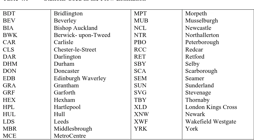
East Coast Main Line Case Study:

Table 4.1 Stations Used in the Flow Estimation BDT BEV BIA BWK CAR CLS DAR DHM DON EDB GRA GRF HEX HPL HUL LDS MBR MCE Bridlington Beverley Bishop Auckland Berwick- upon-Tweed Carlisle Chester-le-Street Darlington Durham Doncaster Edinburgh Waverley Grantham Garforth Hexham Hartlepool Hull Leeds Middlesbrough MetroCentre MPT MUB NCL NTR PBO RCC RET SBY SCA SEM SUN SVG TBY XLD XNW XWF YRK Morpeth Musselburgh Newcastle Northallerton Peterborough Redcar Retford Selby Scarborough Seamer Sunderland Stevenage Thornaby

London Kings Cross Newark

Wakefield Westgate York

Of these, Garforth (GRF), Musselburgh (MUB), Seamer (SEM), and Thornaby (TBY) did not appear in the MOIRA list of stations used by the Lythgoe model. Flows based on these stations could not be forecasted.

Calculation of GJTs:

In order to generate GJTs from the new ‘Tyler timetable’, Viriato was used to scope the new timetable, and then MOIRA converted the stopping patterns generated from the new timetable into journey opportunities and GJTs.

1009 instances of GJTs were derived, based on flows where changes the OTTs set should be ‘complete and real’. However, they were in the form of GJTs for full, reduced and in some cases, season individual ticket types. Also, because the MOIRA GJTs were averaged over the two directions, they only appeared for one direction.

The 1009 GJTs supplied were found to correspond to 858 flows. Of these, 124 did not appear in the Lythgoe dataset.

An average GJT weighted by the share of each ticket type for each flow was calculated, and specified in two directions, so that they could be used as inputs into the forecasting tool.

Bearing in mind the volumes are different for a pair of flows in opposite directions, although the ticket specific GJTs will be the same, the weighted average is likely to be different for the two directions.

The forecasting program was checked against predicted values from the Lythgoe model and it was found to replicate the same results, given the same data inputs. However, because of the irreconcilable difference in GJTs between those used in the Lythgoe model and those generated from the runs of MOIRA based on the existing timetable, we decided that in order for consistency between the GJTs used in the base and those used in the forecasting we would estimate the base using the MOIRA GJTs.

However, because the Lythgoe model is based on competition between stations, some of the competitor origin stations do not appear in the ECML study. In these cases we retain the GJTs used in the calibration of the Lythgoe model.

TAKT information for the existing timetable:

The 10,324 flows are then selected from the AEAT dataset and used as inputs into the ‘autotakt’ program written by Peter Wightman. This program creates values for a variety of TAKT indices for each of the flows. These TAKT measures included various indices capturing the degree of clockfaceness of services’ departure and arrival times, measures of ‘evenintervalness’, and ‘roundnumberedness’ of a service.

After various sensitivity tests, we found that continuous versions (ie not simply 0/1 dummies based on a threshold level), of the 0,5,10 minute roundnumberedness (ie memorability) and the departure clockfaceness indices were the most significant determinants of demand, so were included in the variables for the calibration of the model. These two indices could also be used in conjunction with values from the stated preference study carried out for this project, which gave values to clockfaceness and memorability in terms of minutes, which could then be included in the calculation of generalised cost.

Takt indices for the new timetable:

As described above, TAKT indices were calculated for the existing timetable, based on the OTTs provided for us by AEAT. However, given the use of the memorability, or round numberedness index, as an explanatory variable in the calibrated Lythgoe model, we also had to generate these indices for the new timetable.

In order to calculate the new TAKT indices, a new set of OTTs needed to be generated. This was a two stage process:

Firstly, with reference to the net graph and the MOIRA input files, details of each service, including stopping stations, and arrival and departure times, were keyed in two excel spreadsheets.

Secondly, these excel files were used as input files to a program which generated a stopping patterns file for all these services based on a representative eight hour

sample of departure times reducing run-times. This generates a ‘stopping patterns’ file.

‘PRAISE’ contains a module, again written by Peter Wightman, which constructs OTTs based on stopping patterns, so, after 2.5 days of processing time, a new set of OTTs were created for the new timetable for ECML. These OTTs were fed into ‘autotakt’ as before and TAKT indices of the same form as for the original timetable were created.

As was the case for GJTs, for non-ECML flows, new TAKT data would be missing, so we used the TAKT indices from the base, eg in the case of Wakefield to York, Sheffield is a competitor station to Wakefield, but no TAKT information is available from the MOIRA input files.

4.1.2 Diversion Factors, Vehicle Kilometres and Passenger Trips

Diversion Factors & Passenger Trips:

The change in rail passenger trips can be used to calculate the modal shift between rail, car, coach and not travel or new journeys. An integral part of these calculations are the application of diversion factors to the change in passenger trips. For example, if the number of rail trips are assumed to have increased by 10,000 per year, diversion factors can be used to ascertain where those journeys have come from. In the appraisal the following diversion factors (Table 4.1) were used to estimate the sources of new rail journeys and vice versa (see Table 4.1).

Table 4.1 Diversion Factors & Sources of New Rail Journeys

Diversion Factors % Sources of New Rail Journeys %

Car 68% Car 6,800

Bus 24% Bus 2,400

New 8% New 800

From the table it is clear that 6,800 of the the 10,000 new rail journeys are being made by people who used to travel by car; that 2,400 trips are made by former coach passengers; and, that 800 journeys are new in that they weren’t made previous to the introduction of the new timetable. This information can be taken forward and used to calculate a number of the impacts outlined in the appraisal framework.

Diversion Factors & Vehicle Kilometres:

Table 4.2 Calculating Modal Switch in Terms of Journeys

Modal Switch

(journey)Calculations

Modal Switch (journeys)

Car 6,800/1.6 4,250

Bus 2,400/12.1 198

To calculate the total number of car and coach vehicle kms that has been switched the total distance of the trip needs to be factored in. For out appraisal this process has been taken a step further and the total distance has been disaggregated into three road types,

• Motorways;

• Trunk and Principal Roads; and,

• Other Roads

If it is assumed that all the journeys relate to one flow between Leeds and London then the modal switch in relation to car and coach vehicle kms can be calculated using the following disaggregated distances,

• Motorways – 301.44 kms

• Trunk and Principle Roads – 18.18 kms

• Other Roads – 0 kms

These figures then need to be factored by the number of journeys for each mode to calculate the total modal switch in terms of vehicle kms.

Table 4.3 Total Modal Switch – In Terms Vehicle Kms

Mode Total Number of Journeys

Total Motorways Vkms

Total Trunk & Principle Vkms

Total Other Vkms

Total Vkms

Car 4,250 1,281,120 77,265 0 1,358.385

Bus 198 59,685 3,600 0 63,285

Totals 4,448 1,340,805 80,865 0 1,421,670

This information can be taken forward and used to calculate a number of the impacts outlined in the appraisal framework.

4.2 Factors

In this section we outline the factors used in the calculation of the impacts listed in Table 3.1 and the methodologies employed to calculate them.

4.2.1 The Environment

area types, 3 road types, 5 vehicle types and 2 time periods. For rail the disaggregation is by passenger service type (3 categories). We present two sets of figures for each type of environmental impact. The first set outline National UK average values which do not disaggregate to any detail. The second set disaggregates values by type of road and peak and off peak.

The UK average values for environmental factors are presented in Table 4.4, whilst the disaggregated values are presented in Tables 4.5 and 4.6

Table 4.4 UK Average Values of Environmental Factors (£s in 1998 Prices and Values)

Impact Type Bus Car

Noise 0.0009 0.0001

LAQ 0.0316 0.0018

Greenhouse Gases 0.0056 0.0012

Safety 0.0374 0.0079

Table 4.5 Disaggregated Values of Environmental Factors (£s in 1998 Prices and Values)

Impact Type – BUS Peak Off Peak Combined

Rural Motorways:

Noise 0.0001 0.0001 0.0001

LAQ 0.0076 0.0076 0.0076

Greenhouse Gases 0.0042 0.0042 0.0042

Safety 0.0119 0.0119 0.0119

Trunk & Principal:

Noise 0.0015 0.0015 0.002

LAQ 0.0392 0.0392 0.039

Greenhouse Gases – from London

0.0065 0.0059 0.006

Greenhouse Gases – to London - - 0.006

Greenhouse Gases - Regional - - 0.006

Safety 0.0042 0.0042 0.004

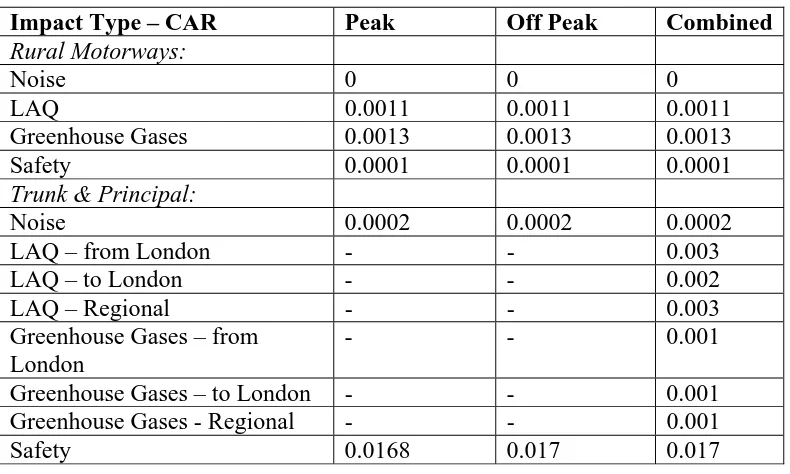
Table 4.6 Disaggregated Values of Environmental Factors (£s in 1998 Prices and Values)

Impact Type – CAR Peak Off Peak Combined

Rural Motorways:

Noise 0 0 0

LAQ 0.0011 0.0011 0.0011

Greenhouse Gases 0.0013 0.0013 0.0013

Safety 0.0001 0.0001 0.0001

Trunk & Principal:

Noise 0.0002 0.0002 0.0002

LAQ – from London - - 0.003

LAQ – to London - - 0.002

LAQ – Regional - - 0.003

Greenhouse Gases – from London

- - 0.001

Greenhouse Gases – to London - - 0.001

Greenhouse Gases - Regional - - 0.001

Safety 0.0168 0.017 0.017

When presenting the change in environmental costs in the appraisal table, the car and coach impacts are added together.

4.2.2 Modal Shift and the Economy

User Benefits

For rail the change in user benefits can be reflected in the change in the generalised costs to existing users of the rail service following the change in the timetable. The model outlined in 4.1.1 calculates the change in generalised cost and this has been subjected to the rule of a half to obtain the change in user benefits for rail users.

For car and coach travellers the change in user benefits is reflected by the change in congestion costs that they incur. The costs of congestion are outlined in Tables 4.7 for average UK values and in Tables 4.8 and 4.9 for disaggregated values. The key values are the combined values which are used in the appraisal. In most cases the values for the peak and off-peak are the same. When this isn’t the case we have had to calculate three values to reflect the peak and off-peak splits of train journeys that are coming from London, are going to London or that are regional in nature.

Table 4.7 UK Average Values of Congestion (£s in 1998 Prices and Values)

Impact Type Bus Car

Table 4.8 Disaggregated Values of Congestion (£s in 1998 Prices and Values)

Impact Type – BUS Peak Off Peak Combined

Rural Motorways:

Congestion – from London - - 0.0626

Congestion – to London - - 0.0619

Congestion – Regional - - 0.0624

Trunk & Principal:

Congestion – from London - - 0.208

Congestion – to London - - 0.192

Congestion - Regional - - 0.205

Table 4.9 Disaggregated Values of Noise (£s in 1998 Prices and Values)

Impact Type – CAR Peak Off Peak Combined

Rural Motorways:

Congestion – from London - - 0.004

Congestion – to London - - 0.004

Congestion – Regional - - 0.004

Trunk & Principal:

Congestion – from London - - 0.139

Congestion – to London - - 0.128

Congestion - Regional - - 0.137

4.2.3 Private Transport Providers

We have assumed that the number of rail services has not changed following the introduction of the new rail timetable. Rails costs are therefore assumed to have remained constant Coach services on the other hand are assumed to have fallen and the following cost factors per vehicle kilometre are assumed (Sansom et al, 2001)

• Motorway – 19 pence

• Trunk & Principal – 10 pence

• Other – 10 pence.

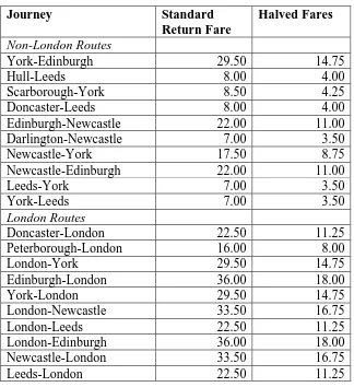
Table 4.10 National Express Standard Fares (£s – 2003)

Journey Standard Return Fare

Halved Fares

Non-London Routes

York-Edinburgh 29.50 14.75

Hull-Leeds 8.00 4.00

Scarborough-York 8.50 4.25

Doncaster-Leeds 8.00 4.00

Edinburgh-Newcastle 22.00 11.00

Darlington-Newcastle 7.00 3.50

Newcastle-York 17.50 8.75

Newcastle-Edinburgh 22.00 11.00

Leeds-York 7.00 3.50

York-Leeds 7.00 3.50

London Routes

Doncaster-London 22.50 11.25

Peterborough-London 16.00 8.00

London-York 29.50 14.75

Edinburgh-London 36.00 18.00

York-London 29.50 14.75

London-Newcastle 33.50 16.75

London-Leeds 22.50 11.25

London-Edinburgh 36.00 18.00

Newcastle-London 33.50 16.75

Leeds-London 22.50 11.25

4.2.3 Government Impacts

The impact of indirect tax directly affects government revenues. For cars the government levies fuel duty and VAT on fuel duty. For coaches it is the VAT not paid that has to be calculated. Values per average UK vehicle kms have been taken from the Sansom et al (2001) publication and are presented in Tables 4.

Table 4.11 UK Average Values for Indirect Taxes Per Vehicle Kms (£s-1998)

Mode Fuel Duty VAT on Fuel Duty VAT Not Paid

Car 0.0386 0.0068 na

Bus na na 0.1278

With regards to subsidy we have assumed that rail vehicle kilometres remain constant and so there will not be any affect on subsidy payments.

4.3 Summary

5)

Appraisal Results & Conclusions

In this section the results of the appraisals are outlined. The full model estimated the change in flows from a change in the East Coast mainline route timetable. For the purposes of this exercise it was felt appropriate that only a selection of flows should be analysed. As such only the top 10 London and non-London flows (ranked according to passenger flows) are examined. The routes selected are outlined in Table 4.12.

Table 5.1 Routes Selected for Appraisal

Non-London Routes Ranking

York-Edinburgh 10 Hull-Leeds 9 Scarborough-York 8 Doncaster-Leeds 7 Edinburgh-Newcastle 6 Darlington-Newcastle 5 Newcastle-York 4 Newcastle-Edinburgh 3 Leeds-York 2 York-Leeds 1

London Routes Ranking

Doncaster-London 10 Peterborough-London 9 London-York 8 Edinburgh-London 7 York-London 6 London-Newcastle 5 London-Leeds 4 London-Edinburgh 3 Newcastle-London 2 Leeds-London 1

Table 5.2 Appraisal Results for Non-London Flows – Using Average UK Values

Impact York-Edinburgh

Hull -Leeds Scarborough

-York Doncaster-Leeds Edinburgh-Newcastle Darlington-Newcastle Newcastle-York Newcastle-Edinburgh Leeds-York York-Leeds

Change in Rail Passenger Trips -1,870 17,221 12,440 21,724 12,432 23,953 16,501 20,221 70,518 76,992

1. The Environment

1.1 Noise

1.2 LAQ

1.3 Greenhouse Gases Safety -35 -803 -356 -2,352 99 2,295 1,019 6,724 50 1,147 509 3,360 65 1,511 671 4,426 127 2,928 1,300 8,578 83 1,918 851 5,620 143 3,302 1,465 9,673 207 4,791 2,126 14,035 186 4,303 1,910 12,605 203 4,698 2,085 13,763

Total -3,545 10,136 5,066 6,673 12,923 8,472 14,583 21,159 19,004 20,748

2. Modal Shift & The Economy

2.1 User Benefits Rail – GC Car – Congestion Bus – Congestion

2.2 Private Transport Providers Rail Revenues Rail Costs Rail Profits Coach Revenue Coach Costs Coach Profits 2.3 Government Indirect Tax Rail Subsidy 53,552 -21,815 -1,760 -21,1961 0 52,026 6,701 -8,537 -1,836 11,029 0 70,583 62,371 5,032 52,026 0 52,026 -16,739 24,407 7,668 -31,533 0 30,581 31,171 2,515 27,188 0 27,188 -12,848 12,198 -650 -15,759 0 77,550 41,060 3,313 35,725 0 35,725 -21,116 16,.068 -5,048 -20,758 0 66,005 79,571 6,420 93,183 0 93,183 -33,230 31,138 -2,092 -40,228 0 82,538 52,132 4,206 44,397 0 44,397 -20,372 20,401 29 -26,357 0 84,627 89,729 7,240 68,271 0 68,271 -35,085 35,113 28 -45,364 0 152,889 130,193 10,504 136,989 0 136,989 -54,051 50,948 -3,103 -65,822 0 127,243 116,933 9,434 128,625 0 128,625 -59,976 45,758 -14,218 -59,118 0 160,912 127,668 10,300 137,315 0 137,315 -65,482 49,959 -15,523 -64,545 0

Total 17,208 166,147 75,047 131,841 202,858 156,946 204,532 361,650 308,900 356,129

Table 5.3 Appraisal Results for London Flows – Using Average UK Values Impact Doncaster-London Peterborough -London London-York Edinburgh-London York-London London-Newcastle London-Leeds London-Edinburgh Newcastle-London Leeds-London

Change in Rail Passenger Trips 34,794 101,844 -3,592 -29,874 -5,370 -13,923 55,319 -49,096 -4,456 72,463

1. The Environment

1.4 Noise

1.5 LAQ

1.6 Greenhouse Gases Safety 588 13,598 6,035 39,837 859 19,877 8,822 58,233 -71 -1,647 -731 -4,825 -1,201 -27,778 -12,329 -81,380 -106 -2,462 -1,093 -7,214 -377 -8,727 -3,874 -25,568 1,065 24,647 10,939 72,207 -1,972 -45,610 -20,244 -133,622 -121 -2,793 -1,240 -8,183 1,964 45,420 20,160 133,066

Total 60,058 87,792 -7,274 -122,687 -10,876 -38,546 108,859 -201,447 -12,336 200,609

2. Modal Shift & The Economy

2.1 User Benefits Rail – GC Car – Congestion Bus – Congestion

2.2 Private Transport Providers Rail Revenues Rail Costs Rail Profits Coach Revenue Coach Costs Coach Profits 2.3 Government Indirect Tax Rail Subsidy 240,701 369,548 29,816 501,840 0 501,840 -95,119 144,612 49,493 -186,832 0 306,009 540,200 43,584 722,481 0 722,481 -197,985 211,393 13,954 -273,108 0 -38,278 -44,758 -3,611 -57,657 0 -57,657 12,873 -17,515 -4,642 22,628 0 -344,714 -754,920 -60,908 -428,037 0 -428,037 130,669 -295,417 -164,748 381,663 0 130,474 -66,921 -5,399 -89,676 0 -89,676 19,247 -26,188 -6,941 33,833 0 -176,462 -237,182 -19,136 -229,772 0 -229,772 56,672 -92,815 -36,143 119,912 0 601,335 669,831 54,043 967,465 0 967,465 -151,227 262,120 110,893 -338,645 0 -713,542 -1,239,542 -100,008 -738,700 0 -738,700 214,746 -485,061 -270,315 626,673 0 84,419 -75,906 -6,124 -67,180 0 -67,180 18,137 -29,704 -11,567 38,376 0 594,429 1,234,388 99,593 1,177,272 0 1,177,272 -198,096 483,044 284,948 -624,067 0

Total 1,004,567 1,352,575 -126,317 -1,371,663 -4,630 -578,784 2,064,921 -2,435,434 -37,983 2,766,563

Table 5.4 Appraisal Results for Non-London Flows - Using Non-Average UK Values

Impact York-Edinburgh

Hull -Leeds Scarborough

-York Doncaster-Leeds Edinburgh-Newcastle Darlington-Newcastle Newcastle-York Newcastle-Edinburgh Leeds-York York-Leeds

Change in Rail Passenger Trips -1,870 17,221 12,440 21,724 12,432 23,953 16,501 20,221 70,518 76,992

1. The Environment

1.7 Noise

1.8 LAQ

1.9 Greenhouse Gases Safety -66 -1,062 -376 -4,130 45 1,475 1,050 3042 94 1,518 538 5,901 52 1,209 695 3,339 240 3,874 1,373 15,063 54 1,402 880 3,495 185 3,433 1,532 11,736 393 6,339 2,246 24,647 344 5,595 2,015 21,587 376 6,109 2,200 23,569

Total -5,634 5,611 8,050 5,295 20,551 5,831 16,886 33,625 29,542 32,255

2. Modal Shift & The Economy

2.1 User Benefits Rail – GC Car – Congestion Bus – Congestion

2.2 Private Transport Providers Rail Revenues Rail Costs Rail Profits Coach Revenue Coach Costs Coach Profits 2.3 Government Indirect Tax Rail Subsidy 53,552 -33,281 -2,376 -21,961 0 -21,961 6,701 -8,537 -1,836 11,029 0 70,583 23,785 3,139 52,026 0 52,026 -16,739 24,407 7,668 -31,533 0 30,581 47,553 3,395 27,188 0 27,188 -12,848 12,198 -650 -15,759 0 77,550 26,541 2,624 35,725 0 35,725 -21,116 16,068 -5,048 -20,758 0 66,005 121,391 8,666 93,183 0 93,183 -33,230 31,138 -2,092 -40,228 0 82,538 27,636 3,021 44,397 0 44,397 -20,372 20,401 29 -26,357 0 84,627 94,140 7,584 68,271 0 68,271 -35,085 35,113 28 -45,364 0 152,889 198,619 14,179 136,989 0 136,989 -54,051 50,948 -3,103 -65,822 0 127,243 173,919 12,506 128,625 0 128,625 -59,976 45,758 -14,218 -59,118 0 160,912 189,886 13,654 137,315 0 137,315 -65,482 49,959 -15,523 -64,545 0

Total 5,127 125,668 92,309 116,633 246,923 131,264 209,287 433,749 368,958 421,700

Table 5.5 Appraisal Results for London Flows – Using Non-Average UK Values Impact Doncaster-London Peterborough -London London-York Edinburgh-London York-London London-Newcastle London-Leeds London-Edinburgh Newcastle-London Leeds-London

Change in Rail Passenger Trips 34,794 101,844 -3,592 -29,874 -5,370 -13,923 55,319 -49,096 -4,456 72,463

1. The Environment

1.10Noise

1.11LAQ

1.12Greenhouse Gases Safety 113 7,040 6,190 8,492 1,015 19,560 9,204 64,432 -111 -1,914 -768 -6,983 -356 -15,734 -12,668 -24,941 -166 -2,861 -1,148 -10,441 -511 -9,303 -4,053 -32,303 149 12,138 11,209 11,901 -581 -2,5804 -20,799 -40,777 -229 -3,696 -1,309 -14,370 2,660 48,416 21,096 168,115

Total 21,835 94,211 -9,775 -53,698 -14,616 -46,170 35,397 -87,961 -19,604 240,286

2. Modal Shift & The Economy

2.1 User Benefits Rail – GC Car – Congestion Bus – Congestion

2.2 Private Transport Providers Rail Revenues Rail Costs Rail Profits Coach Revenue Coach Costs Coach Profits 2.3 Government Indirect Tax Rail Subsidy 240,701 63,350 14,628 501,840 0 501,840 -95,119 144,612 49,493 -186,832 0 306,009 516,103 43,063 722,481 0 722,481 -197,985 211,393 13,408 -273,108 0 -38,278 -56,152 -4,253 -57,657 0 -57,657 12,873 -17,515 -4,642 22,628 0 -344,714 -191,228 -33,048 -428,037 0 -428,037 130,669 -295,417 -164,748 381,663 0 130,474 -83,958 -6,360 -89,676 0 -89,676 19,247 -26,188 -6,941 33,833 0 -176,462 -259,272 -20,580 -229,772 0 -229,772 56,672 -92,815 -36,143 119,912 0 601,335 86,402 25,060 967,465 0 967,465 -151,227 262,120 110,893 -338,645 0 -713,542 -312,568 -54,190 -738,700 0 -738,700 214,746 -485,061 -270,315 626,673 0 84,419 -115,800 -8,267 -67,180 0 -67,180 18,137 -29,704 -11,567 38,376 0 594,429 1,349,350 107,106 1,177,272 0 1,177,272 -198,096 483,044 284,948 -624,067 0

Total 683,181 1,327,957 -138,354 -780,111 -22,627 -602,317 1,452,510 -1,462,642 -80,019 2,889,038

5.1 General Comments on the UK Average Value Appraisal Values

It is interesting to note that in terms of the change in rail passenger trips the move towards a Taktfahrplan timetable appears to very beneficial for non-London flows (9 of the 10 routes experience an increase in passenger trips) and non-beneficial for London flows (6 of the 10 routes experience a reduction in passenger trips). This may reflect the more variability of current regional flows and that the Taktfahrplan timetable tends to reduce the number of services for certain London based flows compared with current levels. In particular the long distance London based flows seem to be particularly adversely affected (Edinburgh and Newcastle) compared to those under 200 miles (Leeds, Doncaster and Peterborough).

The impact of environmental benefits tends to be overshadowed by the impacts arising from modal shift and the economy. There also seems to be a disproportionate affect from coach costs compared with coach revenue. This may reflect the assumption used for calculating the change in coach vehicle kilometres.

Changes in rail revenue and car congestion also have an influential role in the appraisal, especially for the London based flows where fares are higher and journeys longer.

5.2 General Comments on the Non-Average UK Values

The use of non-average UK values tends to have different impacts upon the London and non-London flows. For the London flows the use of non-average UK values produces final appraisal values that are lower 70% of the time in comparison to when average UK values are used.. For non-London flows the figure is more balanced with 40% of the flows producing lower values.

The areas of difference are in the environment sub-impact and the change in user benefits.

5.3 Conclusions

References:

DETR (1998) “A New Deal for Transport”.

DMRB (2003) Volume 13, Highways Economics Note 1.

Lythgoe (2003) – To Insert

Sansom, T., Nash, C., Mackie, P., Shires, J.D. and Watkiss, P. (2001) “Surface Transport Costs and Charges: Great Britain 1998”. A Report for the DETR.