Recognizing trace graphs of closed braids

Fiedler, T. and Kurlin, V. Osaka J. Math.

47 (2010), 885–909

RECOGNIZING TRACE GRAPHS OF CLOSED BRAIDS

THOMAS FIEDLER and VITALIY KURLIN

(Received October 24, 2008, revised May 18, 2009)

Abstract

To a closed braid in a solid torus we associate a trace graph in a thickened torus in such a way that closed braids are isotopic if and only if their trace graphs can be related by trihedral and tetrahedral moves. For closed braids with a fixed number of strands, we recognize trace graphs up to isotopy and trihedral moves in polynomial time with respect to the braid length.

1. Introduction

1.1. Motivation and summary. There is still no efficient solution to the conju-gacy problem for braid groups Bn on n 5 strands, i.e. with a polynomial complexity

in the braid length. Very promising steps towards a polynomial solution were made by Birman, Gebhardt, González-Meneses [2, 3, 4] and Ko, Lee [13]. A clear obstruction is that the number of different conjugacy classes of braids grows exponentially even in

B3, see Murasugi [14].

The conjugacy problem for braids is equivalent to the isotopy classification of closed braids in a solid torus. To a closed braid in a solid torus we associate a 1-parameter family of closed braids, which is encoded by the labelled trace graph in a thickened torus. We call this construction a 1-parameter approach to links.

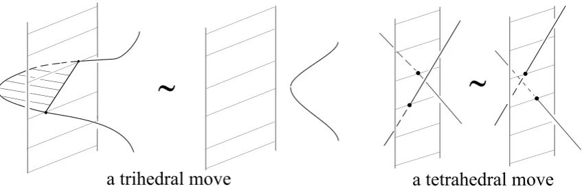
We establish the higher order Reidemeister theorem for closed braids: trace graphs determine families of isotopic closed braids if and only if they can be related by a fi-nite sequence of the trihedral and tetrahedral moves shown in Fig. 5 and Fig. 6, see Theorem 1.4. We recognize trace graphs of closed braids up to isotopy in a thickened torus and trihedral moves in polynomial time with respect to the braid length, see The-orem 1.5. This is one of very few known polynomial algorithms recognizing complicated topological objects up to isotopy.

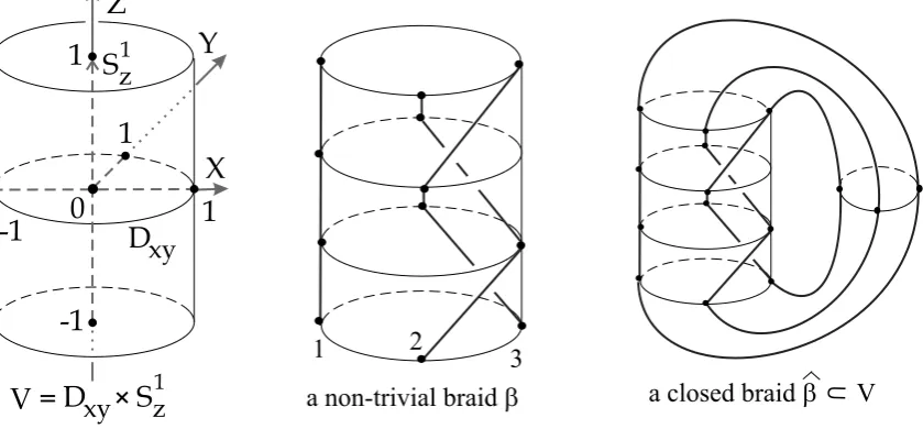
1.2. Basic definitions of braid theory. We work in the C -smooth category. To explain important constructions we may draw piecewise linear pictures that can be easily smoothed. Fix Euclidean coordinates x, y, z in 3. Denote by Dx y the unit disk

at the origin 0 of the horizontal plane XY. Introduce the solid torus V Dx y Sz1,

where the oriented circle S1

z is the segment [ 1, 1]z with the identified endpoints, see

the left picture of Fig. 1.

2000 Mathematics Subject Classification. 57M25.

Fig. 1. A braid and its closure in the solid torus V.

DEFINITION 1.1. Mark n points p1, , pn Dx y. A braid on n strands is

the image of a smooth embedding of n segments into Dx y [ 1, 1]z such that

• the strands of are monotonic with respect to pr_z S1

z (see Fig. 1);

• _{the lower and upper endpoints of are (pi 1 ), (pi 1 ), respectively.}

Identifying the bases Dx y z 1 , the cylinder Dx y [ 1, 1]z is converted into the

solid torus V Dx y Sz1, while a braid Dx y [ 1, 1]z becomes the closed braid

V, see the right picture of Fig. 1.

DEFINITION 1.2. Braids are considered up to an isotopy, a smooth deformation of the cylinder Dx y [ 1, 1]z, fixed on its boundary. The equivalence classes of braids

form the group denoted by Bn. The product of braids 1, 2 is the braid 1 2 obtained

by attaching a cylinder containing 2 over a cylinder containing 1. The trivial braid

consists of n vertical straight segments n_{i 1}(pi [ 1, 1]z).

The braid group Bn is generated by elementary braids i, i 1, ,n 1, where i is a right half-twist of strands i,i 1, the remaining strands are vertical. The braid

in the middle picture of Fig. 1 is isotopic to ₂2. Any braid induces a permutation of its endpoints, e.g. the braid induces the trivial permutation on 1, 2, 3. Such a braid

Bn is called pure and its closure consists of n components.

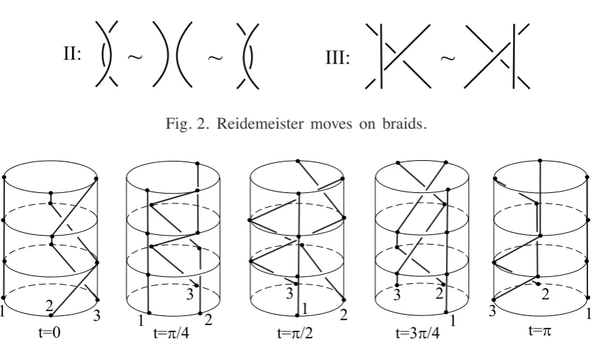
Fig. 2. Reidemeister moves on braids.

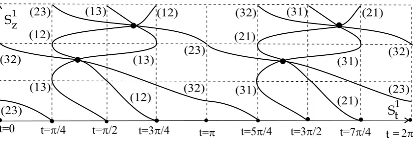
Fig. 3. Diagrams of rotated braids rott( ) for the braid in Fig. 1.

braids rotated around the core of the solid torus V. This family contains more combi-natorial information about a closed braid than just one plane diagram and involves such features of braids as meridional trisecants, straight lines meeting a braid in 3 points and contained in a meridional disk Dx y z of the solid torus V.

A long knot in 3_{, a single curve approaching the vertical axis Z at , can be}

also rotated in 3 _{around Z, but closed braids are more naturally rotated in V. It is}

essential to work in the solid torus instead of 3 since our 1-parameter family repre-sents a non-trivial rational homology class in the space of all diagrams. A. Hatcher has proven that the space of diagrams of a prime knot in 3 has a finite fundamental group [12]. Consequently, its rational first homology group vanishes.

DEFINITION 1.3. Given a closed braid V in a general position (see more

details in Subsection 2.1), consider rotated braids rott( ) V obtained by the rotation

of through an angle t [0, 2 ). Project each of the rotated braids rott( ) to the fixed

annulus Ax z [ 1, 1]x Sz1 V, see Fig. 3. The crossings of the resulting diagrams

form the trace graph TG( ) that lives in the thickened torus Ax z St1, see Fig. 4,

where the time circle S_t1 is [0, 2 ] with the identified endpoints.

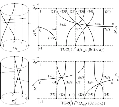
For the braid from Fig. 1, a triple point occurs in a diagram of rott( ), t

( 4, 2), where strand 1 crosses over strand 3, which crosses over strand 2. The associated vertex of TG( ) and its image under t t are in Fig. 4.

Label arcs of a pure braid Bn by 1, 2, ,n as in the middle picture of Fig. 1.

Fig. 4. The trace graph of the closed braid in Fig. 1.

diagram of a rotated braid rott( ), i.e. the point p evolves in following a trace of

crossings in the diagrams. Label the point p by the ordered pair (i j) if the arc i is over the arc j in the diagram of rott( ) and by the ordered pair (ji) otherwise. For

non-pure braids, other well-defined markings will be introduced in Definition 3.2. The trace graph maps to itself under the time shift t t , each label (i j) reverses to (ji). Each labelled closed loop of TG( ) is monotonic with respect to the vertical circle S1

z,

but not with respect to the time circle S1

t .

The trace graph of the piecewise linear closed braid in Fig. 1 is projected to the torus ZT Sz1 St1 and is shown in Fig. 4. A vertical section TG( ) (Ax z t )

of a trace graph consists of finitely many points, which are crossings of the diagram of rott( ), e.g. the zero section TG( ) (Ax z 0 ) contains 2 points associated to

the crossings of the original braid . The section TG( ) (Ax z 4 ) has 2 tangent

vertices, when the rotated braid rot 4( ) has 2 simple tangencies (arc 1 over arcs 2, 3),

so the diagram of rot 4( ) changes under Reidemeister moves II.

The braid has two meridional trisecants associated to two triplevertices of TG( ). Under the rotation of through some t ( 4, 2) and t ( 2, 3 4), the trisecants become perpendicular to the plane of projection, so triple intersections appear in the cor-responding diagrams of rott( ). Around these singular moments the diagrams change

under Reidemeister moves III, notice that the labels don’t change at triple points, see more details about singularities and general position of braids in Subsection 2.1. A given closed braid can be reconstructed from its trace graph with labels, see also combinatorial constructions of a trace graph in Subsection 2.2.

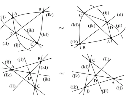
Theorem 1.4. Closed braids 0, 1 are isotopic in the solid torus V if and only

if their labelled trace graphs TG( 0), TG( 1) can be obtained from each other by

an isotopy in and a finite sequence of moves in Fig. 5 and Fig. 6.

inter-Fig. 5. Trihedral move on trace graphs.

sections !❅, i.e. under the rotation 3 crossings approach each other as in Reidemeister move III, but then go back in the reverse direction without completing Reidemeister move III. The tetrahedral move is associated to passing through the singular subspace of quadruple intersections ✦❛☞☞▲▲ , when a 1-skeleton of some tetrahedron collapses in the trace graph to a point and then blows up again in a symmetric form.

Theorem 1.4 can be used to construct invariants of closed braids reflecting such geometric features as meridional trisecants. Similar easily computable lower bounds on the number of fiber quadrisecants in knot isotopies were found by Fiedler and Kurlin [8]. On the other hand trace graphs turned out to be complicated topological objects that can be recognized up to isotopy in a polynomial time.

Theorem 1.5. Let , Bn be braids of length l. There is an algorithm of

complexity C(n 2)n2 8(6l)n2 n 1 to decide whether TG( ) and TG( ) are related by isotopy in and trihedral moves, the constant C does not depend on l and n. In the case of pure braids, the power n2 8 can be replaced by 1. If the closure of a braid is a knot, a single circle in the solid torus, then the complexity reduces to Cn(6l)n 1.

2. Studying closed braids in terms of their trace graphs

2.1. Singularities and general position of closed braids. Here we outline of the proof of Theorem 1.4, which follows from a more general result by Fiedler and Kurlin [9, Theorem 1.4] on links in the solid torus V.

Codimension 1 singularities of closed braids with respect to the plane projection are tangencies of order 1 ☎_✆✞_✝and triple intersections !❅ associated to Reidemeister moves II and III, respectively, see Fig. 2. The Reidemeister theorem says that any isotopy in the space SB of all closed braids (with respect to the Whitney topology) can be approxi-mated by a path transversal to the singular subspace ☎

✆ ✞

✝ !❅ SB. We extend this

approach to 1-parameter families of rotated closed braids.

Codimension 2 singularities of plane diagrams of closed braids are quadruple points

☞☞ ✦_▲▲

❛_{, tangent triple points} ✟☎ ✆ ✞

✝ and tangencies of order 2 ✆✞. A closed braid V can

be put in a general position such that the canonical loop of rotated braids rott( )

SB is transversal to the codimension 1 subspace ☎ ✆ ✞

✝ !❅ SB and avoids the

co-dimension 2 subspace ✦❛_☞☞▲▲ ✟☎ ✆ ✞

✝ ✆✞ SB. Similarly any isotopy of closed braids

can be approximated by a path s ss 10 such that the cylinder of canonical loops rott( s)

is transversal to ✦❛_☞☞▲▲ ✟☎ ✆ ✞

✝ ✆✞ SB. Passing through these singularities leads to

tetrahedral moves in Fig. 6, trihedral move in Fig. 5 and a move where a triple vertex!❅%

Fig. 7. A trihedral move and a tetrahedral move for braids.

first move in Fig. 6 applies when the intermediate oriented arcs go together from one side of the band to another like . The second move in Fig. 6 means that the arcs are antiparallel as in the British rail mark .

2.2. Combinatorial constructions of a trace graph. First we show how to cre-ate the trace graph using an algebraic form of a braid.

Lemma 2.1. Let Bn be a braid of length l. Then the closure is isotopic in

the solid torus V to a closed braid whose trace graph contains 2l(n 2) triple vertices.

Proof. Let Bn be Garside’s element [10], i.e. 2 is a generator of the center

of Bn, the full twist of n strands. The rotation of a braid Bn can be considered as

a commutation of with 2_{. So the canonical loop of rotated closed braids rot}

t( ) is

represented by the sequence of the closures of the following braids:

1 1 1 1 1 1 _.

The first arrow in the sequence consists of Reidemester moves II creating couples of symmetric crossings. The second arrow represents an isotopy of the diagram when we push through the trivial part of the closed braid , i.e. we cyclically shift the letters of 1 _{to get} 1 _{. The third arrow shows how acts on from the}

right. After we get a new braid , we apply the same transformation and finish with

since implies that .

For n 3, we have 1 2 1. We need to consider only the two generators 1, 2 and their inverses. We apply braid relations corresponding to Reidemeister moves II

and III associated to tangent and triple vertices of TG( ).

1 1( 1 2 1) 1( 2 1 2) 2,

2 2( 1 2 1) ( 1 2 1) 1 1, 1

1 11( 1 2 1) 2 1 ( 1 11) 2 1 1( 2 1 21) 21, 1

Fig. 8. Half trace graphs of the 4-braids 1, 21 B4.

Notice that the sequence is canonical in the case of a generator and almost ca-nonical in the case of an inverse generator. Indeed we can replace the above sequence

by 1

1 21 by 1 1( 1 2 1) 2 1 2 1( 2 21) ( 1 2 1) 21. Pushing

through a generator or its inverse creates exactly n 2 triple points. So we end up with 2l(n 2) triple points, because we push twice through the braid.

Now we construct a trace graph of a closed braid in a geometric way.

Lemma 2.2. Let Bn be a braid of length l. Then the closure is isotopic

in the solid torus V to a closed braid whose trace graph consists of elementary blocks associated to the generators (and their inverses) of Bn similar to Fig. 8.

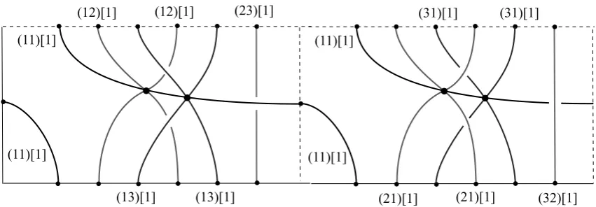
Proof. Fig. 8 shows the trace graphs of the elements 1 and 21 in the braid

group B4. In general we mark out the points k 21 k , k 0, , n 1 on the

The crucial feature of the distribution k is that all straight lines passing through

two points j, k are not parallel to each other. Firstly we draw all strands in the

cylinder Dx y [ 1, 1]z. Secondly we approximate with the first derivative the strands

forming a crossing by smooth arcs, see the left hand side pictures of Fig. 8.

Then each elementary braid i constructed as above has exactly n 2 meridional

trisecants, one trisecant through the strands i, i 1 and j for each j i,i 1. Each trisecant is associated to a triple vertex of the trace graph, see 4 meridional trisecants in the left hand side pictures of Fig. 8. The right hand side pictures in Fig. 8 contain the trace graphs of the corresponding 4-braids. The braids are not in general position, e.g. parallel strands 3 and 4 lead to the vertical arc labelled with (34), but we may slightly deform such a braid, which makes the projection TG S1

t generic.

3. Two splittings of trace graphs of closed braids

3.1. A trace graph splits into trace circles.

Lemma 3.1. For a braid Bn, let (n1, ,nm) be the lengths of cycles in the

induced permutation Sn. Number all components of the closure by 1, ,m. Set

N( ) m_{i 1}(ni 1) 2 i j gcd(ni,nj), gcd is the greatest common divisor.

(a) The trace graph TG( ) splits into N( ) circles such that each circle is a trace of crossings formed by 2 points simultaneously travelling along .

(b) If the braid is pure, i.e. the permutation is trivial, then N( ) n(n 1). If the closure of the braid is a knot, then N( ) n 1.

For any braid Bn, we have n 1 N( ) n(n 1).

Proof. (a) Denote by p1, , pn the intersections of with Dx y 1 , ordered

by the orientation of . Suppose that pr, ps belong to the q-th component of . This

component corresponds to a cycle of the length nq of the permutation Sn.

If we push pr, ps along their strands in , the associated point in TG( ) goes

along a circle and comes to the point corresponding to the next pair (say) (pr 1, ps 1).

This process continues until we come to the original pair (pr, ps) after nq steps along

the cycle of having passed through nq of nq(nq 1) ordered pairs. For each cycle

of length nq of Sn, we get nq 1 circles that can be distinguished by non-zero

differences r s (mod nq) 1, , nq 1 .

Assume that pr, ps are in different components i j of , associated to cycles

of lengths ni,nj. Then the process above terminates after lcm(ni,nj) steps, lcm is the

lowest common multiple, since at each step indices r,s shift by 1 in two sets of lengths ni,nj. For any two cycles of lengths ni,nj in , we get 2 gcd(ni,nj) circles split into

pairs symmetric with respect to the time shift t t .

Fig. 9. Trace circles in TG( 1) for the non-pure 4-braid 1 B4.

estimate N( ) n(n 1) geometrically follows from the fact that all circles from (a) are monotonic in the direction S1

z and each meridional disk Dx y z intersects in

exactly n points leading to n(n 1) crossings appearing under the rotation.

Let n1 be minimal among all lengths ni 1. Under the map (n1,n2, , nm)

(

n1

1, , 1,n2, , nm), the number N( ) of circles from (a) increases by

n1(n1 1) 2n1(m 1) (n1 1) 2

m

i 2

gcd(n1, ni)

(n1 1)2 2n1(m 1) 2

m

i 2

n1 (n1 1)2 0.

So N( ) is minimal if is a knot and maximal if is pure.

DEFINITION 3.2. For a braid Bn, a trace circle of the trace graph TG( )

is a circle consisting of crossings formed by 2 points simultaneously travelling along , e.g. a trace circle does not change its direction at triple vertices, compare Figs. 8 and 9. By Lemma 3.1 trace circles can be denoted by T(i j)[k] as follows. In the case

i j the trace circles T(ii)[k] are associated to crossings formed by the points of (Dx y

z ) from the i-th component of . If we index these points by 1, ,ni according

to the orientation of the i-th component then the number k 1, ,ni 1 in the

notation (ii)[k] is well-defined as the difference between the indices modulo ni. The

trace circles T(i j)[k] with i j are generated by the i-th and j-th components of .

Then k 1, , gcd(ni, nj) is defined up to cyclic permutation, i.e. if a trace circle

is marked by 1, this defines markings on other circles T(i j)[k], T(ji)[k], k 1.

EXAMPLE 3.3. Fig. 8 contains halfs of the trace graphs TG( 1), TG( ₂1) of the

Fig. 10. Markings of crossings and trace circles.

3, 4 of the strands in the 4-braids. Fig. 9 shows the complete trace graph TG( 1) split

into trace circles with markings (i j)[k] from Definition 3.2. The closure of 1 B4 has

m 3 components, the lengths of cycles in the permutation 1 S4 are (n1,n2, n3)

(2, 1, 1), hence TG( 1) splits into N( 1) 7 trace circles by Lemma 3.1 (a). One of

these 7 trace circles is marked by (11)[1] and is formed by self-crossings of the first component consisting of strands 1, 2. The remaining 6 trace circles are marked by (i j)[1] and are formed by crossings of different components, i.e.i, j 1, 2, 3 , i j. Trace graphs of some pure braids are in Fig. 11.

If is pure then the markings reduce to ordered pairs (i j), see Fig. 10. If the closure is a knot, the markings [k] have well-defined numbers k 1, , n 1 .

Lemma 3.4. Let Bn be a braid. Consider trace circles T(qr)[i],T(qs)[j],T(r s)[m]

passing through a triple vertex TG( ).

(a) The trace circle T(qs)[j] passes between T(qr)[i] and T(r s)[m] at the vertex .

(b) If is pure then each trace circle T(i j) maps to T(ji) under t t . If is a

knot then each trace circle T[m] maps to T[n m] under t t .

Proof. (a) Let the components of indexed by q,r,s form a triple intersection (qr s) associated to the vertex TG( ), see Fig. 10. Consider a disk Dx y z slightly

above the triple intersection (qr s). In the disk we see 3 points of the arcs q,r,s. These points form a triangle, the angle at the point of r is close to .

Denote by tqr,tr s,tqs St1 the time moments when the corresponding arcs in the

closed braid form a crossing under pr_{x z}. Then tqs is between tqr and tr s. So the

crossing (qs) is associated to the middle circle T(qs)[j] between T(qr)[i] and T(r s)[m].

(b) For a pure braid , let a point p T(i j) correspond to a crossing (pi, pj)

(Dx y z ). Under t t , the crossing (pi, pj) converts to the reversed crossing

Fig. 11. Splittings of TG( 2 32 2), TG( 2 12 2) into trace circles.

If is a knot, order all intersections (p1, , pn) (Dx y z ) according to

the orientation of . Then the marking [m] of a crossing (pr, ps) is r s (mod n),

hence the reversed crossing (ps, pr) has the marking s r n m (mod n).

3.2. A trace graph splits into level subgraphs. Here we split the trace graph TG( ) of a closed braid into level subgraphs, trivalent graphs S(k)_{, where B}

n

and k 1, , n 1.

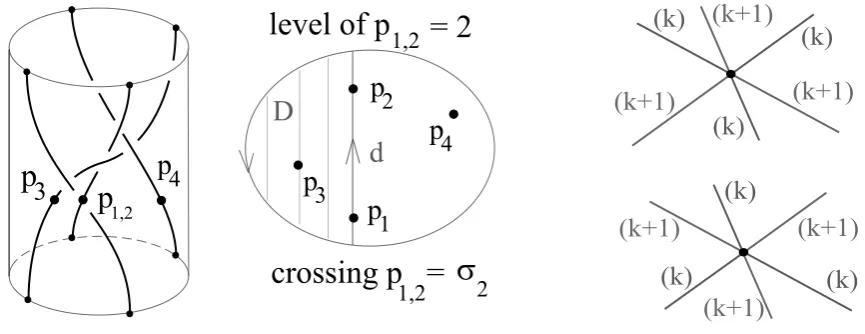
DEFINITION 3.5. Any point p TG( ) that is not a vertex corresponds to an

ordered pair (pi, pj) (Dx y z ). Let t be the time moment when pi, pj project

to the same point under pr_{x z} Ax z. Then rott( ) in a thin slice Dx y (z ,z )

looks like a braid generator k or k 1, all other strands do not cross each other, see

Fig. 12. The index k is called the level of the point p TG( ).

From another point of view we may compute the level of a crossing (pi,pj) as

fol-lows. Take the oriented straight segment d having endpoints on Dx y z and passing

Fig. 12. Levels in trace graphs of closed braids.

circuit bounding a disk D, see Fig. 12. The number of intersections IntD plus 1 is called the level (k) of the point p. We chose the name level since any crossing of prx z( ) is located at its horizontal level with respect to X.

Lemma 3.6. Going along a trace circle of a trace graph, the level of a point p may change only at a triple vertex as follows: k k 1, see Fig. 12.

Proof. The number of intersections of with the disk D from Definition 3.5 re-mains invariant until the segment d passes through other points of (Dx y z ) apart

from pi, pj defining p TG( ). While p passes through a triple vertex of TG( ),

the segment d intersects exactly one strand of , hence the number of points D changes by 1. This also follows from k k 1 k k 1 k k 1.

Orient the 2-dimensional torus ZT S1

z St1 in such a way that the first direction

is vertical along S1

z and the second one is horizontal opposite to St1.

DEFINITION 3.7. Let TG( ) be the trace graph of a closed braid , where

Bn. For each k 1, , n 1, denote by S(k) the k-th level subgraph consisting of

all edges having the level k. Orient each edge of TG( ) vertically along Sz1. A right

attractor is an oriented cycle RA(k) S(k) _{such that at each triple vertex, where two}

edges of S(k) _{go up, the cycle RA}(k) _{goes to the right. Denote by (q}(k)_,r(k)_{)the winding}

numbers of RA(k) in the vertical direction S1

z and reversed horizontal direction ( St1),

respectively. Let e(k) _S(k) _{ZT be the k-th level embedding induced by the torus}

pro-jection pr_zt S(k) _{TG( ) ZT S}1

z St1, see Lemma 3.8 (b) below.

Lemma 3.8. LetTG( ) be the trace graph of a closed braid ,where Bn.

(a) Any level subgraph S(k) _{has only trivalent vertices; at each vertex 1 edge goes}

down, 2 edges go up or vice versa with respect to the projection pr_z TG( ) S1

z.

(b) Any level subgraph S(k) _{projects 1-1 to its image under pr}

zt S(k) ZT.

(c) Subgraphs S(k) _{and S}(m) _{have common points under pr}

zt if and only if k m 1;

the adjacent subgraphs can meet only in triple vertices as in Fig. 12. (d) If k m 1 then the edges of S(k) _{cross over S}(m) _{under pr}

zt TG( ) ZT.

(e) Each level subgraph S(k) _{has at least one right attractor. Its vertical winding}

num-ber q(k) _{is positive. Any two right attractors in S}(k) _{have no common points.}

(f) Under the shift t t each level subgraph S(k) _{maps to the subgraph S}(n k)_.

Proof. (a) A triple vertex TG( ) corresponds to a triple intersection (qr s) of strands from , see Fig. 10. Let k be the level of the crossing p formed by the distant strands of q and s right below (qr s). By Lemma 3.4 (a) the crossing p is associated to a point below in the middle trace circle passing through . Right above p the crossings formed by the strands (qr) and (r s) have the same level k. The 3 other types of crossings have the same level k 1 or k 1, see Fig. 12.

(b) If the trace graph TG( ) has a crossing under the projection przt TG( )

ZT then the points forming the crossing have the same z-coordinate and different x-coordinates. Hence they correspond to 2 crossings of some diagram pr_{x z}(rott( )).

Definition 3.5 implies that the levels of these crossings differ at least by 2. The items (c) and (d) follow directly from the above arguments, see Fig. 13. (e) Starting with any vertex in S(k) and going always to the right in finitely many steps we will get a closed cycle oriented vertically, ie q(k) 0. If two right attractors in S(k) _{have a common vertex then they go along the same path and coincide.}

(f) Let a point p S(k) _{correspond to a pair (p}

i, pj) in a meridional disk

Dx y z V. The level k is equal to 1 plus the number of intersections IntD ,

see Fig. 12. Under t t , the pair (pi, pj) converts to (pj, pi), the disk D goes

to the complementary disk D Dx y z D. Then the level of (pj, pi) is 1 plus

the number of intersections IntD , i.e. 1 (n 2 (k 1)) n k.

4. Combinatorial encoding trace graphs up to isotopy

4.1. Reconstructing a closed braid from its trace graph. The moves on trace graphs are in Fig. 5 and Fig. 6. The trace graph of a closed braid in general position has the combinatorial features summarized below.

DEFINITION 4.1. An embedded finite graph G is a generic trace graph if

• under t t the graph G maps to its image under the symmetry in S1

z;

• _{G splits into trace circles monotonic with respect to prz G Sz}1_{, they should}

intersect in triple vertices of G and verify Lemmas 3.1, 3.4;

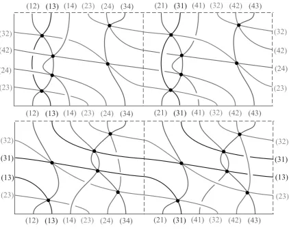
Fig. 13. Splittings of TG( 2 ₃2 2) and TG( 2 ₁2 2) into level

sub-graphs.

A smooth family of trace graphs Gs , s [0, 1], is called an equivalence if

• _{for all but finitely many moments s [0, 1], the trace graphs Gs are generic;} • at each critical moment, Gs changes by a trihedral or tetrahedral move.

An isotopy of trace graphs is an equivalence through generic trace graphs only.

Now we reconstruct a closed braid from its generic trace graph with markings.

Lemma 4.2. For a braid Bn, the closure V can be reconstructed up to

isotopy in the solid torus from its generic trace graph G with markings.

Proof. Consider a vertical section Pt G (Ax z t ) not containing vertices of

G. Then Pt is a finite set of points with markings (i j)[k], where k 1, , gcd(ni,nj) ,

see Lemma 3.1 (a). The points of Pt will play the role of crossings of a diagram of .

The labelled set Pt defines the Gauss diagram GDt as follows. Take mi 1Si1, split

each oriented circle S1

orientation. Mark several points in the q-th arc of S1

i in a 1-1 correspondence and the

same order with the points of Pt projected under prz Pt Sz1 and having labels (i j)[k]

or (ji)[k] for k 1, , gcd(ni,nj).

So each point of Pt gives 2 marked points in mi 1 Si1 labelled with (i j)[k] and

(ji)[k]. Connect them by a chord and get the Gauss diagram GDt. The zero Gauss

diagram GD0 is realizable by the given diagram of the closed braid . The Gauss

diagram GDt gives rise to a diagram of a closed braid isotopic to since the

trans-formation from GD0 to GDt is clearly realizable by an isotopy of closed braids.

Using Lemma 4.2, we state Theorem 1.4 in a slightly different form.

Proposition 4.3. Closed braids 0 and 1 are isotopic in the solid torus V if and

only if TG( 0) and TG( 1) are equivalent in the sense of Definition 4.1.

4.2. Trace codes of trace graphs. Any curve in ZT Sz1 St1 has a homology

class (u, ), where u is the winding number in the vertical direction S_z1, is the wind-ing number in the direction opposite to S1

t. Take a generic trace graph G from

Defin-ition 4.1.

DEFINITION 4.4. A cycle in a level subgraph S(k) G is calledtrivial if it bounds

a disc under the embeddinge(k) _S(k) _{ZT. Any trivial cycle has an orientation induced}

by the oriented torus ZT. Any non-trivial cycle can be oriented in such a way that its vertical (possibly, horizontal too) winding number is non-negative.

A level subgraph is said to bedegenerate, if all its non-trivial cycles have homology classes that are multiples of each other in H1(ZT) . Let a level subgraph S(k)

be non-degenerate. Denote by (q(k)_,r(k)_{) the homology class of a right attractor. Among}

all non-trivial cycles in S(k) _{choose maximal cycles with homology classes (u, ) such}

that the value M u q(k) r(k) is non-zero and maximal.

Recall that q(k) _{0 by Lemma 3.8 (e). If r}(k) _{0, then set M . The}

non-degenerate graph S(k) should contain non-trivial cycles with M 0. If there are maximal cycles with different homology classes, then take one with maximal vertical number u. Now the maximal homology class (u(k)_, (k)_{) of S(k) is well-defined.}

By Lemma 3.1 trace circles in a trace graph are distinguished by their markings. Any right attractor can be oriented in such a way that its vertical winding number is positive. So right attractors are encoded by cyclic words of vertices.

DEFINITION 4.5. Choose a base point in each trace circle of a generic trace graph

G. Enumerate all vertices of a trace circle T(ab)[i] G by (ab)[i]1, (ab)[i]2, . A triple

vertex G can be encoded by an ordered triplet (ab)[i](xk), (ac)[j](yk 1), (bc)[m](zk) .

The trace code TC contains the following 3 pieces of data.

• The second piece contains the homology classes (q(k)_,r(k)_{) of right attractors for}

each level subgraph S(k)_{, k 1, , n 1.}

• _{The third piece is the set of maximal homology classes (u}(k)_, (k)_{) introduced for}

each level subgraph S(k) in Definition 4.4, k 1, , n 1.

Two trace codes are called identical: TC1 TC2 if theirs three pieces coincide.

Our aim is to reconstruct the embedding of a generic closed trace graph G into the thickened torus from its trace code TC(G), see Lemma 5.1. Lemma 4.6 proves this for a level subgraph S(k) _{G. Recall that an isotopy in the torus ZT is a smooth}

family of diffeomorphisms Fs ZT ZT, where s [0, 1], F0 idZT.

Lemma 4.6. Let G be the trace graph of a closed braid , where Bn.

(a) The embedding e(k) S(k) ZT of a degenerate level subgraph S(k) G can be reconstructed by its ordered triplets and the homology class (q(k),r(k)) of its right at-tractor up to Dehn twists around a right atat-tractor and isotopy in ZT.

(b) The embedding e(k) _S(k) _{ZT of a non-degenerate level subgraph can be}

recon-structed up to isotopy in ZT by its ordered triplets, the homology class (q(k)_{, r}(k)_{) of}

its right attractor and the maximal homology class (u(k)_, (k)_{) of S}(k)_.

Proof. (a) A right attractor RA(k) S(k) _{can be recognized using the set of ordered}

triplets of vertices. Embed RA(k) into ZT according to its winding numbers (q(k)_{, r}(k)_).

Add other vertices and edges of S(k) _{to get an embedding of the connected component of}

S(k)_{containing the chosen attractor. If S}(k)_{is non-connected, there is another right attractor}

with the same homology class (q(k),r(k)).

We repeat the above steps for all connected components of S(k). The image of the resulting embedding is contained in one or several annuli with the prescribed homology class (q(k)_,r(k)_{). The whole embedding S}(k) _{ZT is well-defined up to Dehn twists}

around a right attractor and isotopy in ZT.

(b) For a non-degenerate subgraph S(k)_{, we construct an embedding S}(k) _{ZT as}

in (a). We have to improve this embedding by a suitable Dehn twist around a right attractor in such a way that the maximal homology class is (u(k), (k)).

The number of different homology classes is linear with respect to the number of vertices in S(k)_{. We look at non-trivial cycles in the constructed embedding. Let J}

be the algebraic intersection number of a right attractor RA(k) S(k) and a non-trivial cycle with a homology class (u, ).

The Dehn twist around RA(k) acts on the homology: (u, ) (u J q(k), Jr(k)). Then M u q(k) r(k) is invariant under all Dehn twists around RA(k). In the already embedded graph S(k) ZT we may recognize all non-trivial maximal cycles with the maximal value M computed using (u(k), (k)).

If there are two maximal cycles with different classes (u, ) and (u, ), then (u u) q(k) _{( ) r}(k) _{i, hence (u, ) (u, ) i(q}(k)_,r(k)_{) for some i. Since}

number J with the right attractor RA(k). So a Dehn twist around RA(k) acts on the set of the homology classes of all maximal cycles as a shift by J(q(k)_,r(k)_).

We know that among maximal cycles we can find one with the homology class (u(k)_, (k)_{), the vertical number u}(k) _{is maximal possible. Let (u, ) be the homology}

class of a maximal cycle C with the maximal vertical number u in the embedding S(k) ZT. There is an integer i such that (u(k), (k)) (u, ) i J(q(k), r(k)).

Thei Dehn twists around the right attractor RA(k) convert the cycleC into a required cycle C with the maximal class (u(k)_, (k)_{). The final embedding S}(k) _{ZT contains a}

basis consisting of C and RA(k) with the prescribed homology classes. Therefore the embedding is well-defined up to isotopy in ZT.

If all level subgraphs of G are non-degenerate, we may forget about levels in the trace code TC(G). The subgraphs S(k) _{G should be connected and two adjacent}

sub-graphs meet at each triple vertex, see Lemma 3.8 (c). Hence the levels of subsub-graphs can be reconstructed up to the inversion (1, 2, ,n 1) (n 1, , 2, 1), which cor-responds to the time shift t t . In the second and third pieces of TC(G) we may leave only the homology class of a right attractor RA(1) and the maximal homology class (u(1), (1)) of the first level subgraph S(1).

5. Recognizing trace graphs in polynomial time

5.1. Recognizing trace graphs up to isotopy.

Lemma 5.1. Two generic trace graphs G0 and G1 are isotopic in the thickened

torus if and only if their trace codes TC(G0) and TC(G1) become identical after

suitable cyclic permutations of vertices in trace circles.

Proof. The part only if follows from the fact that the trace code is invariant under isotopy in . The part if says that the embedding of a trace graph G into the thickened torus Ax z St1 can be reconstructed from its trace code.

By Lemma 4.6 we may reconstruct embeddings of level subgraphs S(k) _{G into}

the torus ZT. Two embeddings of S(1) _{and S}(2) _{can be joint together since the union}

S(1) S(2) should be embedded into ZT by Lemma 3.8 (c). The resulting embedding is well-defined up to isotopy in ZT provided that either one of the subgraphs S(1) and S(2) _{is non-degenerate or their right attractors have distinct homology classes.}

We embed the third subgraph S(3) _{into ZT to get a joint embedding S}(2) _S(3) _ZT

as above. The union S(1) _S(2) _S(3) _{can be already considered as an embedding into}

the thickened torus since the edges of S(3) should cross over S(1) in ZT.

The final embedding G is well-defined up to isotopy if either one of the sub-graphs S(k) _{is non-degenerate or there are two right attractors with different homology}

classes. Otherwise all S(k) _{are degenerate and the embedding G is invariant under}

Proposition 5.2 gives a (surprisingly) polynomial algorithm recognizing complicated topological objects: trace graphs up to isotopy in a thickened torus.

Proposition 5.2. Let , Bn be braids of length l. There is an algorithm

of complexity C(n 2)n2 ₈

(6l)n2 _{n 1}

to decide whether TG( ) and TG( ) are isotopic in the thickened torus , where the constant C does not depend on l and n. In the case of pure braids, the power n2 _{8 can be replaced by 1. If the closure of a braid is}

a knot, a single circle in the solid torus, then the complexity reduces to Cn(6l)n 1_.

Proof. By Lemma 2.1 we may assume that the trace graphs TG( ), TG( ) have Q 2l(n 2) triple vertices. If we fix numbers k in markings (i j)[k] with i j and a base point in each trace circle then we can construct trace codes TC( ), TC( ) of TG( ), TG( ), see Definition 4.5. The trace codes TC( ), TC( ) can be compared in linear time with respect to the number Q of triple vertices.

By Lemma 3.1 (a) the graph TG( ) splits into N( ) trace circles. Denote by k1, ,kN( ) the number of triple vertices in the trace circles of TG( ). Then there are

exactly k1k2 kN( ) choices of base points in the trace cirles. Since k1 kN( )

3Q 6l(n 2), we have

k1k2 kN( )

k1 kN( )

N( )

N( )

6l(n 2) N( )

N( )

(6l)n2 n

due to the estimates n 1 N( ) n(n 1) from Lemma 3.1 (b).

Let (n1, ,nm) be the lengths of cycles of the induced permutation Sn. There

are n 2 non-trivial cycles with lengths ni 1. For each pair of non-trivial cycles

with lengths (ni, nj), there are gcd(ni,nj) choices of numbers k in markings (i j)[k],

i.e. totally i jgcd(ni,nj). Since the number of pairs is n₂2 and gcd(ni,nj) n 2,

the number of choices (n 2)(n22) (n 2)n2 8 1 for n 4.

With a fixed choice of markings and base points, we check whether TC( ) TC( ) with complexity Cl(n 2). So, the final complexity of the algorithm is C(n 2)n2 8(6l)n2 n 1. For pure braids, markings (i j) without [k] are well-defined and we may replace n2 _{8 by 1. If is a knot, then N( ) n 1, markings [k] 1, ,}

n 1 are well-defined and the complexity reduces to Cn(6l)n 1_.

5.2. Recognizing trace graphs up to trihedral moves. Now we extend Prop-osition 5.2 to recognize trace graphs up to trihedral moves.

DEFINITION 5.3. Let G be a generic trace graph from Definition 4.1. A

Fig. 14. Simulation of the appearance of a trihedron.

Lemma 5.4. Let TG( ), TG( ) be reduced trace graphs of closed braids , , respectively. The original trace graphs TG( ), TG( ) are equivalent through trihedral moves if and only if the reduced graphs TG( ), TG( ) are isotopic in .

Proof. The part if is trivial since reduced graphs are obtained by trihedral moves. The part only if. The given equivalence between the original graphs provides an equivalence Gs through trihedral moves only, where s [0, 1], G0 TG( ) and G1

TG( ). The trihedral moves in Gs can create or delete only embedded trihedra. We

simulate the creation of each trihedron T as shown in Fig. 14.

Either T will disappear completely by a further trihedral move in Gs or an

ad-jacent trihedron will be deleted and will destroy T. In both cases we miss the deleting move in the simulation. After simulating all trihedral moves the equivalence Gs

be-comes a required isotopy between reduced graphs.

Proof of Theorem 1.5. Embedded trihedra in a trace graph can be recognized in quadratic time with respect to the number of vertices. For each pair of vertices, we check if they are connected by three edges not containing other vertices. After that the algorithm of Proposition 5.2 can be applied to the reduced trace graphs TG( ), TG( ) and gives the required polynomial complexity in the braid length.

A meridional quadrisecant of a closed braid in the solid torus V is a straight line in a meridional disk Dx y z meeting in 4 points. For an equivalence s

without meridional quadrisecants, the canonical loops of rotated braids rott( s) can pass

only through ✟☎ ✆ ✞

✝, ✆✞and can touch !❅, see Subsection 2.1. Passing through ✦❛☞☞▲▲

creates a a meridional quadrisecant in a closed braid. Passing through a tangency with

!

❅ corresponds to a trihedral move in Fig. 5.

Corollary 5.5. Let , Bn be braids of length l. There is an algorithm

of complexity C(n 2)n2 8(6l)n2 n 1 to decide whether there is an equivalence s such

that CL( s) can pass only through ✟☎

✆ ✞

Proof. The closed braids , are equivalent in the above sense if and only if their trace graphs TG( ), TG( ) are equivalent through trihedral moves only. So the algorithm of Theorem 1.5 can be applied to TG( ), TG( ).

The following conjecture implies that, for closed braids having trace graphs with-out trihedra, the conjugacy problem can be solved in a polynomial time similarly to Theorem 1.5 since tetrahedral moves do not change the number of triple vertices.

Conjecture 5.6. If trace graphs of isotopic closed braids have no trihedra then they are related by tetrahedral moves only.

The idea is to simplify an equivalence of trace graphs cancelling moves that create and remove trihedra. The ultimate aim is to extend Conjecture 5.6 to all closed braids making an equivalence of trace graphs monotone with respect to the number of triple vertices, which would give a polynomial algorithm for all braids.

6. A geometric recognizing 3-braids up to conjugacy

According to González-Meneses [11], if two braids and satisfy k k in Bn

for some k 0, then and are conjugate. It follows that braids and are con-jugate if and only if k and k are conjugate for some k 0, see González-Meneses [11, Corollary 1.2]. For any braid Bn, there is a power k such that the permutation

k _S

n induced by k is trivial, hence k is pure. So the conjugacy problem for the

braid group Bn reduces to the case of pure braids.

6.1. Cyclic invariants based on 3-subbraids. In this subsection we recognize closed pure 3-braids up to isotopy in the solid torus by using invariants of their trace graphs calculable in a linear time with respect to the braid length. Then trace circles in the trace graph TG( ) can be denoted simply by T(i j), where i, j 1, ,n . We

shall define cyclic invariants depending on 3-subbraids of and distinguishing all pure 3-braids up to conjugacy.

Take a pure braid Bn and enumerate the components of by 1, ,n. Fix

three pairwise disjoint indices i, j,k 1, ,n . We shall define the cyclic invariants C(i j) depending on the 3-subbraid i jk based on the strands i, j,k.

DEFINITION 6.1. Take the reduced trace graph TG( i jk) well-defined up to

iso-topy of i jk by Lemma 5.4 since tetrahedral moves are not applicable for 3-braids. For

each triple vertex T(i j), we write the ordered triplet of the markings of trace circles

passing through in the order from left to right below , see Fig. 16. The vertices and their triplets are ordered vertically in the direction S1z. Then C(i j)( ) is a vertical

Fig. 15. Trace graphs of the Borromean links: ( 1 21)3 and 2

Due to the symmetry of TG( ) under the shift t t , the other invariants C(ji), C(ki),C(k j) can be reconstructed from the already defined ones.

EXAMPLE 6.2. Fig. 15 contains the trace graphs of the closures of the 3-braids

( 1 ₂1)3 and ₁2 ₂2 ₁2 ₂ 2. Both closures are Borromean links, i.e. the braids are

con-jugate. In fact the second graph is isotopic to the first one by eliminating the couple of embedded trihedra. The cyclic invariants C(12),C(13),C(23) are shown below the

pic-tures. The vertices of the embedded trihedra in the second trace graph are encoded by (12)(13)(23) and (23)(13)(12), i.e. the extreme markings swap their positions. More-over, the cyclic invariants show that the braids are not trivial.

6.2. Recognizing 3-braids up to conjugacy in a linear time.

Lemma 6.3. Number components of two closed pure 3-braids , by 1, 2, 3. Suppose that the ordered links , are isotopic in the solid torus V . Then the cyclic invariants C(i j)( ) and C(i j)( ) coincide for all disjoint i, j 1, 2, 3 . The invariant

C(i j)( ) is calculable in linear time with respect to the length of .

Proof. By Proposition 4.3 the trace graphs of isotopic closed braids are connected by an isotopy in the thickened torus , trihedral moves and tetrahedral moves. The cyclic invariants are not changed under isotopy of trace graphs. Tetrahedral moves are not applicable for 3-braids. Trihedral moves create trihedra that are recognizable by cyclic invariants and deleted in the construction of Definition 6.1. To compute C(i j)( )

we need to look at all triple vertices of the trace circle T(i j). The total number of

ver-tices is not more than 2l by Lemma 2.1.

Recall that closed pure 2-braids are classified up to conjugacy by the linking num-ber lk12 of closed strands 1 and 2. Proposition 6.4 implies that 3-braids can be

recog-nized up to conjugacy in linear time with respect to their length.

Proposition 6.4. Fix closed pure 3-braids , with ordered components. The braids , are conjugate if and only if the linking numbers lk12( ) lk12( ) and

the cyclic invariants C(12)( ), C(12)( ) coincide up to cyclic permutation.

Proof. The part only if is Lemma 6.3. The part if says the original 3-braid can be reconstructed from its invariants lk12 and C(12). Simply assume that lk12 0, e.g. strands

1, 2 are straight, i.e. multiply both braids by 2 lk12_{, where (}

1 2)3.

Consider a meridional disk Dz Dx y z in the solid torus V, where the closed

braid lives. Mark the intersection points Dz by 1, 2, 3 according to the

compo-nents of . Since points 1, 2 do not move in Dz while z varies, we need to know only

Fig. 16. Dynamic interpretation of triple vertices.

In Fig. 16 the arrow at point 3 shows its meridional velocity while z increases. In the left hand side picture, the line connecting points 1, 3 is going to have a positive slope in Dz, hence the trace circle T(31) is increasing as a function z(t). So triplets

describe neighbourhoods of associated triple vertices, which can be joined together to get a complete trace graph leading to a braid by Lemma 4.2.

ACKNOWLEDGEMENTS. The second author is especially grateful to Hugh Morton

for fruitful suggestions. He also thanks M. Kazaryan, V. Vassiliev for useful discussions. We thank the anonymous referee for critical comments and valuable improvements.

References

[1] J.S. Birman: Braids, Links, and Mapping Class Groups, Ann. of Math. Studies 82, Princeton Univ. Press, Princeton, N.J., 1974.

[2] J.S. Birman, V. Gebhardt and J. González-Meneses: Conjugacy in Garside groupsI, cyclings, powers and rigidity, Groups Geom. Dyn.1(2007), 221–279.

[3] J.S. Birman, V. Gebhardt and J. González-Meneses: Conjugacy in Garside groups II,structure of the ultra summit set, Groups Geom. Dyn. 2(2008), 13–61.

[4] J.S. Birman, V. Gebhardt and J. González-Meneses: Conjugacy in Garside groupsIII,periodic braids, J. Algebra316(2007), 746–776.

[5] J.S. Carter and M. Saito: Knotted Surfaces and Their Diagrams, Mathematical Surveys and Monographs55, Amer. Math. Soc., Providence, RI, 1998.

[6] T. Fiedler: Gauss Diagram Invariants for Knots and Links, Mathematics and its Applications 532, Kluwer Acad. Publ., Dordrecht, 2001.

[7] T. Fiedler: One-parameter knot theory, preprint, University of Toulouse III (March 2003). [8] T. Fiedler and V. Kurlin: Fiber quadrisecants in knot isotopies, J. Knot Theory Ramifications

17 (2008), 1415–1428.

[9] T. Fiedler and V. Kurlin: A one-parameter approach to links in a solid torus, J. Math. Soc. Japan 62 (2010), 167–211.

[11] J. González-Meneses: The nth root of a braid is unique up to conjugacy, Algebr. Geom. Topol. 3(2003), 1103–1118.

[12] A. Hatcher: Topological moduli spaces of knots, arXiv:math.GT/9909095.

[13] K.H. Ko and J.W. Lee: A fast algorithm to the conjugacy problem on generic braids; Chapter 16 in Proceedings of the International Workshop on Knot Theory for Scientific Objects (March 2006), OCAMI Studies1.

[14] K. Murasugi: On Closed 3-Braids, Memoirs of the American Mathmatical Society151, Amer. Math. Soc., Providence, RI, 1974.

Thomas Fiedler

Laboratoire Emile Picard Université Paul Sabatier

118 route Narbonne, 31062 Toulouse France

e-mail: [email protected] Vitaliy Kurlin

Department of Mathematical Sciences Durham University

Durham DH1 3LE United Kingdom