Mutant knots with symmetry

Mutant knots with symmetry

Department of Mathematical Sciences, University of Liverpool, Peach Street, Liverpool L69 7ZL, UK.

Abstract

Mutant knots, in the sense of Conway, are known to share the same Homfly polynomial. Their 2-string satellites also share the same Homfly polynomial, but in general theirm -string satellites can have different Homfly polynomials for m >2. We show that, under conditions of extra symmetry on the constituent 2-tangles, the directedm-string satellites of mutants share the same Homfly polynomial for m <6 in general, and for all choices ofmwhen the satellite is based on a cable knot pattern.

We give examples of mutants with extra symmetry whose Homfly polynomials of some 6-string satellites are different, by comparing their quantum sl(3) invariants.

1. Introduction

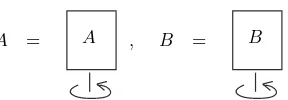
This paper has been inspired by recent observations of Ochiai and Jun Murakami about the Homfly skein theory of m-parallels of certain symmetrical 2-tangles. In [8] Ochiai remarks that the 3-parallels of the tangle AB in figure 1 and its mirror image

AB=BAare equal in the Homfly skein of 6-tangles, in other words, in the Hecke algebra

H6, [1].

A

B

=

Fig. 1. The 2-tangleABused by Ochiai

As a consequence, the 3-parallels of any mutant pair of knots given by composing the 2-tanglesABandBAwith any other 2-tangleCand then closing, as in figure 3 will share the same Homfly polynomial. This is in contrast with the known fact that 3-parallels of mutant knots in general can have different Homfly polynomials, [7, 4].

There is interest in the extent to which the Homfly polynomial ofm-parallels or other

m-string satellites can distinguish mutants which are closures ofABC andBACwithA

andB as above. Ochiai has found that the 4-parallels ofABandBAare different in the skeinH8.

The purpose of this paper is to show that ifA andB are any two oriented 2-tangles which have the symmetry shown in figure 2 then them-parallels, and indeed any directed

m-string satellite, of knots bABC and bBAC shown in figure 3 share the same Homfly polynomial provided thatm <6. In contrast there exist examples ofA, BandC where

A = A _, B = B

Fig. 2. The symmetry imposed on the tanglesAandB

K =

A

B

C K′ ₌

B

A

C

Fig. 3. Tangle interchange

A = , B = ,

for which the Homfly polynomials of the 6-fold parallel of K and K′ _{are different. The}

simplest such example, the pretzel knots shown in figure 8, uses Ochiai’s choice of sym-metric tangles AandB.

In an unexpected extension of the main result we show that the Homfly polynomial of a genuine connected cable, based on the (m, n) torus knot pattern, with m and n

coprime, will not distinguish mutants with symmetry above, forany number of strings,

m, although a more general connected satellite pattern can do so.

The examples which exhibit differences for the directly oriented 6-parallel can also be used to show that the 4-parallels with two pairs of reverse strands have distinct Homfly polynomials.

The proofs are based on the relation of the Homfly satellite invariants to quantumsl(N) invariants, and the techniques are an extension of work with Cromwell [4] and with H. Ryder [6]. The eventual calculations that exhibit the difference of invariants in the specific example depend on the 27 dimensional irreducible module over sl(3) corresponding to the partition 4,2, and some Maple calculations following similar lines to those in [6].

2. Shared invariants of mutants

The termmutant was coined by Conway, and refers to the following general construc-tion.

Suppose that a knotK can be decomposed into two oriented 2-tanglesF andG

A new knot K′ _{can be formed by replacing the tangleF with the tangleF}′ _=τ

i(F)

given by rotatingF throughπin one of three ways,

τ1(F) = F , τ2(F) = F , τ3(F) = F ,

reversing its string orientations if necessary. Any of the three knots

K′ _{= τ}

i(F) G

is called amutant ofK.

The two 11-crossing knots,C andKT, found by Conway and Kinoshita-Teresaka are the best-known example of mutant knots. These two knots are shown in figure 4.

C = KT =

Fig. 4. The Conway and Kinoshita-Teresaka mutant pair

2·1. Satellites

A satellite ofK is determined by choosing a diagramQin the standard annulus, and then drawingQon the annular neighbourhood ofKdetermined by the framing, to give the satellite knotK∗Q. We refer to this construction asdecorating K with the pattern

Q, as shown in figure 5.

Q= K= K∗Q=

Fig. 5. Satellite construction

For fixed Q the Homfly polynomial P(K∗Q) of the satellite is an invariant of the framed knot K. The invariants P(K ∗Q) as Q varies make up the Homfly satellite invariants of K. We use the alternate notationP(K;Q) in place ofP(K∗Q) when we want to emphasise the dependence onK.

The general symmetry result compares the invariants of two knotsKandK′_{made up}

Theorem 1. Suppose that A and B are both symmetric under the half-twist τ3, so

that

A = A , B = B

Let K and K′ _{be knots which are the closure of ABC and BAC respectively for any}

tangle C, as in figure 3. Then P(K∗Q) =P(K′_{∗Q)for every closed braid pattern Q}

on m <6 strings.

Remark 1. _{The proof applies equally to the case whereQis the closure of any directly}

oriented m-tangle with m <6.

In order to prove the theorem we must rewrite the Homfly satellite invariants in terms of quantum sl(N) invariants, so we now give a brief summary of the relations between these invariants, originally established by Wenzl. Further details can be found in [1] and the thesis of Lukac, [3], including details of variant Homfly skeins with a framing correction factor, x. These are isomorphic to the skeins used here but the parameter allows a careful adjustment of the quadratic skein relation to agree directly with the natural relation arising from use of the quantum groupssl(N).

2·2. Homfly skeins

For a surface F with some designated input and output boundary points the (linear) Homfly skein of F is defined as linear combinations of oriented diagrams in F, up to Reidemeister moves II and III, modulo the skein relations

(i) − = (s−s−1_{) ,}

(ii) = v−1 _{, = v .}

It is an immediate consequence that

= δ ,

whereδ=v

−1_−v

s−s−1 ∈Λ. The coefficient ring Λ is taken asZ[v

±1_{, s}±1_{], with denominators}

sr_−s−r_{, r≥1.}

The skein of the annulus is denoted by C. It becomes a commutative algebra with a product induced by placing one annulus outside another.

The skein of the rectangle with minputs at the top andm outputs at the bottom is denoted byHm. We define a product inHm by stacking one rectangle above the other,

obtaining the Hecke algebraHm(z), whenz=s−s−1 and the coefficients are extended

to Λ. The Hecke algebraHm can also be regarded as the group algebra of Artin’s braid

groupBm generated by the elementary braidsσi,i= 1, . . . , m−1, modulo the further

quadratic relationσ2

i =zσi+ 1.

The closure map from Hm to C is the Λ-linear map induced by mapping a tangleT

to its closure Tb in the annulus (see figure 6). We refer to a diagramQ=Tbas adirectly oriented pattern.

The image of this map is denoted by Cm, which has a useful interpretation as the

b

T = _T

Fig. 6. The closure map

Moreover, the submodule C+ ⊂ C spanned by the union∪m≥0Cm is a subalgebra ofC

isomorphic to the algebra of the symmetric functions.

2·3. Quantum invariants

A quantum groupG is an algebra over a formal power series ring Q[[h]], typically a deformed version of a classical Lie algebra. We write q=eh_{, s=e}h/2 _{when working in} sl(N)q. A finite dimensional module overG is a linear space on whichGacts.

Crucially, G has a coproduct ∆ which ensures that the tensor productV ⊗W of two modules is also a module. It also has a universalR-matrix (in a completion ofG ⊗ G) which determines a well-behaved module isomorphism

RV W :V ⊗W →W⊗V.

This has a diagrammatic view indicating its use in converting coloured tangles to module homomorphisms.

W ⊗ V

V ⊗ W RV W

A braid β on m strings with permutation π ∈Sm and a colouring of the strings by

modulesV1, . . . , Vm leads to a module homomorphism

Jβ :V1⊗ · · · ⊗Vm→Vπ(1)⊗ · · · ⊗Vπ(m)

usingR±1Vi,Vj at each elementary braid crossing. The homomorphismJβ dependsonly on

the braid β itself, not its decomposition into crossings, by the Yang-Baxter relation for the universalR-matrix.

WhenVi=V for alliwe get a module homomorphismJβ :W →W, whereW =V⊗m.

Equally, a directedm-tangleT determines an endomorphismJT ofW =V⊗m. Now any

sl(N) module W decomposes as a direct sumL(Wµ⊗Vµ(N)), where Wµ is the linear

subspace consisting of thehighest weight vectorsof typeµassociated to the moduleVµ(N).

Highest weight subspaces of each type are preserved by module homomorphisms, and so

JT determines (and is determined by) the restrictionsJT(µ) :Wµ→Wµ for eachµ.

If a knotKis decorated by a patternQwhich is the closure of anm-tangleT then its quantum invariantJ(K∗Q;V) can be found from the endomorphismJT ofW =V⊗m

in terms of the quantum invariants ofK and the highest weight mapsJT(µ) :Wµ→Wµ

by the formula

J(K∗Q;V) =XcµJ(K;Vµ(N)) (2·1)

with cµ= trJT(µ). This formula follows from lemma II.4.4 in Turaev’s book [11]. Here

Proof of theorem 1 Take V = V(N) _{as the fundamental module of dimension N for} sl(N). Then the only highest weight typesµwhich occur in equation (2·1) are partitions ofm with at mostN rows. BecauseJ(K∗Q;V(N)_{) =P(K∗Q) whenv =s}−N _{we can}

show thatP(K∗Q) =P(K′_{∗Q) by showing thatJ(K∗Q;V}(N)_{) =J(K}′_∗Q;V(N)_{) for}

allN. By equation 2·1 it is then enough to show thatJ(K;Vµ(N)) =J(K′;Vµ(N)) for all

N and all partitionsµ⊢m.

Now each tangleAandBdetermines an endomorphismJA, JBofVµ⊗Vµ. IfJAandJB

commute thenJ(K;Vµ) =J(K′;Vµ). The endomorphismsJAandJB are determined by

their restrictionJA(ν), JB(ν) to the highest weight subspacesWν in the decomposition

Vµ⊗Vµ =PWν⊗Vν, so it is enough to show thatJA(ν) andJB(ν) commute whereVν

is a summand ofVµ⊗Vµ. This is certainly the case for allν whereWν is 1-dimensional,

which includes the case of single row or column partitionsµ, [4].

As a special case of the work of Rosso and Jones, [9,5], we know that the endomorphism ofVµ⊗Vµ for the full twist ∆2 on two strings operates as a scalaref(ν) on each highest

weight space Wν, while the half twist ∆, represented by the R-matrix RVµVµ, operates

onWν with two eigenvalues±e21f(ν).

The positive and negative eigenspaces correspond to the classical decomposition of the Schur function (sµ)2into symmetric and skew-symmetric parts, h2(sµ) ande2(sµ), and

the dimension of each eigenspace of Wν is the multiplicity of sν in h2(sµ) and e2(sµ)

respectively.

Now A=τ3(A), so that A∆ = ∆A. Hence the endomorphismJA, and similarlyJB,

preserves the positive and negative eigenspaces of each Wν. If these eigenspaces have

dimension 1 or 0 thenJAandJB will commute onWν.

The theorem is then established by checking that nosν occurs inh2(sµ) ore2(sµ) with

multiplicity>1 for anyµwith|µ| ≤5. The decomposition of all of these can be quickly confirmed using the Maple program SF of Stembridge [10].

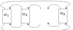
Corollary 2. Examples include thek-pretzel knotsK(a1, . . . , ak)with odd ai shown

in figure 7, where the numbers of half-twists ai can be permuted without changing the

Homfly polynomial of any satellite with≤5-strings.

a1 a2 ak

Fig. 7. The pretzel knotK(a1, . . . , ak)

3. Satellites with different Homfly polynomials

A further check with the program SF when |µ| = 6 shows that there are just three partitions,µ= 4,2, its conjugateµ = 2,2,1,1 and µ= 3,2,1 whose symmetric square

h2[sµ] contains summands with multiplicity > 1, as does the exterior squares of µ =

3,2,1. Explicitly h2[s4,2] = s8,4+s8,2,2+s7,4,1+s7,3,2+s7,3,1,1+s6,6+s6,5,1+

2s6,4,2+s6,3,2,1+s6,2,2,2+s5,5,1,1+s5,4,3+s5,4,2,1+s5,3,3,1+s4,4,4+s4,4,2,2. This

means that, althoughm-string satellites ofKandK′ _{must share the Homfly polynomial}

K = , K′ ₌

Fig. 8. The pretzel knotsK=K(1,3,3,−3,−3) andK′_{=K(1,3,−3,3,−3)}

Theorem 3. _{Let K and K}′ _{be the pretzel knots K = K(1,3,3,−3,−3) and K}′ ₌ K(1,3,−3,3,−3) shown in figure 8. The6-fold parallels K∗Q andK′_{∗Q, where Q is}

the closure of the identity braid on6 strings, have different Homfly polynomials.

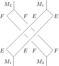
Proof. WriteK andK′ _{as the closure of the products ∆ABAB and ∆BAAB}

respec-tively, where

A = , B = ,

are the partially closed 3-braids shown, and ∆ is the positive half-twist. We show that

P(K∗Q) 6= P(K′ _{∗Q) when v = s}−3_{. These values are given by the sl(3) quantum}

invariantsJ(K∗Q;V(3)_{) andJ(K}′_∗Q;V(3)_{), whereV}(3)_{is the fundamental 3-dimensional}

module forsl(3). Since Qis the closure of the identity braid on 6 strings it induces the identity endomorphism on the module (V(3)₎⊗6_{. This module decomposes as}L_W

µ⊗Vµ(3)

where µruns through partitions of 6 with at most 3 rows. The trace of the identity on

Wµ is just dµ= dimWµ, giving

J(K∗Q;V(3)) =XdµJ(K;Vµ(3)).

The only partitionµin this range for which the exterior or symmetric square contains highest weight vectors of multiplicity >1 is the partition µ = 4,2, since the partition

µ = 2,2,1,1 has 4 rows and the repeated factors for µ = 3,2,1 occur for partitions with more than 3 rows. Now JA(µ)JB(µ) =JB(µ)JA(µ) for all otherµsinceA and B

are symmetric up to altering the framing on both strings, while maintaining the writhe. Then

P(K∗Q)−P(K′∗Q) =dµ(J(K;Vµ(3))−J(K

′

;Vµ(3)))

when v = s−3 _{and µ = 4,2. Since d}

µ 6= 0 it is enough to show that J(K;Vµ(3)) 6=

J(K′_;V(3)

µ ). The moduleVµ(3) has dimension 27.

We now work in the quantum group sl(3) and drop the superscript (3) from the irreducible modules.

Decompose the moduleVµ⊗VµasPWν⊗Vν and compare the endomorphisms given

by the tangles T=ABAB∆ andT′_=BAAB∆.

In this case just one of the invariant subspaces of highest weight vectors has dimension

>1. It can be shown that the corresponding 2×2 matricesAµandBµarising from the two

mirror-image tanglesAandBwith 3 crossings satisfy tr(AµBµAµBµ−AµAµBµBµ)6= 0,

which results in a difference in their sl(3) invariantsJ(K;Vλ).

3·1. Use of the quantum groupsl(3)q

The calculation of the 2×2 matricesAν andBν giving the effect of the two tangles

on the highest weight vectors where there is a 2-dimensional highest weight subspace of the symmetric part of the module depends on finding the explicit action of the quantum group on the 27-dimensional module Vµ(3) with µ = 4,2 and its tensor square, as well

as the homomorphism representing its R-matrix. I used the linear algebra packages in Maple to handle the matrix working and subsequent polynomial factorisation, following fairly closely the techniques developed with H. Ryder in the paper [6].

In the interests of reproducibility I give an account of the methods used, and some of the checks applied during the calculations, to test against known properties.

We start from a presentation of the quantum group sl(3)q as an algebra with six

generators,X± 1 , X

±

2, H1, H2, and a description of the comultiplication and antipode.

Let M be any finite-dimensional left module over sl(3)q. The action of any one of

these six generators Y will determine a linear endomorphism YM of M. We build up

explicit matrices for these endomorphisms on a selection of low-dimensional modules, using the comultiplication to deal with the tensor product of two known modules, and the antipode to construct the action on the linear dual of a known module. We must eventually determine the matricesYM for our moduleM =V , and find the 729×729

R-matrix,RMM which represents the endomorphism ofM⊗M needed for crossings.

We follow Kassel in the basic description of the quantum group from using generators

H1 and H2 for the Cartan sub-algebra, but with generatorsXi± in place of Xi andYi.

We use the notation Ki = exp (hHi/4), and set a= exp (h/4), s= exp (h/2) =a2 and

q= exp (h) =s2_{, unlike Kassel. The generators satisfy the commutation relations}

[Hi, Hj] = 0, [Hi, Xj±] =±aijXj±, [X

+

i , X

−

i ] = (K

2

i −Ki−2)/(s−s

−1_),

where (aij) =

2 −1

−1 2

is the Cartan matrix forSU(3) (and also the Serre relations

of degree 3 betweenX1± andX ± 2).

Comultiplication is given by

∆(Hi) =Hi⊗I+I⊗Hi,

(so ∆(Ki) =Ki⊗Ki,)

∆(Xi±) =X

±

i ⊗Ki+Ki−1⊗X

±

i ,

and the antipodeS byS(Xi±) =−s±1X

±

i ,S(Hi) =−Hi,S(Ki) =Ki−1.

The fundamental 3-dimensional module, which we denote byE, has a basis in which the quantum group generators are represented by the matrices YE as listed here.

X₁+=





0 1 0

0 0 0

0 0 0



, X₂+=





0 0 0

0 0 1

0 0 0





X1−= 



0 0 0

1 0 0

0 0 0



, X2−= 



0 0 0

0 0 0

0 1 0





H1= 



1 0 0

0 −1 0

0 0 0



, =





0 0 0

0 1 0

0 0 −1



For calculations we keep track of the elements Ki rather thanHi, represented by

K1= 



a 0 0 0 a−1 ₀

0 0 1



, K2= 



1 0 0

0 a 0

0 0 a−1 



for the module E.

We can then write down the elementsYEE for the actions of the generatorsY on the

moduleE⊗E, from the comultiplication formulae. TheR-matrixREE can be given, up

to a scalar, by the prescription

REE(ei⊗ej) =ej⊗ei, ifi > j,

=s ei⊗ei, ifi=j,

=ej⊗ei+ (s−s−1)ei⊗ej, ifi < j,

for basis elements{ei} ofE.

The linear dualM∗ _{of a moduleM becomes a module when the action of a generator} Y on f ∈ M∗ _{is defined by < Y}

M∗f, v >=< f, S(YM)v >, for v ∈ M. For the dual

moduleF =E∗ _{we then have matrices for Y}

F, relative to the dual basis, as follows.

X1+= 



0 0 0

−s 0 0

0 0 0



, X2+= 



0 0 0

0 0 0

0 −s 0





X1−= 



0 −s−1 ₀

0 0 0

0 0 0



, X2−= 



0 0 0

0 0 −s−1

0 0 0





K1= 



a−1 _{0 0}

0 a 0

0 0 1



, K2= 



1 0 0

0 a−1 ₀

0 0 a



.

The most reliable way to work out theR-matricesREF, RF E and RF F is to combine

REE with module homomorphisms cupEF, cupF E, capEF and capF E between the

mod-ulesE⊗F,F⊗Eand the trivial 1-dimensional module,I, on whichXi±acts as zero and

Ki as the identity. The matrices are determined up to a scalar by such considerations; a

choice for one dictates the rest.

Once these matrices have been found they can be combined with the matrix R−1_EE

to construct the R-matricesREF, RF E, RF F, using the diagram shown in figure 9, for

example, to determineREF as

REF = (1F⊗1E⊗capEF)◦(1F⊗R−1_EE⊗1F)◦(cupF E⊗1E⊗1F).

E F

E F

E F

E F

F E E F

F E

F E

=

Fig. 9. Construction of theR-matrixREF

submodule ofV ⊗V , while the two 6-dimensional modulesV andV are themselves submodules ofE⊗Eand F⊗F respectively.

We know, by the Pieri formula, that there is a direct sum decomposition ofV ⊗V

as M ⊕N, where M =V and N is the sum of the 8-dimensional module V and the 1-dimensional trivial module.

We first identify the module V as a submodule of E⊗E, knowing that E⊗E is isomorphic to V ⊗F. The full twist element on the two strings both coloured byE

is represented by R2

EE which acts onE⊗E as a scalar on each of the two irreducible

submodulesV andF.

Use Maple to find bases for the two eigenspaces of R2

EE. Then we can identify V

with the 6-dimensional one, and writeP and Qfor the 9×6 and 9×3 matrices whose columns are these bases. The partitioned matrix (P|Q) is invertible, and its inverse, found

by Maple, can be written as

R S

, whereRis a 6×9 matrix withRP =I6andRQ= 0.

RegardP= injM1EE as the matrix representing the inclusion of the moduleV into E⊗E. Then R = projEEM1 is the matrix, in the same basis, of the projection from E⊗E to V . ForM1=V the module generatorsYM₁ are given byYM₁ =R YEEP,

giving the explicit action of the quantum group onV .

We perform a similar calculation onF⊗F to identify the moduleM2=V and the

matrices injM2F F and projF F M2, giving the action of the quantum group onM2=V

in a similar way.

We use inclusion and projection further to find the four 62_×62 _{R-matrices R}

MiMj.

For example, to construct RM1M2 : M1⊗M2 → M2⊗M1, first map M1 ⊗M2 to

E ⊗E ⊗F ⊗F by injM1EE⊗injM2F F. Then construct the R-matrix crossing two

strings with E⊗E and two withF⊗F as the composite of 1⊗REF⊗1 ,REF ⊗RF E

and 1⊗RF F⊗1, and finally compose with the projections projF F M2⊗projEEM1, as

indicated in figure 10. A similar calculation on the moduleM1⊗M2yields the submodule

M1

M1 M2

M2

E E F F

F F E E

Fig. 10. Construction of theR-matrixRM 1M2

M = V . The full twist on two strings, one coloured by M1 and one by M2, is

represented by the product RM2M1RM1M2 and will have one 27-dimensional eigenspace

M complemented by two other eigenspaces. Taking the bases of these eigenspaces in a partitioned 36×36 matrix as above will determine a 36×27 matrixP= injM M1M2and

a 27×36 matrix R= projM1M2M. The quantum group actions YM1M2 on the tensor product are determined by the coproduct formulae, and the actions YM are then given

from these usingP andR. These in turn give rise to the quantum group actionsYMM

onM⊗M.

We are also able to construct the 272_×272 _R-matrixR

and projection to map M ⊗M into M1⊗M2⊗M1⊗M2, followed by the matrix for

crossing four strands, built up from theR-matricesRMiMj and then the projections back

toM ⊗M.

3·2. Completing the calculations

Remark 2. _{We can reach this stage directly if we know the six module generatorsYM}

and the R-matrix RMM for the module M =V . We can then calculate the module

generators YMM using the coproduct, and the twisting elementTM = (K1M)4(K2M)4.

Knowing the module generatorsYMM gives an immediate means of finding the highest

weight vectors as common null-vectors ofX_iMM+ , and their weights can be identified. All the submodules ofM⊗M occur with multiplicity 1 exceptVν with partitionν = 6,4,2

whose highest weights are 2,2. The 3-dimensional spaceWν of highest weight vectors for

ν is found by solving the linear equationsX₁+_MMv= 0,X₂+_MMv= 0,K1MMv=a2v and

K2MMv = a2v for v. We then find the 2-dimensional positive eigenspace forRMM on

Wν. The endomorphismsJAandJB will preserve this eigenspace.

Represent the 3-braidσ2σ−11 σ2in the 2-tangleAby an endomorphismFAofM⊗M⊗

M, usingRMM and its inverse. Then useTM and the partial trace to close off one string,

hence giving the endomorphismJAofM⊗M determined byA. Explicitly, choose a basis

{ei}ofM and write

FA(v⊗TM(ei)) =

X

j

fij(v)⊗ej

with fij(v)∈ M ⊗M. Then JA(v) = Pifii(v). Applied to each of the two vectors in

the highest weight space this determines a 2×2 matrixAν representing the restriction

ofJAto this subspace. SimilarlyBν is found using the mirror image braidσ−12 σ1σ2−1.

We know thatRMMacts as a scalar on the 2-dimensional space soJ(K;Vµ)−J(K′;Vµ)

is a non-zero scalar multiple of tr(AνBνAνBν−BνAνAνBν).

This difference is 2(q6_+q5_+q4_+q3_+q2_{+q+ 1)(q}4_{+ 1)(q}6_+q3_{+ 1)}2_(q4_−q2_{+ 1)}2_(q4₊ q3_+q2_{+q+ 1)}3_(q2_{+ 1)}4_(q2_{+q+ 1)}4_(q2_{−q+ 1)}4_{(q+ 1)}10_(q−1)18_{, up to a power of} q=s2and the quantum dimension ofVν.

3·3. Further examples of difference

Using the same matricesAν andBν it is possible to find further pretzel knot examples

based on sequences of the tangles Aand B where the 6-parallels have different Homfly polynomial, such as the knots K(3,3,3,−3,−3) and K(3,3,−3,3,−3). The difference here is the same as for the first example multiplied by the factor 2q32_−q31_−3q30₊

5q29_{+ 3q}28_−10q27_+q26_{+ 14q}25_−6q24_−19q23_{+ 21q}22_{+ 20q}21_−46q20_{+ 2q}19_{+ 61q}18₋

48q17_−35q16_{+ 83q}15_−27q14_−66q13_{+ 72q}12_{+ 3q}11_−57q10_{+ 40q}9_{+ 10q}8_−33q7_{+ 16q}6₊

7q5_−12q4_{+ 7q}3_{−4q+ 2. The same calculations guarantee that satellites based on any}

closed 6-tangleQ=Tbwill have different Homfly polynomial, provided that the tracecµ

of the endomorphismJ_Tbon the highest weight spaceWµ ofV⊗6is non-zero, whereµis

the partition 4,2. This will be the case for most, but not all, patterns Q, and certainly will be the case for many satellites which are knots rather than links.

The calculations in section 3·2 also show that the 4-parallels of the two pretzel knots

irreducible sl(3)q modules. The only module to figure in this decomposition with any

multiplicity in its symmetric or exterior square is again V . The calculations above, using the fact that Homfly with v = s−3 _{can be calculated by colouring strings with}

reverse orientation by the dual moduleV∗ _{to the fundamental module, and that this is} V forsl(3)q.

4. Cable patterns

By way of contrast, if the patternQis a cable on any number of strings thenK∗Qand

K′_{∗Qshare the same Homfly polynomial, whereKandK}′ _{have the same symmetry as}

in theorem 1.

Theorem 4. _{Suppose that A and B are both symmetric under the half-twist τ3, so}

that

A = A , B = B

Let K and K′ _{be knots which are the closure of ABC and BAC respectively for any}

tangle C, as in figure 3. Then P(K∗Q) =P(K′_∗Q)

for every (m, n) cable patternQ

wherem andnare coprime.

Proof. As in the proof of theorem 1 we show thatJ(K∗Q;V(N)_{) =J(K}′_∗Q;V(N)_{) for}

allN. By equation 2·1 it is then enough to show thatJ(K;Vµ(N)) =J(K′;Vµ(N)) for allN

and all partitionsµ⊢mfor which the coefficientcµ6= 0. The coefficientscµdepend on the

patternQand arise as the trace of the endomorphismJT when restricted to the highest

weight space Wµ⊂V⊗m, whereQis the closure of them-braidT = (σ1σ2· · ·σm−1)n.

It is shown in [9], (see also [5]), that for any such cableQthe only non-zero coefficients

cµ occur when the partition µ is ahook, if mand nare coprime . It is then enough to

show that J(K;Vµ(N)) =J(K′;Vµ(N)) for all hook partitionsµ.

Using the same argument as in theorem 1 it remains to check that no Schur function

sν occurs with multiplicity>1 in the decomposition of either the symmetric or exterior

squares, h2(sµ) or e2(sµ), for any hook partitionµ. This fact has been established by

Carbonara, Remmel and Yang in theorem 3 of [2], and so the proof is complete.

Remark 3. _{Theorem4highlights the importance of a precise terminology for different}

types of satellite. The termcable is sometimes used to mean any satellite, while there is a clear distiction here between the behaviour of cables and of parallels or other satellites, which is not primarily a matter of the number of components of the satellite.

Acknowledgements

I would like to thank the Topology group at Universidad Complutense, Madrid, for their hospitality during some of the preparation of this article.

I am grateful to Bernard Leclerc and Jean-Yves Thibon for help in identifying the decomposition of the symmetric and antisymmetric square of Schur functions of degree

REFERENCES

[1_{] AK Aiston and HR Morton. Idempotents of Hecke algebras of type A. J. Knot Theory} Ramifications7_{(1998), 463–487.}

[2_{] JO Carbonara, JB Remmel and M Yang. Exact formulas for the plethysms2[s(1}a_;b₎] and

s12[s(1a_;b₎]. Technical report, Mathematical Sciences Institute, Cornell University, 1992. [3_{] SG Lukac. Homfly skeins and the Hopf link. PhD. thesis, University of Liverpool, 2001.} [4_{] HR Morton and PR Cromwell. Distinguishing mutants by knot polynomials. J. Knot}

Theory Ramifications5_{(1996), 225–238.}

[5_{] HR Morton and PMG Manchon. Geometrical relations and plethysms in the Homfly skein} of the annulus. Preprint, University of Liverpool 2007.

[6_{] HR Morton and HJ Ryder: Mutants and} SU(3)q invariants. In ‘Geometry and Topology Monographs’, Vol.1: The Epstein Birthday Schrift. (1998), 365–381.

[7_{] HR Morton and P Traczyk. The Jones polynomial of satellite links around mutants. In} ‘Braids’, ed. Joan S. Birman and Anatoly Libgober, Contemporary Mathematics 78_, Amer. Math. Soc. (1988), 587–592.

[8_{] M Ochiai and N Morimura. Base tangle decompositions of}n-string tangles with 1< n <10. Preprint, University of Nara 2006.

[9_{] M Rosso and VFR Jones. On the invariants of torus knots derived from quantum groups.} J. Knot Theory Ramifications 2_{(1993), 97–112.}

[10_{] JR Stembridge. A Maple package for symmetric functions. Version 2.4, (2005), University} of Michigan,www.math.lsa.umich.edu/~jrs

[11_{] VG Turaev. Quantum invariants of knots and 3-manifolds. De Gruyter Studies in} Mathe-matics, 18. Walter de Gruyter and Co., Berlin, 1994.