This is a repository copy of Modelling Quality Bus Partnerships..
White Rose Research Online URL for this paper: http://eprints.whiterose.ac.uk/2446/
Conference or Workshop Item:
Whelan, G.A., Toner, J.P., Mackie, P.J. et al. (1 more author) (2001) Modelling Quality Bus Partnerships. In: 9th World Conference on Transport Research, July 22-27 2001, Seoul, Korea.
[email protected] https://eprints.whiterose.ac.uk/ Reuse
See Attached Takedown
If you consider content in White Rose Research Online to be in breach of UK law, please notify us by
Universities of Leeds, Sheffield and York
http://eprints.whiterose.ac.uk/
Institute of Transport Studies
University of Leeds
This is an author produced version of a paper given at the 9th World Conference on Transport Research. We acknowledge the copyright of Elsevier Science, publishers of the proceedings, and upload this paper with their permission.
White Rose Repository URL for this paper: http://eprints.whiterose.ac.uk/2446
Published paper
G.A. Whelan, J.P. Toner, P.J. Mackie, and J.M. Preston (2001) Modelling Quality Bus Partnerships. 9th World Conference on Transport Research, Seoul, Korea.
Topic area D1
G.A. Whelan, J.P. Toner, P.J. Mackie, and J.M. Preston,
Modelling Quality Bus Partnerships
Abstract
Topic area D1
Modelling Quality Bus Partnerships
G.A. Whelan
*$, J.P. Toner
*, P.J. Mackie
*, and J.M. Preston
**,
* Institute for Transport Studies, University of Leeds, LS2 9JT, UK
** Transport Studies Unit, Oxford University, Oxford, OX2 6NB, UK
$ presenting author email: [email protected]
1. INTRODUCTION AND OBJECTIVES
Quality Bus Partnerships (QBPs) have been defined as ‘an agreement (either formal or informal) between one or more local authorities and one or more bus operators for measures to be taken up by more than one party to enhance bus services in a defined area’ (TAS, 1997). They arise from the fact that, as a result of deregulation in 1986, no single organisation has control over all of the factors that govern the quality of supply of bus services in Britain, outside London. Partnerships between the relevant agents are therefore seen as a way to overcome this problem. Typically QBPs involve the local authority providing traffic-management schemes that assist bus services, whilst the bus operator offers better quality in various dimensions.
By definition, the introduction of a QBP will improve the quality of bus services provided. Other things equal, this is likely to increase the demand and revenue of operators participating in the scheme. Couple this with a change in costs associated with investing in quality and operator profitability will change. If profits are increased, a QBP may stimulate entry into the market in a deregulated environment, but if costs of participation are large and “free riding” is difficult, then firms may leave the QBP area and trade elsewhere.
Given the potentially large number of impacts arising from the implementation of a QBP, we have developed a computer-based simulation model to help evaluate alternative scenarios. It is the purpose of this paper to describe the development of this model. In Section 2, we present the background to modelling QBPs and provide a checklist of features that are essential, and those that are desirable, in a model of this kind. In Section 3 we present the findings of a review of public transport competition models. This review is largely limited to experience of modelling competition in public transport in the UK. Drawing on past experience of work undertaken in this area and taking into consideration the practicalities of the task in hand, the overall model structure is set out in Section 4. A more detailed consideration of aspects of the model follows. In Section 5 we outline the possible competitive dynamics that might occur and in Sections 6 we review the data inputs. In Section 7 we outline the application of the model to a “real life” case study and present our conclusions in Section 8.
2. DESIRABLE QUALITIES OF A QBP MODEL
The qualities needed in a QBP model depend upon answers to the following questions:
(a) What is the purpose of the model?
The purpose of the QBP model is to provide an insight into the likely outcomes of alternative regulatory and investment policies in the local bus market. In particular, we would like the model to indicate if a QBP:
• is likely to generate benefits (for users, operators, other road users, society at large);
• is needlessly restrictive;
• will eliminate competition;
• quality passenger infrastructure to the success of QBPs?
(b) What is the scope of the model?
The long-term objective for modelling is to develop a framework that can be used to assess all reasonable regulatory and investment policies from those that are corridor based to those that have area-wide implications. In the short-term, however, we have worked on the assumption that there exist well-defined corridors that form the basis for operator strategies and which may be the subject of QBP arrangements. Although clearly not picking up all QBPs, this is a realistic description of many QBP arrangements.
(c) What outputs are desirable?
Ideally, the model should generate output to form the basis of a social cost-benefit analysis. At an aggregate level this will involve information on operator demand, revenues, market share, operating costs, profitability, measures of consumer benefit (consumer surplus), together with estimates of financial implication from a change in externalities (environmental, decongestion, accidents). The outputs should be disaggregated to provide a view on where the costs and benefits accrue. This may be at route or service level.
(d) What inputs are available?
The parameters within the model must be set flexibly enough to be capable of dealing with various levels of spatial interaction and competition between routes. Model outcomes will be determined by:
• the relevant values and elasticities on walk, wait, in-vehicle time, comfort, reliability, fare and other quality issues, some of which are known with more confidence than others (see Section 4.3.3);
• costs related to distance, time and peak vehicles required;
• cost differences between operators;
• the relevant fare and service strategies adopted by operators.
(e) How flexible should the model be?
The model should be capable of being updated and adapted when new research becomes available or when the model needs to be applied to a new set of circumstances. In general, the modelling process should be viewed as an ongoing process in which the model is continually improved over time.
3. REVIEW OF PUBLIC TRANSPORT MODELS
3.1 Strategic and Semi-Strategic Models
Approaches based on adapting strategic integrated transport models such as START (MVA, 1992) were rejected for two reasons. Firstly, these models are simplifications of the traditional land-use and transport study (LUTS) model the level of geographic detail is not appropriate for this study. Secondly, the feedback between demand and supply in these models is not usually explicit. The use of area-wide simulation models such as GUTS (Game of Urban Transport Simulation; Willumsen and Ortuzar, 1985) and its successor PLUTO (Planning Land-Use and Transport Options; Bonsall, 1992) were rejected for similar reasons.
Commercial transport modelling software such as EMME/2, SATCHMO, TRIPS and VIPS all provide the facility to model public transport networks and their interaction with private cars in considerable detail, applying matrix-based demand models alongside public transport assignment models. There would clearly be benefit in “bolting on” a competition model to existing software if possible. In the context of competition between rail operators, none of these models was found to be appropriate in a previous review (Gibb and ITS, 1998); we reach the same conclusion for the bus market. Modelling approaches that offer greater promise are discussed below.
3.2 Operational Models
Model for Evaluating Transport Subsidy (Glaister, 1987)
The Model for Evaluating Transport Subsidy (METS) traces the effects of changing public transport fares and services on the overall urban transport system. It was calibrated for Greater London plus the six English metropolitan counties. There is competition between modes but not within. The overall structure has demands, user costs, waiting times, travel times, traffic speeds and traffic volumes determined simultaneously; a feasible equilibrium is one which satisfies all the above relationships and, for feasible equilibria, revenues, costs, subsidy requirements, economic benefits and marginal net social benefits are computed. This approach has recently been reapplied to London ( Grayling and Glaister, 2000) and the metropolitan areas (Glaister, 2001)) and it remains a realistic model shell, with the debate more about how to make use of advances in modelling particular relationships within and between modes. The model, however, omits accident and environmental impacts.
Economic Modelling Approach (Dodgson, Katsoulacos & Newton, 1993)
both or neither of the incumbent and the entrant are able to make profits and hence yield a set of rational strategies. Our model will need to do the same, where an extra dimension to a potential entrant’s strategy is the question of whether to match on “soft” quality (e.g. comfort, cleanliness etc.) and enter the QBP (with price and service level decisions determined appropriately), or whether to remain outside. Certainly, the indicators used by Dodgson et al. (fares, bus miles, patronage and profits for all concerned) will be of critical importance in our model.
MUPPIT (Preston, Nash and Toner, 1993)
A micro economic partial equilibrium model of stylised urban transport operations within a given corridor, was based loosely on work done at ITS on the Nottingham-Mansfield corridor, is computer based and has been given the acronym MUPPIT (Model of Urban Pricing Policy in Transport). The approach adopted has some similarities with work undertaken by others (Beesley, Gist and Glaister, 1983; Glaister, 1987). MUPPIT is corridor based and consists of three generation zones and one attraction zone. In the initial situation there are two modes (bus and car). A new mode (rail) is then introduced and its market share estimated using binary logit models. The binary logit models were not thought to be appropriate once fares or services were altered, since they cannot allow for generation or suppression. Instead negative exponential demand models were developed based on empirical evidence on price elasticities, values of time and abstraction rates. Linear additive public transport cost models have been developed, with car cost based on a parabolic speed-flow curve. The demand elasticities used in the model were based on the best available evidence for typical own-price elasticities (Toner, 1993, HFA et al., 1993). Evidence on cross-elasticities was less secure, and so these were derived by recourse to theoretical reasoning. A similar approach was used to obtain the various time elasticities required. Although dealing with competition between car, rail and bus, MUPPIT treats bus operators as homogeneous, with their competitive response to a rail system change being either to change services or to change fares. The evaluation measures are based on areas under (compensated) demand curves so that overall consumer surplus changes are accurate but their attribution to different modes (bus, car, rail) are arbitrary.
PRAISE (Preston, Whelan and Wardman. 1999) and MERLIN (Hood, 1997)
effects being incorporated by application of known market elasticities to changes in average fares and generalised times.
3.3 Conclusions
In terms of the modelling of competition, PRAISE seems to offer the most promising way forward in that a variety of responses can be modelled, including entry/exit decisions, service matching and fares competition. Adaptation of the ticket type module will also permit us to address the question of travelcards, both system-wide and operator specific.
4. MODEL STRUCTURE
Using a combination of past experience in developing competition models in the rail sector, information gleaned from our review of public transport models and bearing in mind the practicalities of modelling QBPs set out in Section 2, we have developed a bus operations model to forecast the outcome of different QBP situations. In particular, the model will provide information to be used to:
• determine demand and cost implications of QBPs,
• assess the likelihood of market entry and exit,
• evaluate pricing, service level and quality of service strategies, and
• undertake an economic evaluation.
The model has a degree of flexibility so that it can be applied to a range of possible QBP scenarios. In the first instance, the spatial and temporal dimensions of the model are described. This is followed by an outline of the demand and cost models and finally the way in which the demand and cost models can be linked and dynamics added to the system is examined.
4.1 Spatial Aspects of the Model Structure
We have developed a model structure that is simple but flexible enough to deal with a variety of QBP arrangements. Working on the assumption that there exist well-defined corridors that form the basis for operator strategies the model consists of a series of n zones, with j parallel bus routes running through each zone. Demand for travel between any two zones in the network is then allocated to available individual services (e.g. the 0704 departure from zone 2 on route 1) according to the sensitivity of demand to the generalised cost of travel and the socio-economic characteristics of the travellers. A precise description of this process is given in Section 4.4. Although clearly not picking up all QBPs, this network specification is a realistic description of many QBP arrangements and can be used to examine competition between QBP and non-QBP operators on the same or parallel routes.
4.2 Temporal Aspects of the Model Structure
We have set the default timescale for the model to be a representative one-hour period. Here, the analyst can run the model for key hour periods during the day/week/season and gross-up the estimates to give weekly or annual totals. With relatively minor changes to the source code, the model can be set up to cover any time period desired. A key requirement of the model is that it should be able to predict year round profitability. Applications of the model should therefore take account of seasonality.
4.3 The Demand Model
The purpose of the demand model is firstly to determine the overall size of the bus market and secondly to divide the market between operators, ticket types and departure times. This information can then be combined with fare data to generate forecast revenues. We have assumed the individual to be the decision-making unit and that all decisions are taken at “point of sale”. Using decision rules based on utility maximisation, a given individual has to consider:
• whether or not to make the journey, and
• which mode to use.
If they choose to make a journey and travel by bus, the following additional considerations are of interest:
• which stop to board at and alight from (if available),
• which operator to travel with (if available),
• which service to use (time of departure), and
• which ticket type to use.
The interrelated choices set out above can be represented in a range of demand models, from models with complex hierarchical structures to relatively simple direct demand models. Our preferred approach makes the best use of documented evidence on bus passengers’ valuations of journey attributes (e.g. in-vehicle time) and sensitivities to changes in costs and involves a two level choice model:
• Level 1 - Choice of service (route, departure-time, operator and ticket type)
• Level 2 - Choice of mode (including not travel)
This structure allows for the allocation of passengers between operators, ticket types and services and for the overall size of the bus market to expand or contract as service levels change.
4.3.1 Choice of Service (level 1)
For a given individual (i) travelling between a given OD pair, the choice between available services is modelled as a function of the generalised cost of travel for each service (s). Here, generalised cost is represented by the fare paid plus a cost attribute vector, comprising in-vehicle time, adjustment time, ticket flexibility, and operator quality.
∑
= += X
x
OD isx ix OD
is OD
is Fare C
GC
1
α (1)
By making some assumptions about the distribution of bus user characteristics (child, adult, pensioner) and their most desired departure times, we can derive the probability that an individual will choose a particular service (Pis) by way of a multinomial logit model:
∑
= − − = S s s s s GC GC P 1 1 1 ) exp( ) exp( θ θ (2)Where is the spread parameter that governs the sensitivity of choice to changes in generalised cost. As the value of
θ1
θ1 approaches zero, market share is split equally between
all S options whereas as the value of θ1 increases, the market share of the option with the lowest generalised cost tends to one. The value of θ1 therefore determines the cross elasticity between services.
The market share for each service (route, departure-time, operator and ticket type) is taken as the average probability of using each service over all simulated individuals.
4.3.2 Choice of Mode (level 2)
The upper level of the model is concerned with mode choice and therefore the overall size of the bus market. This decision is modelled by way of an incremental logit model and is based on the overall attractiveness of bus services relative to other modes and not travelling at all.
∑
= Δ Δ = M m m m m m m V P V P P 1 ' ) exp( ) exp( (3) where: ` mP is the new probability of choosing mode m
m
P is the base probability of choosing mode m
) ( 2 base m new m
m EMU EMU
V = −
Δ θ ) ) exp( log( 1 1
∑
= − = = S s s m Expected Maximum Utility GCEMU θ
2
θ is a structural coefficient (0<θ2<1)
4.3.3 Demand Model Calibration
From the description of the demand model presented above, it is clear that there are three elements needed for model calibration. Firstly, evidence is needed on passengers’ monetary valuation of bus journey attributes, for example, their value of time. Secondly, evidence is needed on the sensitivity of travellers to changes in generalised cost (or an element of generalised cost) between services. We therefore need information on cross elasticities between services to determine the θ1 spread parameter. Finally, evidence on the
overall sensitivity of the market with regard to changes in generalised cost (or elements of generalised costs) is needed to determine the θ2 structural parameter. This information will
come from well-documented evidence on fare elasticities.
The credibility of the model will in part depend upon the assumptions made about the input parameters. For this reason we have undertaken an in-depth review of published evidence on values of bus journey attributes and demand elasticities (Bristow and Shires, 2001). The conclusions of this review are reproduced below. It is important to note that whilst we have made a concerted effort to locate the best values for the model, the software is designed so that the analyst can change the assumptions to suit a specific local environment or when more up-to-date information becomes available, or simple to undertake sensitivity analysis.
(a) Determining Generalised Cost.
Equation 1 describes a formula for the estimation of generalised cost for each service. To operationalise this function the analyst needs to make some assumptions on which variables to include within the cost attribute vector ( ) and their associated monetary valuations. The simplest version of the model contains three cost attributes: time, adjustment time (this is the difference between a passengers’ most desired time of departure and the actual timetabled departure time) and a quality “constant”. The monetary valuations of these attributes are discussed below.
C
(i) Values of Time and Adjustment Time
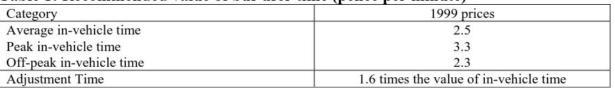
[image:12.595.86.528.660.726.2]Our recommended values for in-vehicle time are in set out in Table 1. While we have also found evidence of relationships between factors such as income and journey purpose and the value of time, it is not possible to make general recommendations on these aspects. Where appropriate local information should be used to adjust the recommended values. With regard to adjustment time valuation, there have been only a limited number of studies looking at this issue and these have been rail sector studies. As adjustment time is very closely linked to the concepts of “walk time” and “wait time” we have simply assumed that these values are the same magnitude.
Table 1: Recommended value of bus user time (pence per minute)
Category 1999 prices
Average in-vehicle time Peak in-vehicle time Off-peak in-vehicle time
2.5 3.3 2.3
Adjustment Time 1.6 times the value of in-vehicle time
We have reviewed the small number of studies that attempt to place a value on attributes of bus quality. These recommendations cme with a health warning, as they are largely based on two research studies. We have distinguished between London values and those from elsewhere which appear to be substantially lower.
Table 2: Values for Information Provision (1999 prices)
Information Type London Values Non-London Values
Real Time 9.7 pence per trip 5.2 pence per trip Printed Timetable 9.2 pence per trip 4.6 pence per trip
Table 2 shows recommended values for information provision but we also recommend a value of 2.5 pence per trip be used for the provision of pre-trip information (taking the value of standard timetables at home) for non-London based flows and 5 pence for London based flows. With regard to vehicle quality, we are largely distinguishing between a low floor vehicle and a non-low floor vehicle, we would recommend a value of a low floor vehicle of 2.5 pence per trip for London based passengers and 1.5 pence per trip for non-London based flows. Evidence from one study (SDG, 1996) suggests a total ceiling value to be placed on any package of measures of 26.1 pence for bus passengers in London, at this stage therefore we recommend the aggregation of quality attributes up to that value. Until contrary evidence is available we would suggest that the same payments ceiling be used but be adjusted for non-London passengers giving a total value of 13.5 pence.
(b) Determining sensitivity of Demand
The spread parameter θ1 governs the sensitivity of choice between services, whereas the
structural θ2 parameter represents the sensitivity to changes in the generalised cost of bus
as a whole. θ1 should be set to satisfy homogeneity and symmetry conditions (Henderson
and Quandt, 1958). Using the concept of conditional elasticity and a diversion factor, it is possible to determine the appropriate value for θ1, given an assumed operator specific
elasticity of demand with respect to changes in generalised cost of –4.0. Using this, the structural parameter θ2 can be estimated to give an overall elasticity of demand with
respect to fare of –0.4. Whist we have strong evidence on the overall short run market elasticity, evidence on operator specific or cross-elasticities between services is thin. We therefore recommend that this parameter be subject to sensitivity analysis.
4.3.4 Application of the Model to Forecast Demand
The way in which the model is applied is outlined below:
(i) For each OD pair on the network in a given operational period (e.g. a peak hour), we generate a sample of, say, 500 individuals with a given distribution of tastes (attribute values), characteristics (e.g. child, adult, pensioner) and most preferred departure times.
(iii) The market shares for each service and ticket type (for a given OD pair in a given operational period) are then estimated by averaging the derived probabilities over all 500 individuals.
(iv) The overall size of the bus market (total number of passengers for a given OD pair in a given operational period) is then determined in Level 2 of the model and subsequently assigned to individual services using market share estimates.
On this basis, total demand and revenue estimates can be derived for each service and ticket type. Where services are estimated to reach capacity, a “flag” is risen in the output to alert the analyst (we could alternatively set a maximum load factor and automatically increase service, through duplication, if required).
4.4 The Cost Model
The extant literature on cost models identifies three broad approaches to modelling cost information. The first is an engineering approach that attempts to allocate costs according to engineering relationships for wear and tear. The second is an econometric approach which uses statistical techniques such as regression to estimate costs as a function of output and input prices or alternatively to estimate output (or production) as a function of inputs. The final approach is the accountancy approach that attempts to allocate all costs to physical measures of output. Despite numerous shortcomings, this approach has been the dominant approach in public transport cost studies largely due to the need to process cost data for tax reasons. Ideally we would like to use an econometric model for bus costs but due to data availability we have had to rely on simpler accounting and average cost formulations.
4.4.1 Fully Allocated Costing Methods
The Chartered Institute of Public Finance and Accountancy (CIPFA) developed a fully allocated cost formula for the National Bus Company in 1974 (CIPFA, 1974). The formula attempts to allocate variable, semi-variable and fixed costs to measures of physical output, and identifies three measures of physical output to which costs can be allocated:
(i) Fuel, oil and tyre costs were allocated on the basis of distance operated, that is they were allocated according to vehicle kilometres (VKM);
(ii) Staff costs and vehicle maintenance costs were allocated on the basis of time operated, that is they were allocated according to vehicle hours (VH);
(iii) Vehicle depreciation and building costs were allocated according to peak vehicles (V).
An example of a fully allocated costing approach is given in Equation 4. As can be seen, total costs are a linear function of VH, VM and V, with average cost (in terms of vehicle miles) being inversely proportional to speed (VKM/VH) and vehicle utilisation (VKM/V) which is itself determined by the peakiness of the operation.
cV bVKM aVH
From DETR (2000) we have established that for an average vehicle in 1999, a=£16.41 per vehicle hour, b=£0.091 per vehicle km, and c=£15.16 per vehicle. To more accurately reflect costs it will be sensible to develop the model to reflect different vehicle types (mini, midi, single deck, double deck, low floor), different local operating conditions and different levels of quality (QBP and non-QBP traffic).
4.4.2 Passenger Infrastructure Costs
Passenger infrastructure costs can vary considerably across QBP types, a reflection of both the diversity of the road systems covered by QBP areas and the passenger infrastructure elements that are included in a QBP. Given this it is impossible to arrive at a universal average cost figure for QBPs, nor is it possible to report an average figure for similar types of QBPs (for example, those with high quality infrastructure), e.g. the average kilometre cost of the Line 33 QBP in Birmingham is around £150k, whilst in Edinburgh the cost per kilometre of Greenways is around £310k. What are therefore required are some detailed costs of specific attributes. At a recent QBP Conference organised by TAS (June, 2000), Clive Evans from CENTRO outlined some specific costs (2000 prices) associated with some QBPs:
• £8k to provide a Kassel kerb and paving at a bus stop;
• Driver training at £200 each;
• £6.2k for real time information at each bus stop; and
• £4.5 for a high specification QBP bus shelter.
Several issues can be raised about these costs the first of which is that, apart from driver training, they all fall on the local authority. This raises the question of whether to include them in the model since whilst they will not directly affect the bus operators’ costs they will impact upon the generalised cost of the passengers’ trips via those passengers’ valuation of quality attributes and the higher the number of passengers per bus, the slower the service and the higher the cost. The second issue that has to be determined is what the relative cost of passenger infrastructure provided for a QBP is compared with a non-QBP route. That is to say would bus shelters be provided on non-QBP routes and if so how much less do they cost as compared with a high specification QBP bus shelter. At the moment our preferred position would be to use the cost of passenger infrastructure as an input into a cost benefit analysis rather than as a model input. This issue also highlights the need to take into consideration the costs of any road infrastructure, such as bus lane and bus priority measures. Again none of these costs are allocated to the bus operators, yet the bus operators benefit via the quality of service bestowed upon their passengers together with any cost savings arising from improved vehicle speeds. At the moment we would recommend that these costs be treated like passenger infrastructure costs, in that they be assessed in a cost benefit framework alongside the outputs of the model. To do this it is necessary that any additional road infrastructure costs that are attributable to a QBP be identified.
4.4.3 Cost Conclusions
area being examined. Within the simulation model, we have allowed for the user to specify costs based upon the CIPFA formula or simply on a pence per kilometre basis. These costs are operator specific.
4.5 Evaluation Model
The evaluation model is based on the concept of economic welfare. In its simplest form this is taken as the unweighted sum of producer surplus and consumer surplus. Producer surplus (PS) is taken as revenue minus costs and consumer surplus (CS) is taken as the benefit individuals receive from consuming a good or service over and above its price. As such CS is taken to be a measure of user benefit and is defined by the shape of the demand curve and the price of the good or service in question. Since its introduction in the London Transportation Study (phase III, Tressider et al, 1968) the rule of a half has been widely used to determine user benefits. This rule is a simple formula that assumes the demand curve approximates a straight line over the relevant area of change, with the result that consumer surplus can be measured by way of the formula shown in equation 5.
ΔCS= 1 GCB −GCA VB +V
2( )( A) (5)
Where:
CS
Δ = the change in consumer surplus V = volume of travel
GC = generalised cost of travel
A and B = after and before situation respectively
Following Williams (1977) it is possible to estimate consumer surplus by direct integration of the demand curve but as we are dealing with marginal changes the rule-of-half provides a good approximation to this measure.
As yet, we have not taken into consideration other external benefits and costs in the evaluation framework. With regard to the environmental, decongestion and accident saving benefits that may arise from a mode switch from car to bus, we recommend that a lump sum benefit for each additional passenger is derived somewhat similar to that used by the (shadow) Strategic Rail Authority for evaluation purposed. Here a reduction in road vehicle miles brought about by a mode switch to rail is assumed to generate external benefits of £0.32 per reduced vehicle mile (OPRAF, 1999).
5. COMPETITIVE RESPONSE AND DYNAMICS
The model outlined in Section 4 produces a ‘snap shot’ of company profits (revenue minus costs) under different operating assumptions. The model is run for key operating periods and then grossed-up to generate weekly or annual estimates. Three different ways of applying the model can be envisaged.
• Optimisation. A different approach would be to define objectives for the operators and optimise the objectives subject to a set of constraints. Where competition is based on output, a Cournot or von Stackleberg equilibrium may arise (see Dodgson et al 1993 and Savage 1985 respectively); alternatively, where competition centres on price, a Bertrand equilibrium may arise (see James 1996).
• Generalisation. The third approach is a hybrid approach. It involves specifying, perhaps, 1000 scenarios and running the model in batch mode for each scenario. Simple regression models could then be estimated on the output. This would allow us to develop general demand, revenue and profit functions for each firm.
In each instance explicit behavioural response and decision rules should be used to assess where entry is feasible and sustainable.
6. DATA INPUTS
To operationalise the model, four sets of inputs are required:
(i) Information is needed to define the existing bus network, including timetable and fares information for each origin-destination movement and distances between stops. (ii) Information is needed to define parameters for both the demand and cost models.
Where local information in not available the default parameter estimates set out in Bristow and Shires (2001) and this document could be used.
(iii) Information on existing base demand for each OD movement is needed. Whilst the model will generate market shares and identify growth or contraction in the bus market, base demand information is needed to help determine absolute numbers of passengers and hence operator revenues.
(iv) The last piece of information required is a set of bus market share information varying by journey distance. This information is needed when applying the upper nest of the model to help determine how much the bus market can grow. Ideally this will vary by distance since for journey lengths under 0.5 km walk and cycle would tend to have the greatest market shares, whilst for journeys between 5-6 kms car and bus are the dominant modes. In the absence of more accurate local information, theses figure can be estimated from information contained in Table 3.3 of Transport Statistics Bulletin NTS: 1997/1999 Update (DETR, 2000). The figures in this table are subsequently adjusted to take account of non-travel.
7. A CASE STUDY – MODEL VALIDATION
The model was initially validated on simulated data for a hypothetical bus route. However, more recently, we have been able to validate the model on real data. The next section of the report provides a description of the case study and this is followed by a description of a series of model runs for looking at the introduction of quality and subsequent entry into the market by a second operator. It is intended that this case study is viewed as a demonstration of some of the capabilities of the model, rather than an in-depth analysis of the potential for QBPs.
Briefly, the route is 18.5km long incorporating 25 bus stops. The route is currently supplied by a single operator for most of its length, who operates a more or less uniform frequency of 4 buses per hour, between 6am and 6pm. The services are essentially inter-urban commuter services serving the outlying regions of a mid-sized British city. Within the city limits, the service faces on street competition. The data supplied shows the daily (6am to 6pm) demand for services from Monday to Friday in late July 1999 at approximately 1170 passengers. If all passengers pay full fare (i.e. assume that the difference between concessionary and full fares is made up by the local authority) and the average fare on the route is £1.09, the incumbent generates base daily revenue of £1280.40. There are a total of 1628 bus kilometres in the timetable and if each is costed at an average of £0.79, then we estimate total costs at £1286.12 and daily profits of £-6.20. For this time period, the incumbent is shown to more or less breakeven on this route, though we suspect that late July is not a typical operating period and that increased profits will be made at other times in the year. That said, we believe that this is a solid base to examine the impact of QBP.
7.2 Modelled Scenarios
We have chosen to look at the impacts of the introduction of a QBP using a scenario-based approach. In the first instance we look at the impact of a QBP on a monopoly supplier and assess whether the investment can be justified on increased revenues or whether a wider social cost benefit analysis in needed to justify investment. Following this, we use the model to look at the impact of new market entry and assess the likelihood of alternative competitive strategies based on fares, service levels and service quality.
7.2.1 How does a QBP impact on the monopoly supplier?
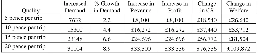
[image:18.595.77.507.661.752.2]Table 3 shows the annual demand and revenue implications of an increase in service quality for a monopoly operator. Quality enhancements valued at 5 pence per trip (say the provision of real time information) leads to a 2.2% increase in demand and a corresponding increase in revenue of £8,100. Assuming that the QBP has no cost or capacity implications for the operator, profitability is set to rise by £8,100 annually. Not surprisingly, consumers benefit from the increase in quality, with their net gain valued at £18,540 annually. Combining both operator profitability and consumer surplus gives a measure of benefit to society as a whole - excluding the capital and operating costs of the QBP investment, this benefit is valued at £26,640 annually. Additional model runs have been made for more significant increases in quality and these results are shown in Table 3 also.
Table 3: Demand implications of a QBP for a monopolist
Quality
Increased Demand
% Growth in Demand
Increase in Revenue
Increase in Profit
Change in CS
Change in Welfare
5 pence per trip 7632 2.2 £8,100 £8,100 £18,540 £26,640
10 pence per trip 15300 4.4 £16,272 £16,272 £37,440 £53,712
15 pence per trip 23148 6.6 £24,696 £24,696 £56,772 £81,504 20 pence per trip 31104 8.9 £33,300 £33,336 £76,536 £109,872
As well as improving bus quality, improvements to journey times and frequencies could also be assessed using this model together with complications such as second round effects on capacity requirement and demand levels. It is therefore quite easy to see how this model could be used to assess investment possibilities in a single operator case.
7.2.2 A Framework for Assessing Competition
If the increase in demand brought about though the introduction of a QBP is sufficient to trigger new entry into the market, then we need a methodological framework to be used to assess competition. The most pragmatic way forward is to specify a series of plausible competitive scenarios rather than define a set of supply side algorithms that lead model convergence at an equilibrium. The competitive strategies available to each agent include those based on: pricing, quantity, service quality and cost reduction. The costs and benefits associated with each scenario are then compared with base statistics for operator profitability, consumer surplus and overall economic welfare. The following sections detail possible strategies available to the Entrant and Incumbent, though the model is capable of assessing scenarios with many more operators.
(a) Price Strategies
The main pricing strategies of interest are those that may be pursued by the Entrant and the Incumbent. It is therefore assumed that the strategies of other operators, remain unchanged. In shorthand, the outcome of alternative price strategies is summarised as Price[Entrant, Incumbent], with price defined in relation to current incumbent fare levels as:
• Same – unchanged P[S,S];
• 10% Discount for all ticket types P[D10,S];
• 20% Discount for all ticket types P[D20,S]; and
• 30% Discount for all ticket types P[D30,S].
It is feasible that the entrant will price at the same level as the incumbent or discount in the short run to gain market share. Low prices may compensate for an inferior quality service, where the entrant is not part of the QBP scheme.
(b) Frequency (Quantity) Scenarios
As in determining appropriate pricing strategies, the main frequency strategies of interest are those that may be pursued by the Entrant and the Incumbent. Frequency, or output, scenarios are denoted in a similar way to pricing strategies and can be assigned as:
• Same - 4 buses per hour F[S,S];
• Low 3 - 3 buses per hour F[L3,S];
• Low 2 - 2 buses per hour F[L3,S]; and
• Low 1 - 1 buses per hour F[L1,S].
other hand is unlikely to wish to concede market share to the Entrant and will either maintain its existing service pattern or increase it in order to squeeze the Entrant’s profitability. Indeed, the Incumbent may take pre-emptive action to try and deter entry by filling any gaps in the timetable.
(c) Quality (QBP)
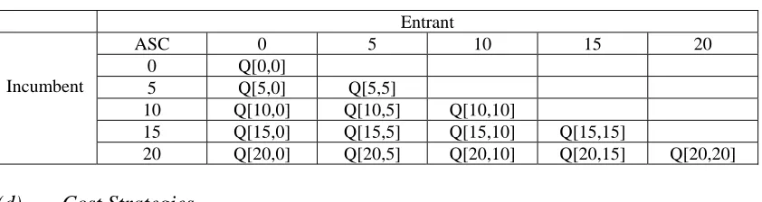
[image:20.595.87.508.303.415.2]All non-price, non-frequency attributes of operators can be summarised in terms of the Alternative Specific Constant (ASC). As these attributes are “unknown” we have made the decision to specify the ASC at five levels 0, 5, 10, 15 and 20 pence per trip. Quality attributes have been combined to show both operators participating in a QBP with various level of quality (the diagonal elements in Table 4) and to show the entrant either not participating in the scheme or only providing a limited improvement in quality (the lower triangle in Table 4).
Table 4: Quality Competition Matrix
Entrant ASC 0 5 10 15 20
0 Q[0,0]
5 Q[5,0] Q[5,5]
10 Q[10,0] Q[10,5] Q[10,10]
15 Q[15,0] Q[15,5] Q[15,10] Q[15,15]
Incumbent
20 Q[20,0] Q[20,5] Q[20,10] Q[20,15] Q[20,20]
(d) Cost Strategies
An alternative competitive strategy would be for the entrant to enter at low cost, e.g. using old buses and low cost labour). In this example we have assumed an overall cost reduction for the entrant of 10%.
(e) Combined Strategies
Although each competitive strategy can be pursued in isolation to each other, it is likely that operators will combine strategies to achieve the most favourable outcome. The combination of the 4 pricing strategies, 4 frequency strategies, 15 quality strategies and 2 cost strategies yields a total of 480 scenarios to be analysed. The presentation of this amount of data would be cumbersome and difficult to assess. To simplify analysis, the outcome of all tested scenarios have been analysed by a series of dummy variable regression runs.
Table 5 present the results of 3 dummy variable regression runs, with operator profitability and changes in consumer surplus and economic welfare taken as the dependent variables and the Incumbent’s and the Entrant’s strategies taken as the independent variables. Each model is calibrated on output data derived from the 485 simulation runs (480 combined strategies plus 4 monopoly strategies and the base).
The coefficients tell us what “on average behaviour of rivals” makes sense for each operator to do. This regression models can be used to locate areas of interest and general trends but reference should be made to individual scenario output where more detail is required.
Table 5: Regression Analysis on Operator Profitability, Consumer Surplus and Welfare - £ per day (t-stats shown in brackets)
Dep Variable
Variable
Incumbent Profit Model (a)
Change in CS Model (b)
Change in Welfare Model (c)
Constant -72.05 (4.9) 46.23 (3.2) 54.63 (4.2)
ASC 5 -Incumbent 58.25 (8.5) 39.13 (5.7) 61.80 (9.9) ASC 10 –Incumbent 119.03 (17.9) 78.86 (11.9) 124.82 (20.7) ASC 15 –Incumbent 181.35 (27.7) 119.76 (18.4) 189.50 (31.9) ASC 20 –Incumbent 245.15 (37.4) 162.03 (24.8) 256.32 (43.3) 10% Fares Discount -123.94 (30.9) 51.53 (12.9) 21.52 (5.9) 20% Fares Discount -254.48 (63.6) 119.44 (29.9) 35.45 (9.8) 30% Fares Discount -379.63 (94.9) 204.94 (51.5) 42.24 (11.7) 1 Service per hour -69.81 (4.8) -11.85 (0.8) -336.19 (25.5) 2 Service per hour -266.11 (18.4) 74.10 (5.2) -583.96 (44.4) 3 Service per hour -439.31 (30.3) 156.09 (10.8) -832.15 (63.2) 4 Service per hour -559.37 (38.6) 239.77 (16.6) -1066.99 (81.0) ASC 5 – Entrant -45.22 (11.7) 27.48 (7.1) 31.02 (8.8) ASC 10 – Entrant -91.72 (21.2) 56.34 (13.1) 63.76 (16.3) ASC 15 – Entrant -139.14 (27.6) 86.50 (17.3) 98.20 (21.6) ASC 20 – Entrant -187.51 (28.3) 117.97 (17.8) 134.32 (22.4)
Cost [0,-10%] na na 87.69 (34.3)
Adj R2 0.98467 0.95668 0.99141
Observations 485 485 485
Model (a) Incumbent Profitability
The constant shows a base daily operating loss of £72.05 for the incumbent operating without quality enhancements. Subsequent improvements in quality, valued at increments of five pence per trip, generate an increase in profitability of £58.25, £119.03, £181.35 and £245.15. Entry into the market by a second operator progressively reduces the incumbents profitability as the entrant’s service levels increase, fare levels reduce and quality improves, for example a new entrant operating 4 buses per hour, with a 30% fares discount and a high level of quality will reduce the incumbent’s profitability by around £1127 per day. This level of entry is not sustainable as it requires the entrant to absorb significant operating losses. From the incumbent’s perspective, an increased quality of service maintains a modest level of profitability even with some fringe competition, though it is likely that the incumbent would increase frequency to blockade entry.
Model (b) Change in Consumer Surplus
Model (b) shows the results of an increase in competition on the welfare of consumers. As would be expected, consumers benefit as quality is improved, service levels increased and fares reduced. It is interesting to examine the figures to see if alternative strategies other than quality enhancements can generate the same level of benefit to the consumer.
Model (c) Change in Welfare
profitability brought about as a result of entry. Here, welfare is taken to be the sum of profits from both operators together with consumer surplus. It is clear from this analysis that this route can not support two profitable operators unless the incumbent operator were to reduce its frequency or the overall size of the market were to grow significantly. The latter, of course, may happen at other times of the year.
Case Study Conclusions
The situation described assumes that both operators act independently of each other and that the cross elasticities of demand between services are high. In fact, if operators were to collude or the cross elasticities of demand are lower that assumed, the best strategy for each firm would be to price high and produce low. This strategy would be justified on the basis that the overall market elasticities on the route are low. Unless the market can grow significantly, or the incumbent reduce output levels, this route is unlikely to support two operators and although consumers would benefit from competition, society as a whole would suffer welfare losses.
8. SUMMARY AND CONCLUSIONS
The overall objective of this study was to develop a computer-based simulation model of the local bus market that can be used to assess the implications of a wide range of QBP initiatives.
As our starting point, we identified the characteristics that we would ideally like in a QBP model. These characteristics were defined by: the nature of the study objective, the range of situations to which the model could be applied (corridor based or network based), the quantity and quality of available data to use as inputs and the degree of flexibility needed so that the model could be adapted and improved.
Before beginning work on model development, we felt it prudent to review existing public transport models to see if we could adapt an existing model to suit the task in hand. This review covered strategic and semi-strategic models as well as operational models. Whilst none of the existing models could be used directly, we concluded that many of the ideas contained in the PRAISE and MUPPIT models would be of use to this project.
The structure of our preferred model contains three core elements, comprising: a demand model, a cost model, and an evaluation model. The demand model works at the individual level and assigns simulated passengers to operators, services and ticket types and allows for the overall size of the bus market to expand or contract according to the overall level of service. The cost model assigns total costs to operators using a CIPFA-type fully allocated costing formula, and the evaluation model estimates overall operator profitability, consumer surplus and a measure of economic welfare.
The QBP model has been embedded in a computer program which can be adapted by the analyst to examine a range of scenarios on corridor based network, the size of which can also easily be changed.
runs to help simplify analysis and produce some general relationships between operator profitability and the competitive strategies of operators.
REFERENCES
Bonsall, P. (1992) “Planning Land-Use and Transport Options”.
Bristow, A. and Shires, J. (2001) “A review of the values of time, elasticities of demand and other parameter values for use in the Quality Bus Partnerships model”, Report to the Department of the Environment, Transport and the Regions. February 2001.
Chartered Institute of Public Finance and Accountancy (1974) “Passenger Transport Operations” London.
Cooper, A. and Preston, J. (1993) “Urban Transport Market: Theoretical Analysis. Technical Note 3. MUPPIT – Model Development”. Institute for Transport Studies, University of Leeds.
DETR (1999a) “Focus on Public Transport”. The Stationery Office, London. Annex B. Tables 2, 15, 22 and 27.
DETR (1999b) “Transport Statistics Great Britain. 1999 Edition”. The Stationery Office London. Table 4.13.
DETR (2000) “Transport Statistics Great Britain. 2000 Edition”. The Stationery Office London.
Dodgson, J.S., Katsoulacos, Y. and Newton, C.R. (1993) “An Application of the Economic Modeling Approach to the Investigation of Predation”. Journal of Transport Economics and Policy 27 (2), 153-170.
ITS and Gibb Transport Planning (1998) “Working Paper 1: Theoretical Approach to Fares Competition Modelling” Consultancy report to Office of the Rail Regulator and the Office of Passenger rail Franchising.
Glaister, S. (Ed) (1987) "Can the Value of Transport Subsidy Be Measured", Transport UK, Policy Journals.
Grayling, T. and Glaister, S. (2000) “A New Fares Contract for London”. IPPR
Henderson, J and Quandt, R(1958) “Microeconomic Theory: A Mathematical Approach” , McGraw-Hill.
Hood, I. (1997) “MERLIN: Model to Evaluate Revenue and Loadings for Intercity”. PTRC, Summer Annual Meeting, Proceedings of Seminar H, Brunel University.
McClenahan, J.W., Nichols, D., Elms, M. and Bly, P.H. (1978) “Two Methods for Estimating the Crew Costs of Bus Services”. TRRL SR364.
MVA (1992) “Strategic and Regional Transport Model”, The MVA Consultancy. Woking, Surrey.
OPRAF (1999) “Planning Criteria – A guide to the Appraisal of Support for Passenger Rail Services” Office of Passenger Rail Franchising 1999.
Preston, J (1991) Explaining Competitive Practices in the Local Bus Industry: The British Experience” Transportation Planning and Technology, 15, 277-294.
Preston, J., Nash, C.A. and Toner, J. (1993) “MUPPIT: Urban Transport Market Theoretical Analysis”. ITS Working Paper 412.
Preston, J., Whelan, G.A. and Wardman, M. (1999) “An Analysis of the Potential for On-track Competition in the British Passenger Rail Industry”. Journal of Transport Economics and Policy, 33: 77-94, Part 1.
Savage, I.P. (1985) “The Deregulation of Bus Services”. Gower, Aldershot.
Steer Davis Gleave (1996) “Bus Passenger Preferences” Report Prepared for London Transport Buses.
Travers Morgan , R. and Partners (1974) “Costing of Bus Operations – Final Report of the Bradford Bus Study”.
Tressider, J.O, Meyers, D.A. Burrell, J.E and Powell, T.J. (1968) “The London Transport Study: Methods and Techniques”. Proceedings of the Institute of Civil Engineers, Vol 39, pp433-465.
White, P (2000) “Bus tendering in London – a critique” Paper presented to a workshop “review of London’s Bus Contracting Regime”
White, P.R. and Turner, R. (1989) “Costing and Productivity for Different Vehicle Types – An Analytical Framework”. Presented to International Conference on Competition and Ownership of Bus and Coach Services. Thredbo, Australia.