Experiment and modelling of birefringent flows using commercial CFD code

promoting access to White Rose research papers

White Rose Research Online

Universities of Leeds, Sheffield and York

http://eprints.whiterose.ac.uk/

This is an author produced version of a paper published inInternational Journal of Heat and Fluid Flow.

White Rose Research Online URL for this paper: http://eprints.whiterose.ac.uk/9117/

Published paper

Tomlinson, R.A., Pugh, D. and Beck, S.B.M. (2006) Experiment and modelling of birefringent flows using commercial CFD code. International Journal of Heat and Fluid Flow, 27 (6). pp. 1054-1060.

Experiment and Modelling of Birefringent flows using

Commercial CFD code

R.A. Tomlinson, D. Pugh, and S.B.M. Beck

Department of Mechanical Engineering,

The University of Sheffield, Mappin Street, Sheffield, S1 3JD, UK.

Keywords: Birefringent flows, Computer modelling, Experiments, Shear rate

Abstract

It is well known that certain fluids are birefringent and when flows are viewed in polarised

light interference fringes are observed. The fringes are caused by a phase shift in the light

passing through the fluid and are proportional to the integral of the maximum shear strains

in the fluid. In order to understand what is happening within the flow and overcome the

difficulties due to this integration of analysing three dimensional flows, additional

computational or experimental information is needed.

In this work, a commercially available computer code (Fluent) is used for the first time to

model the flows. The flow data are then exported to a spreadsheet where the shear rates are

integrated across the field and then banded for graphical output. The results from this are

then compared to results generated from birefringent flow experiments and the agreement is

found to be good since the modelled fringes show the same patterns as those in the

experiment. This novel use of computational and experimental techniques together will

Currently, there are still a lot of empirical variables involved in fitting the computational

fringes to the experiment, but the results of this preliminary study show that this is a

promising approach to this type of problem.

1. Introduction

The photoelastic effect is that property of transparent materials which causes them to

become birefringent or doubly refracting when deformed. In their free state, materials such

as glass, plastics and fluids are isotropic to the passage of light; light traversing them is

affected only by the normal elementary laws of optics. When deformed however, these

materials behave like most transparent crystals, in that they have distinct optical axes and

transmit light with different velocities along the planes of principal strain. When a ray of

light passes through a birefringent material under strain, it is split into two components

appropriate to the principal strains at any point; each ray then passes through the material at

a velocity which is proportional to the magnitude of the principal strain with which it is

associated, i.e. the material behaves as if it has two refractive indices, hence the term

birefringent. When the light exiting the material is viewed through a polarizing plate,

interference fringes can be observed. These fringes are caused by the phase shift in the light

that has passed through the material and are proportional to the maximum shear strain in the

material. Using birefringence to study strain in solid materials is well established and is

termed photoelasticity. The practical use of birefringence effects in fluids is still in its

infancy but it has already been used by Sun et al. (1999) for examining blood flow in

models of cardiovascular systems. As polymer melts are themselves birefringent, this is one

Maxwell (1872) and Mach (1873) first observed the phenomenon of flow birefringence

in the 1870’s. Early investigations into flow birefringence centred mainly on finding a

suitable fluid that could be used and which would produce sufficient fringes. Quantitative

studies of flow birefringence did not begin until the 1950’s. Theories produced to explain

the phenomena of flow birefringence have centred mainly around two areas:

1) stretching and orientation of long chain polymers.

2) deformation or orientation of suspended macromolecules or colloidal particles.

The fluids tested as part of this research fall into the second of these categories. Until the

work of Rosenberg (1952) the accepted theory was that birefringence in fluids was due to

the orientation of the molecules, but then he suggested that the birefringent effect was due

to deformation of the molecules rather than their orientation. This implies that the

interference fringes are related to the maximum shear stress in the fluid, τmax, and not the

streamlines as previously assumed. Therefore the effect is governed by the stress optical

law which can be found in Dally and Riley (1991)[:

cd Nλ

τ_max =

2 (1)

where N is the order of the fringe observed, c is the stress optical constant, d is the length of

the light path in the fluid and λ is the wavelength of the light.

This phenomenon therefore only occurs in birefringent fluids which are subject to shear

magnitude of these shear stresses. This means that as the stress varies within the fluid, the

optical phase difference also changes. So the total birefringent effect along the light path is

clearly the integral of the magnitude and direction of the shear stresses of the fluid,

τ

      = dy du

µ

τ

where

µ

direction.

This fact is particularly important for real, three dimensional flow, because a shear occurs at

the walls giving additional fringes due to the integrating effect. A review of integrated

birefringence in both solids and fluids up to 1998 can be found in Cen et al. (1998). In order

to understand what is happening within the flow and overcome this integrating effect, either

additional experimental or computational techniques must be used augment the information

available. Aben and Puro (1997) have investigated the use of optical tomography for 3-D

flow, but this method is intensive both in terms of storage and processing requirements.

Laser Doppler Anemometry (LDA) techniques have been used in conjunction with

birefringence to analyse two and three dimensional flows in non-Newtonian fluids by

Davidson et al. (1993). The same pair of techniques were used by Subramanian and Picot

(1996) to determine the stress optical coefficient using a convergent channel. Their flows

were slow, and thus the non-Newtonian effects were very pronounced.

Various workers have use a variety of methods to model and validate birefringence. These

tend to be made more difficult by the fact that most birefringent fluids tend to be

experimental finite element method to simulate these flows. The looked at instabilities in

lid driven cavities. However, they ignored the third dimension in this work. The pompom

method is a recent technique used to model 3-D fluid flow in polymer melts. The extended

form was used by Verbeeten et al. (2004) to model this type of birefringent flow, but the

authors’ main concerns were related to the convergence of the solution. Clemuer et al.

(2004) used the double converted form along with a Mueller Matrix method to describe the

birefringent effect to allow comparison of their results with experiment.

A different approach to the modelling was published by Li et al. (2000) who used their own

computational fluid dynamics (CFD) techniques to model and validate birefringence results.

Other work by the group incorporates shear thinning, and is mostly concerned with the

rheology of the flow.

The objective of the current research was to develop an alternative, simpler method for

modelling the birefringent effect. It uses a commercial CFD code (Fluent) and converts

flow fields into shear fields by post processing using a spreadsheet. By summing these

calculated shears, it is possible to compare these results to experimental ones. Two different

types of flows were investigated, an expanding circular jet and a cavity. The former gave a

three dimensional shear flow in the direction of the light and the latter was designed to give

a two dimensional effect. This use of a well validated CFD code means that future research

2. Experimental Work

2.1 Optical Apparatus

All the experiments in this investigation used a circular polariscope (Figure 1). The light

source was capable of producing both white and monochromatic light and was placed

behind a frosted glass screen to diffuse the light and ensure the light intensity was uniform

over the full field, reducing the glare. The light passed through the first polariser and a

quarter wave plate, then through the flow channel under investigation, through a second

quarter wave plate, and polariser (known as the analyser). The birefringent effect of the

fluid was captured using a digital video camera from which individual frames could be

acquired for analysis. The entire apparatus was surrounded by blackout curtains to remove

the background light. This not only made the fringes easier to see but also prevented

reflections from the waveplates that would cause the camera problems in focusing. Details

on photoelastic analysis can be found in the excellent book by Dally and Riley (1991).

2.2 Expanding Circular Jet

When a relatively fast moving flow of fluid in a small pipe enters a larger volume, it forms

a jet and there is high shear between the fast and slow moving fluids. This, along with a

certain amount of entrainment, causes the flow to slow down and expand. This flow

phenomenon is known as an expanding jet. It was decided to use this for the initial

birefringent flow experiments as the high shear rates involved would maximise the fringes.

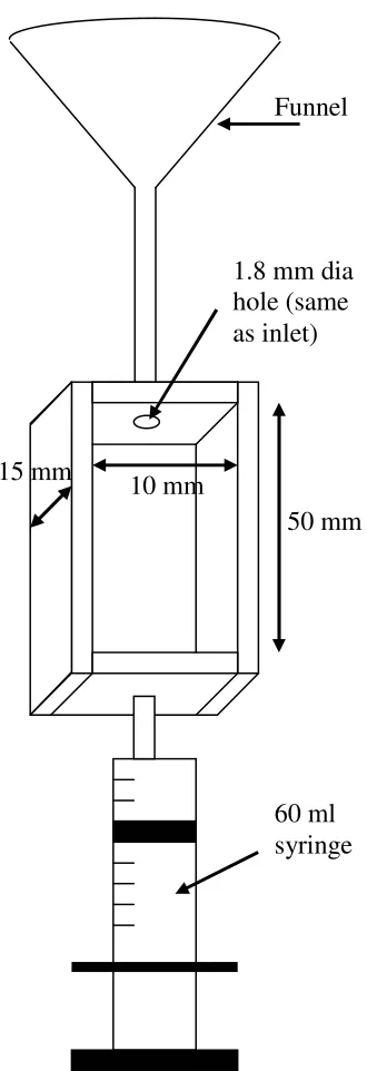
The flow channel for the expanding jet consisted of a 10ml syringe which forced the fluid

through a 1.8 mm circular hole into a 10 mm by 15 mm rectangular channel 50 mm long.

(Figure 2) . The channel was constructed of a PMMA frame with two glass walls through

which the fluid could be viewed (see Figure 1). The glass was of negligible integrated

birefringence and therefore did not affect the observed effects from the fluid. The channel

was positioned between the two quarter waveplates and was orientated so the syringe forced

the fluid vertically upwards. The camera was focused so that the entire channel was visible.

Since part of the syringe was in the frame of the camera, the flow rate of the fluid could be

calculated by taking the volume change over a number of frames, each of 0.04 s duration.

The fluid chosen for the experiment was hydroxypropyl cellulose (HPC) at 12%

concentration by weight. When the fluid was propelled into the channel, it expanded rapidly

in the form of a circular jet. This caused flow separation and high shear stresses within the

fluid and images of the birefringent effect were recorded in both light and dark field

arrangements, as shown in Figure 3.

The rate at which the syringe needed to be depressed to produce good fringe patterns was

very rapid and hence the fringes were only visible for about six frames (approximately 0.25

seconds). This made the accurate calculation of the velocity of the fluid difficult, but it was

approximately 10 ms-1. The rapid depression rate also meant that in the dark field

arrangement the light intensity suddenly increased and then decreased, reducing the quality

of the pictures. The solution also had small air bubbles forced into it by the high flow rate,

and the solution needed to be left to settle between runs to remove these. Ideally the fluid

would be continuously pumped, but due to the viscosity of the fluid, a positive

displacement pump would be needed and was not available.

Strong fringe patterns were observed in the expanding jet and in the case of the dark field

the order of the fringes for comparison with the computational model. Although the jet

experiment produced strong fringe patterns, the analysis of these fringes alone is difficult as

the nature of the flow is three-dimensional and the fringes that are seen are due to the

integral of the shear stresses through the sample. Hence the images in Figure 3 do not look

like a classical jet but have a bifurcated appearance. The perceived difference between the

expected and actual fringe pattern is a possible reason why commercial CFD codes have not

been used previously in this field.

The concentration of the HPC was lowered in 1% increments to 6%. Here fringes were still

visible but of lower order than before. The maximum fringe order observed varied with the

concentration of the solution reducing from a maximum of 1.5 fringes to 0.5 fringes with

the 12% and 6 % concentrations respectively. This observation may be explained by the fact

that the viscosity and therefore shear stress reduce with concentration, thus lowering the

fringe order.

2.3 Two-Dimensional Flow in a Cavity

A second channel was designed to approximate two-dimensional flow as shown in Figure 4.

This channel had a rectangular cross section with a large thickness to width ratio which

ensured that the path of the light would be relatively long without the volume of the channel

becoming too large. This was important, as the length of the light path, d, directly affects

the number of fringes produced (see equation (1)). A backward facing step was included in

the channel to produce the high shear stresses. The fluid was forced into the channel from a

60 ml syringe with a short length of copper pipe inserted into the end of it, via 6 mm tubing

into a 75 mm long duct 3 mm high and 18 mm thick. This allowed the velocity profile to

into a chamber 50 mm long. The duct then reduced back to the same dimensions as the inlet

and another 6 mm tube was used at the outlet. This tube led to a vertical funnel which was

used both as a reservoir and a filling mechanism. The sudden expansion of the fluid after

the step caused flow separation and hence high shear stresses in the fluid. The shear stresses

and thus the fringes in the birefringent fluid occurred directly after the step, so the camera

was focussed on this area.

This channel was also constructed with glass walls either side which were held in place by

grooves in a PMMA frame. The end sections of the channel were secured by the use of

screws. This channel was placed between the two quarter waveplates (Figure 1) so that the

glass sides were parallel to them. The syringe was clamped vertically with the outlet facing

downwards which helped to prevent air bubbles entering the channel during the

experiments as the air in the syringe would automatically rise to the top.

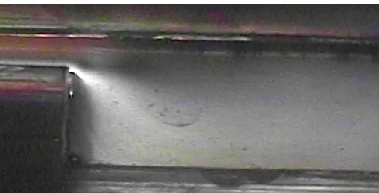
The initial experiments for flow in the cavity used a 12% concentration of HPC. This was

then reduced in 1% increments down to 7% (Figure 5 shows the fringes observed in the

channel with a concentration of 7%). For each concentration the flow rate and image of the

birefringent fringes were recorded. The flow rate was calculated by recording on the

soundtrack of the video camera when the fluid had reached certain levels. High

concentrations of HPC, with high fluid viscosity, produced low fluid flow rates and could

only be timed over 5-20ml. Once the concentration reached 7%, the viscosity had dropped

sufficiently for the fluid to be timed over the entire 60 cc volume of the syringe.

It had been expected that due to the higher flow rates at lower viscosities, the fringe order

expanding jet. However it was noticed that the fringe order was increasing rather than

decreasing. The HPC was diluted further in increments of 0.5% down to 4%.

3. Computational Modelling

All the modelling work to produce the velocity fields used the CFD package FLUENT4.

The computational grid models were created in Pre-BFC and after convergence, velocity

components were imported into a spreadsheet. The velocity boundary conditions and fluid

properties were obtained from the experimental work described above. Once in the

spreadsheet the velocities were transformed from u, v and w components into velocity

magnitudes using Pythagoras’ theorem.

The shear stress, τ, at each point requires the differential of the velocity magnitude and

these were found for every node using upwind differencing in the z direction (in the

direction of the light path - see Figure 4) It is appreciated that any method of producing the

partial differentials could be used.

1 1 − − − − ≈ ∂ ∂ i i i i y y u u y u (3)

where i is the element and i-1 is the previous element with respect to the light path.

A two dimensional projection of these results was produced by summing these results in the

z direction which gave values proportional to the optical phase shifts. A surface plot of

these was produced, and when correctly banded, could be compared with the experimental

To make the CFD calculations easier, the fluid was treated as Newtonian. It was also

assumed that flow birefringence obeys the stress optic law, equation (1) and that indices of

refraction that are related to the shear stress are the sole cause of the birefringent effect.

3.1 Modelling of Expanding Jet

The domain for the model of the expanding jet was 20×60×12 cells. In order to reduce the

computational time, only one quarter of the channel was modelled and symmetry cells were

used in both directions perpendicular to the flow. To increase the information in the inlet,

the concentration of cells was doubled in the inlet half of the channel so that there were 40

cells were in the first half and only 20 in the second half.

Two flow situations were modelled, using 6% and 12% solutions of HPC. As can be seen in

Figure 6, after processing the data, the 6% solution gave a good agreement with the

experimental observations. In this figure, the experimental and computational data are

shown as mirror images on either side of the centre line with the flow going from left to

right. The 12% solution of HPC however produced inferior results, as the modelled fringes

produced did not appear to spread out at the entrance to the channel. This was thought to be

due to the non-Newtonian nature of the fluid as was borne out from the experimental

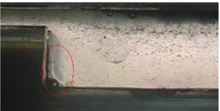
observations that fringes were “frozen” into the fluid at the end of the step experiments.

Although probably present at higher concentrations, this effect was first noticed at 10%

concentration. At the base of the step, a permanent fringe was observed after drawing the

fluid into the syringe (Figure 7). Very faint fringes were also noticed after experiments

where stronger fringes had been present during flow. Unfortunately these fringes were too

faint for the camera to pick up. These stress frozen fringes indicate that the solution is

non-Newtonian feature of the fluid1. An additional issue of this non-Newtonian flow was that

the Reynolds number was not entirely correct. The initial assumption for the computational

model was that the fluid was Newtonian with a viscosity measured at a relatively low rate

of shear. The actual viscosity was lower than this value, as shown in Figure 8. It was

therefore decided to repeat the computational model with the viscosity lowered from

1.6 kg m-1 s-1 to 0.74 kg m-1 s-1. At this value, the fringe pattern of the jet was seen to

bifurcate as observed during the experiments (Figure 9). This value was used for all the

analysis using 12% HPC solutions. As the computational model is seen to agree well with

the experimental results, this implies that the approach taken to process the results is an

acceptable one for these preliminary studies.

3.2 Modelling of the Cavity

The grid for the cavity consisted of 100×11×13 cells. As the channel had a single line of

symmetry down the centre in the direction of flow this was mimicked in the computational

grid by placing a surface of symmetry cells in the centre of the channel. This helped to

reduce the computation time as well as the amount of data that needed processing. To

improve the data produced by FLUENT4 the number of cells was increased for the

expansion, and also in the inlet duct to ensure the flow was fully developed. Care needed to

be taken at this stage as weighting of the cells incorrectly could give poor results and cause

problems in the analysis. Refinement of the grid was considered in the z direction around

1

Establishing the non-Newtonian stress deformation law for this fluid was a task beyond

the centre of the channel for the inlet and outlet but this was not done, as it would have

caused difficulties with the differencing due to the variation in the grid size.

The computation was carried out with 5% and 10% concentrations of HPC. Once again, a

correction was made to account for the effective viscosity for the higher concentration. The

fringe patterns have been banded to approximate the fringes observed experimentally and

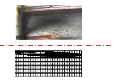
are shown, along with the equivalent experimental results in Figures 10 (5% concentration)

and 11 (10% concentration). The flow in this case goes from left to right. Although these

data are not as clear as those from the expanding jet, a close resemblance can be seen in the

fringe patterns. This figure shows that that the computational results can correctly predict

the area of greatest shear and hence highest fringe order.

This is particularly clear when one examines the first, white, fringe from the experiment. In

the case of the 5% concentration , the flow goes parallel to the top, and the maximum shear

occurs as the high speed jet goes over the step which is shown in Figure 10. The same

comparison can be applied to the 10% results, except in this case the areas go down from

the step at about 35° from horizontal. This is because the greater viscosity will cause the jet

to become attached to the wall.

4. Discussion

The aims of this work were to show that the birefringent analysis could be applied

successfully to fluid flow and that it was possible to use minor modifications of

commercially available CFD software to model the fields which had been produced

experimentally. In both of the geometries tested, the simple approach taken by the authors

It has been shown that after processing, the salient features of both the two and three

dimensional flow experiments can be identified and explained. This is particularly so in the

case of the expanding jet where the fringes do not actually appear as expected due to the

integral effect of the birefringence through the channel which gives the appearance of the

flow splitting into two jets. That the modelling shows the same effect, both supports the

validity of the modelling method and explains the experimental result.

Although the fringes at high concentrations are clearly visible, more fringes would be

desirable. As the flow rate is close to transition to turbulent, higher flow rates are

impossible as the linear birefringent effect only works in laminar flow; an increased cross

section of the flow channel would be a good method of achieving this.

The non-Newtonian nature of the fluid has been noted and to a certain extent accounted for

by linearising its value at the operating condition. From the data obtained using the

expanding jetand CFD, at a flow rate of 10 m s-1 and 12% concentrations the viscosity was

found to be out by a factor of two. To obtain more correct results, a full shear rate against

viscosity calibration of the fluid and also the use of the non-Newtonian flow model in

FLUENT would have to be implemented.

In this work, the contribution of the shear stresses lying in the plane of the light ray was

considered to be equal to that of the shear stresses perpendicular to it. This is unlikely

actually to be the case and investigation into this area should be considered.

Other methods of increasing the order of the fringes produced could be examined for

further investigations. Alternative solvents for HPC could be used to improve the fringes as

the fringe order. These work by reflecting the light back through the channel a number of

times, increasing the path length of the light.

It is fully appreciated that the work shown here is still in its early stages. For example, the

viscosity and fringe constants required to make the experiment and theory agree have to be

chosen by the operator. Undoubtedly these could be selected on a more rigorous basis. The

fluid should also be optically calibrated to enable the bands to be automatically selected.

Finally, it would be relatively straightforward to implement both the non-Newtonian flow

and shear rate calculations directly within the latest versions of many CFD packages,

making processing the results a far easier task.

5. Conclusions

This work has shown that the use of hydroxypropyl cellulose (HPC) in investigating flow

birefringence produces results that can lead to quantitative analysis of the flow fields. It also

illustrates that increased flow rates have a marked effect on the fringe order.

The cavity experiments combined with CFD of the same geometry show that calibration of

the fringe data from HPC is possible. The agreement between the experimental and

computational results illustrates that what is happening in the flow is understood, making

the two-dimensional calibration possible.

The expanding jetused has demonstrated that three dimensional analysis of flow using flow

birefringence is possible even though the results from the experiment may not appear to

show an expanding jet. In this case computational analysis can be also used to calibrate the

fluid optically. To analyse this form of flow from the birefringence results, more work is

These results present a simple way forward in the modelling of birefringent flows as

standard CFD codes can be used to extract flow fields which can then easily be integrated

and scaled. Overall the method shows great promise and, as it is a full field method where

time varying flow phenomena can be analysed, it will provide a valuable element in the

fluid mechanic’s toolbox.

References

Aben, H., and Puro, A., 1997, Photoelastic tomography for three-dimensional flow birefringence studies, Inverse Problems, 13, 215-221.

Cen, M., Hickman, L.J, Tomlinson, R.A., and Patterson, E.A., 1998, Integrated birefringence applied to solids and fluids - a review, Proceedings of 11th International Conference on Experimental Mechanics, Oxford, August 1998, 507-512.

Clemeur, N., Rutgers, R.P.G., and Debbaut, B., 2004, Numerical evaluation of three-dimensional effects in planar flow birefringence, Journal of Non-Newtonian Fluid Mechanics, 123, 105-120.

Dally, J.W., and Riley, W.F., 1991, Experimental Stress Analysis, McGraw-Hill, Inc.

Davidson, D.L, Graessley, W.W., and Schowalter, W.R., 1993, Velocity and stress fields of polymeric liquids flowing in a periodically constricted channel. 1. Experimental methods and straight channel validations, Journal of Non-Newtonian Fluid Mechanics, 49, (2-3), 317-344.

Grillet, A.M., Shaqfeh, E.S.G , and Khomami, B., 2000, Observations of elastic instabilities in lid-driven cavity flow, 94, 15-35.

Li, J.M., Burghardt, W.R., Yang, B., 2000, and Khomami, B, Birefringence and

computational studies of a polystyrene Boger fluid in axisymmetric stagnation flow, Journal of Non-Newtonian Fluid Mechanics, 91, (2-3), 189-220.

Mach, E., 1873, Optische-akustische Versuche, Clava, Prague.

Martyn, M.T., Groves, D.J., and Coates, P.D., 2000, In process measurement of apparent extensional viscosity of low density polyethylene melts using flow visualisation, Plastics Rubber and Composites, 29, (1), 14-22.

Maxwell, J.C., 1872, Double Refraction of Viscous Fluid Motion, Proc. Roy. Soc.,(London), A22, 46.

Rosenberg, B., 1952, Navy Dept., David W. Taylor Model Basin Report No. 617.

Subramanian, R., and Picot, J.J.C., 1996, A rheo-optical analysis of converging wedge flow for estimation of stress-optical coefficient, Polymer Engineering and Science, 36, (9), 1196-1202.

Sun, Y.D., Sun, Y.F., Sun, Y., Xu, X.Y., Collins, M.W., 1999, Visualisation of dynamic flow birefringence of cardiovascular models, Optics and Laser Technology, 31, 103-112.

Figure 1. Experimental arrangement of the circular polariscope where: L = Light source; P = Polariser; Q = Quarter wave plate; A = Analyser

P

Q

Flow channel

_{Digital video}

camera

1.8 mm dia hole (same as inlet)

50 mm 10 mm

15 mm

60 ml syringe Funnel

a) _b)

Figure 3. Showing the birefringent fringes due to the 12% HPC acting as an expanding

25 150

75

50 8

Light path through the thickness (18 mm) of the channel

3 Outlet

3 Inlet ₁₈

Figure 4. Cross sectional diagram of the cavity.

Figure 5. Showing the fringe pattern observed the cavity using 7% concentration of HPC in a

Figure 6. Experimental and Computational fringe patterns from the expanding jet experiment

using 6% HPC

Newtonian

Plastic

Reduced Viscosity

Point at which viscosity readings were taken

Shear rate du/dy

S

h

ea

r

st

re

ss

τ

Figure 8. Expected (Newtonian) and real (Plastic) relationship

Figure 10. Banded FLUENT4 Data used to Predict Fringe Patterns for 5% HPC and

Experimental Results for 5% HPC

Area of

Figure 11. Banded FLUENT4 Data used to Predict Fringe Patterns for 10% HPC

Area of