Solar cycle influence on the interaction of the solar wind with Local Interstellar Cloud

This is a repository copy of

Solar cycle influence on the interaction of the solar wind with

Local Interstellar Cloud

.

White Rose Research Online URL for this paper:

http://eprints.whiterose.ac.uk/1717/

Article:

Izmodenov, V.I., Malama, Y. and Ruderman, M.S. (2005) Solar cycle influence on the

interaction of the solar wind with Local Interstellar Cloud. Astronomy and Astrophysics, 429

(3). pp. 1069-1080. ISSN 1432-0746

https://doi.org/10.1051/0004-6361:20041348

[email protected] https://eprints.whiterose.ac.uk/ Reuse

Unless indicated otherwise, fulltext items are protected by copyright with all rights reserved. The copyright exception in section 29 of the Copyright, Designs and Patents Act 1988 allows the making of a single copy solely for the purpose of non-commercial research or private study within the limits of fair dealing. The publisher or other rights-holder may allow further reproduction and re-use of this version - refer to the White Rose Research Online record for this item. Where records identify the publisher as the copyright holder, users can verify any specific terms of use on the publisher’s website.

Takedown

If you consider content in White Rose Research Online to be in breach of UK law, please notify us by

DOI: 10.1051/0004-6361:20041348

c

ESO 2005

Astrophysics

&

Solar cycle influence on the interaction of the solar

wind with Local Interstellar Cloud

⋆

V. Izmodenov

, Y. Malama

, and M. S. Ruderman

1 _{Lomonosov Moscow State University, Department of Aeromechanics and Gas Dynamics,}

Faculty of Mechanics and Mathematics, and Institute of Mechanics, Moscow 119899, Russia e-mail:[email protected]

2 _{Institute for Problems in Mechanics, Russian Academy of Sciences, Prospect Vernadskogo 101-1, Moscow 117526, Russia} 3 _{Department of Applied Mathematics, University of Sheffield, Hicks Building, Hounsfield Road, Sheffield S3 7RH, UK}

Received 25 May 2004/Accepted 3 September 2004

Abstract. We present results of a new time-dependent kinetic model of the H atom penetration through the solar wind – interstellar medium interaction region. A kinetic 6D (time, two dimensions in space, and three dimensions in velocity-space) equation for interstellar H atoms was solved self-consistently with time-dependent Euler equations for the solar wind and interstellar charged components. We study the response of the interaction region to 11-year solar cycle variations of the solar wind dynamic pressure. It is shown that the termination shock location varies within±7 AU, the heliopause variation is∼4 AU, and the bow shock variation is negligible. At large heliocentric distances, the solar cycle induces 10–12% fluctuations in the number density of both primary and secondary interstellar H atoms and atoms created in the inner heliosheath. We underline the kinetic behavior of the fluctuations of the H atom populations. Closer to the Sun the fluctuations increase up to 30–35% at 5 AU due to solar cycle variation of the charge exchange rate. Solar cycle variations of interstellar H atoms in the heliospheric interface and within the heliosphere may have major importance for the interpretation of H atom observations inside the heliosphere.

Key words.Sun: solar wind – interplanetary medium – ISM : atoms – Sun: activity – hydrodynamics

1. Introduction

More than 30 years (three solar cycles) of solar wind observa-tions show that its momentum flux varies by factor of∼2 from solar maximum to solar minimum (Gazis 1996; Richardson 1997). It was shown theoretically that such variations of the so-lar wind momentum flux strongly influence the structure of the heliospheric interface – the region of the solar wind interaction with the local interstellar medium (e.g., Karmesin et al. 1995; Wang & Belcher 1998, 1999; Baranov & Zaitsev 1998; Zank 1999; Zaitsev & Izmodenov 2001; Scherer & Fahr 2003a,b; Zank & Mueller 2003; Izmodenov & Malama 2004a,b).

Most global models studying the solar cycle effects ignore the interstellar H atom component or took this component into account by using simplified fluid (Scherer & Fahr 2003a,b) or multi-fluid (Zank & Mueller 2003) approximations. These sim-plifications were done because it is difficult to solve 6D (time, two dimensions in space, and three dimensions in velocity-space) kinetic equation for the interstellar H atom component. A kinetic description of interstellar atoms is necessary due to their large mean free path comparable with the size of the he-liospheric interface. Recently, it has been shown explicitly by Izmodenov (2001), Izmodenov et al. (2001) that the velocity

⋆ _{Appendix is only available in electronic form at}

http://www.edpsciences.org

distribution function of interstellar atoms is not Maxwellian. Fluid or multi-fluid approaches assume the velocity distribution of H atoms to be Maxwellian or the sum of several Maxwellian distributions. This assumption introduces additional uncertain-ties in the model. (To estimate these uncertainuncertain-ties one needs to compare a multi-fluid model with a kinetic model for each spe-cific set of model parameters.) Consequently, the multi-fluid approaches adopted for H atoms in the heliospheric interface may result in misleading interpretations of observational data. At the same time, the momentum flux variations of the solar wind may have a significant effect on the distribution of inter-stellar H atoms in the heliosphere due to coupling of the atom and plasma components by charge exchange. Therefore, it is necessary to study solar cycle effects by solving 6D kinetic equation self-consistently with fluid plasma equations. In this paper we present the results of such a model.

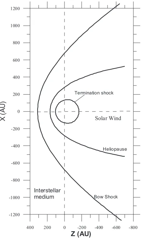
The qualitative pattern of the heliospheric interface is shown in Fig. 1. The solar wind plasma decelerates and turns to the tail at the termination shock (TS), while the interstellar plasma decelerates and turns outward of the axis of symmetry at the bow shock (BS). The heliopause (HP), which is a con-tact discontinuity, separates these two plasma flows. Hydrogen atoms newly created by charge exchange have the velocities of their ion partners in the charge exchange collisions. Therefore, the parameters of these new atoms depend on the local plasma

400 200 0 -200 -400 -600 -800

Z (AU)

-1200 -1000 -800 -600 -400 -200 0 200 400 600 800 1000 1200

X(

A

U

)

Termination shock

Solar Wind

Heliopause

Bow Shock

Interstellar medium

Fig. 1.Structure of the heliospheric interface, the region of the inter-action of the solar wind and the Local Interstellar Cloud.

properties. It is convenient to distinguish four different popu-lations of H atoms: 1) atoms created in the supersonic solar wind; 2) atoms originating in the heliosheath and known as he-liospheric ENAs (Gruntman et al. 2001); 3) atoms created in the disturbed interstellar wind; 4) original (or primary) inter-stellar atoms.

2. Model

In this work we advance the heliospheric interface model developed by the Moscow group (e.g. Baranov & Malama 1993; Izmodenov et al. 1999; Alexashov et al. 2000, 2004a,b; Myasnikov et al. 2000; Zaitsev & Izmodenov 2001; Izmodenov & Alexashov 2003; Izmodenov et al. 2003a,b; Izmodenov et al. 2004; for reviews see Izmodenov 2003, 2004) by introducing 11 year sinusoidal variations of the solar wind in the model. The goal of this paper is to exploretheoreticalaspects of non-stationary interaction of the solar wind and the local interstellar cloud. The results presented here cannot be directly applied to interpretation of observational data.

We consider all the plasma components (electrons, protons, pickup ions, solar wind alpha particles and interstellar He ions)

as one fluid with total densityρand bulk velocityu_{. It is} as-sumed that all ionized components have the same tempera-tureT. Although this assumption cannot be made in the case of the solar wind, the one-fluid model is based on mass, mo-mentum and energy conservation laws and predicts the plasma bulk velocity and locations of the shocks very well.

The plasma is quasi-neutral; i.e.,ne =np+nHe+ for

inter-stellar plasma, andne = np+2nHe++ for the solar wind. The

interstellar and interplanetary magnetic fields are ignored in the paper. Protons interact with H atoms by charge exchange. While the interaction of interstellar H atoms with protons by charge exchange is important, for helium ions the process of charge exchange is negligible because of small cross sections for the charge exchange of helium atoms. Hydrodynamic equa-tions for the charged component are solved self-consistently with the kinetic equation for the H atom component.

The governing equations for the charged component are the following:

∂ρ

∂t +∇ ·(ρu)=q1,

∂(ρu)

∂t +∇ ·(ρuu+pI)=q2, (1)

∂E

∂t +∇ ·[(E+p)u]=q3.

Hereρis the total density of the ionized component, pis the total pressure of the ionized component,E = ρ(ε+u2/2) is the total energy per unit volume, ε = p[(γ₋1)ρ]−1 _{is the} specific internal energy, andI is the unit tensor. The temper-ature of the plasma is determined from the equation of state

p=2(np+nHe+)kT for the interstellar plasma andp=(2n_p+

3nHe++)kT for the solar wind, wherekis Boltzman’s constant;

np,nHe+ andn_He++ are the proton, interstellar He ion and solar

wind alpha particle number densities. In addition to Eqs. (1) we solve the continuity equation for He+_{in the interstellar medium}

and forα-particles in the solar wind. Then the proton number density is calculated asnp =(ρ−mHenHe)/mp, wherenHe de-notes the He+ number density in the interstellar medium, and the He++number density in the solar wind.

The right hand parts,q1, q2 andq3, are sources of mass, momentum and energy due to charge exchange of H atoms and protons, photoionization and electron impact ionization (Baranov & Malama 1993):

q1 =mHnH(νph+νimp),

q2 =mH uσHPex(u)(wH−wp)fH(wH)

×fp(wp) dwHdwp

+mH

(νph+νimp)wHfH(wH) dwH, (2)

q3 =mH

νph+νimp

w

2 H

2 fH(wH) dwH

+mH uσHPex(u) w2

H−w 2 p 2

×fH(wH)fp(wp) dwpdwH.

Here, u = _|w_{p −} w_{H| is the relative atom-proton velocity,} σHP

with a proton;νphis the photoionization rate;mHis the atomic mass; νimp is the electron impact ionization rate. Numerical values for σHPex, νph and νimp are given in Izmodenov et al. (1999) and Izmodenov et al. (2004). The function fp(wp) =

np(√πcp)−3exp(−(wp−u)2/c2p) is the local Maxwellian veloc-ity distribution function of protons, with the parameters (np, u,cp = (2kT/mH)1/2) determined by the solution of the Euler Eqs. (1). The function fH(wH) is the velocity distribution func-tion of H atoms.

The velocity distribution of H atoms fH(r,wH,t) is calcu-lated from the linear kinetic equation:

∂fH

∂t +wH·

∂fH

∂r +

F mH·

∂fH ∂w_H =₋fH

|w_H−w_p|σHPex fp(r,wp) dwp (3)

+ fp(r,wH)

|w∗_H−w_H|σHPex fH(r,w∗H) dw∗H

−(νph+νimp)fH(r,wH).

Here w_{p and} w_{H are the individual proton and H atom} ve-locities, respectively, and F is the sum of the solar gravita-tional force and the solar radiation pressure force. The plasma and neutral components interact mainly by charge exchange. Photoionization, solar gravity and radiation pressure taken into account in Eq. (3) are only important at small heliocentric dis-tances. Electron impact ionization may be important in the inner heliosheath, which is the region between the termina-tion shock and the heliopause. Note that photoionizatermina-tion rate and solar radiation pressure may vary with the solar cycle. At present we do not include solar cycle variations of these param-eters in our model, but we plan to do so in the future.

The boundary conditions for Euler equations are the fol-lowing. We assume that the solar wind is spherically symmetric at the Earth orbit. It makes our model axissymmetric. We also assume that, at the Earth orbit, the solar wind number density oscillates harmonically, while the bulk velocity and tempera-ture remain constant:

npE =npE,0(1+δnsinωt),

vE =vpE,0, (4)

TE =TE0=const.

For the solar wind disturbances determined by Eq. (4), the ratio of the maximum to minimum momentum flux is equal to∆ = (1+δn)/(1−δn). Following Baranov & Zaitsev (1998) we made

calculations for δn = 1/3, so that∆ = 2. As it was pointed

out by Zank & Mueller (2003), the solar cycle effects in the heliospheric interface remain the same when the variation of the solar wind dynamic pressure is caused by the solar wind velocity variation. In this paper we consider variations of the solar wind density which is sufficient for the purposes of this paper. The effects of the realistic solar cycle on the TS variation were studied by Izmodenov et al. (2003a).

The following solar wind parameters averaged over a few solar cycles were used:npE,0 = 8 cm−3,VpE,0 = 445 km s−1. We also used the following parameters of the interstellar gas in the unperturbed interstellar medium at the outer boundary:

VLIC = 26.4 km s−1, TLIC = 6500 K, nH,LIC = 0.18 cm−3,

np,LIC = 0.06 cm−3. These particular values of the interstellar velocity and temperature were chosen on the basis of the re-cent observations of the interstellar He atoms by GAS/Ulysses (Witte et al. 1996; Witte 2004; Gloeckler et al. 2004). The choice of nH,LIC and np,LIC is based on our analysis of the Ulysses pickup ion measurements (see, e.g., Izmodenov et al. 2003a,b, 2004).

Now we explain why we assumed “idealized” harmonic perturbations at the Earth orbit rather than the realistic pertur-bations of the solar wind parameters obtained from observa-tions. The statistical Monte-Carlo method used to obtain pe-riodic solutions of the kinetic equation requires us to fix the time-period. The non-linear nature of the system may lead to the interaction of the external 11-year fluctuations with the in-ternal oscillations of the heliospheric interface. As a result, os-cillations with periods different from 11 years may appear in the self-consistent solution of the governing Eqs. (1)−(3) with the boundary conditions (4). One of the main objectives of our study was to verify if such oscillations do appear. To do this we increased the time-period of our Monte-Carlo calculations by 6 times. If oscillations with periods different from 11 years are present in our solution we would be able to determine these periods. If we use the realistic perturbations of the solar wind parameters that are, in general, not periodic, as the boundary conditions, it would be rather difficult to detect the presence of oscillations with periods different from 11 years.

To solve the Euler equations self-consistently with the ki-netic equation we used as iterative procedure as suggested by Baranov et al. (1991) for the stationary model. In the first step of this iterative procedure the Euler equations with the con-stant source termsq1,q2andq3were solved with the use of the boundary conditions (4). The source terms were taken from the stationary solution with the average solar wind parameters. We performed calculations over 300 solar cycles. As a result, we got the distribution of the plasma parameters. We analyzed this distribution and found that there is the 11 year periodicity only. In the second step we solved the kinetic equation by a Monte Carlo method with splitting of trajectories (Malama 1991). To increase the statistical efficiency of the method, we assumed periodicity with the time periodtperiod=66 years. To minimize statistical errors we averaged the statistical results over tmc = 1 year. When doing so we used a distribution of the plasma parameters for the last 66 years obtained in the first step. As a result, we obtained the periodic (66 year)q1,

q2 andq3 source terms. In the third step we solved the Euler equations with the boundary conditions (4) and the periodic source terms obtained in the second step. Again, we performed gas dynamic calculations over 300 solar cycles. Analysis of the plasma distributions shows the 11 year periodicity only. Then we solved the kinetic equation by the Monte Carlo method with the distribution of the plasma parameters for the last 66 years obtained in the third step. We continued this process of iteration until the results of two subsequent iterations were practically the same.

solutions of this system of equations may exist. These solu-tions may have periods different from 11 years. The numerical method used to solve Euler equations does not need any re-stricting assumptions. Remarkably, as it is reported in the next section, our numerical solution does not contain oscillations with periods different from 11 years.

In addition to the “ideal” solar cycle calculations we carried out some complimentary calculations. We increased the solar wind ram pressure by a factor of 1.5 during the first 11 years of our 66-year period (Fig. 2, bottom plot). This study was in-spired by the fact that observations of the solar wind are re-stricted to the recent∼30 years. We wanted to understand how the solar wind conditions in the past, when they were not ob-served, influence the heliospheric interface and observational quantities at present and in the future.

3. Results

3.1. Plasma component

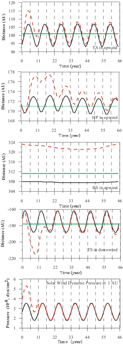
The variations of the heliocentric distances to the termination shock, heliopause and the bow shock are shown in Fig. 2. The discontinuities vary with a 11-year time-period under the ac-tion of 11-year fluctuaac-tions of the solar wind dynamic pressure at the inner boundary of our computational grid. The termi-nation shock oscillates from its minimal distance of∼93 AU, which is reached in the last (11th) year of the “ideal” solar cy-cle, to its maximum distance of ∼107 AU, which is reached during the fourth year of the cycle. Fluctuations of the TS are bigger in the downwind direction than in the upwind direction. By the upwind direction we mean the direction that is opposite to the direction of the Sun-LIC relative motion. The downwind direction coincides with the Sun-LIC velocity vector. The vari-ation of the TS in the downwind direction is∼25 AU from its minimum value of∼163 AU during the third year of the cy-cle to its maximum value of∼188 AU in the 9th year of the cycle. In the upwind direction the most distant position of the termination shock is reached∼1.5-year after the maximum of the solar wind dynamic pressure at 1 AU. The variations of the solar wind dynamic pressure are shown at the bottom of Fig. 2 for convenience. The phase of downwind fluctuations of the TS is shifted by∼3.5 years compared the phase of the up-wind fluctuations. It is interesting to compare our results with the results obtained by Zank & Mueller (2003) and Scherer & Fahr (2003a,b) on the basis of (multi-) fluid descriptions of the interstellar H atoms (Table 1).

The strength of the TS has important consequences for spectra of anomalous cosmic rays (ACRs) because the velocity jump at the TS is related to the spectral index of ACRsβthat determines the variation of intensity of the cosmic rays jwith energyE: j_∼ Eβ_{. We have computed the variation of the}

ve-locity jump at the TS. In the upwind direction the jump of the plasma velocity at the TS, or, in other words, the strength of the TS, varies from its minimum value of 2.92 to its maximum value of 3.09. This corresponds to the variation ofβfrom 1.28 to 1.22. The strength of the TS varies from 2.92 to 3.17 in the downwind region. This strength variation is translated into the variation ofβfrom 1.28 to 1.19.

0 11 22 33 44 55 66

90 95 100 105 110 115 120

Di

s

ta

n

c

e

(AU

)

TS in upwind

0 11 22 33 44 55 66

-220 -200 -180 -160

Di

s

ta

n

c

e

(AU

)

TS in downwind

0 11 22 33 44 55 66

168 170 172 174 176 178

Di

s

ta

n

c

e

(A

U)

HP in upwind

0 11 22 33 44 55 66

304 308 312 316 320 324

D

is

ta

n

ce

(AU)

BS in upwind

0 11 22 33 44 55 66

1 2 3 4 5 6

P

res

su

r

e

(1

0

-8,d

y

n

/c

m

2) _{Solar Wind Dynamic Pressure at 1 AU}

Fig. 2.Time variations of the heliocentric distances to the termination shock, bow shock and the heliopause in the upwind direction, and to the termination shock in the downwind direction. Bottom plot shows variations of the solar wind momentum flux,ρEVE2, with time. Dashed

Table 1.Results of calculations.

Model ∆SWa _{∆TS (upwind)}b _{∆TS (downwind) ∆HP (upwind) R(BS)}

time−R(BS)cstationary

This paper 2 14 AU 25 AU 4 AU 3 AU

Zank & Muller (2003) 2 7 AU 50 AU 6 AU n/a

Scherer & Fahr (2003) 2.67d

∼16 AU n/ae _{n/a >15 AU}

a_{∆SWnotes the ratio of maximum to minimum the solar wind dynamic pressure.} b_{∆ =R}

max−Rminis the difference between maximum and minimum distances of the TS, HP and BS during the solar cycle. c_R(BS)

time−R(BS)stationaryis the difference between mean location of the BS during the time-dependent calculations and the stationary solution. d_{Model “Sin 800” in Fig. 4a in Scherer & Fahr (2003b).}

e_{n/a means that we were unable to find the corresponding value from the results presented in the cited paper.}

The heliopause fluctuates with smaller amplitude as com-pared to the termination shock. It varies from 169 AU, which is reached during 4th year of the solar cycle, to 173 AU reached in the 9th year of the solar cycle. The distance to the heliopause averaged over the solar cycle is∼171 AU. This coincides with the stationary solution. The solar-cycle induced fluctuations of the BS is less than 0.1 AU in the upwind direction. The fluctu-ations are not visible in Fig. 2. The distance to the BS averaged over the solar cycle is∼308 AU, while this distance is∼311 AU in the case of the stationary solution.

Dashed curves in Fig. 2 correspond to solution of the prob-lem with the “broken” first of six solar cycles, when we in-creased the solar wind ram pressure by a factor of 1.5 during the first 11 years of our 66-year periodic calculations (bottom plot in Fig. 2). The termination shock in the upwind direction “feels” the increase of the solar wind dynamic pressure dur-ing approximately 4−5 years after the increase ended. In the downwind direction the “feeling” is somewhat longer and lasts another solar cycle. The second maximum of the TS both in the upwind direction (dashed curve on the top plot in Fig. 2) and in the downwind direction is closer to the Sun compared to the subsequent maxima.

The post-reaction of the heliopause to the 50% increase of the solar wind dynamic pressure is much longer compared to the reaction of the termination shock. The heliopause does not return to its periodic fluctuations even at the end of the 66-year time-period. One can see from the figures that the heliocentric distances to the termination shock, heliopause and bow shock are always larger in the case of a “broken” solar cycle compared to our “regular” solar cycles. This is related to the fact that the solar wind ram pressure averaged over 66 years is 8% greater compared to the “regular” cycle calculations. The effect is the most pronounced for the bow shock. It appears that 66 years are not enough for the BS to relax to its “regular”-cycle position. As a result, the BS is ∼10 AU away for the “broken”-cycle calculations compared to the “regular” cycle.

Plasma parameters undergo 11-year fluctuations in the entire computation region. However, the wave-length of the plasma fluctuations in the solar wind is apparently larger com-pared to the distances to the TS and HP. This means that time snap-shots of the distributions of plasma parameters (den-sity, velocity and temperature) are not qualitatively different from stationary solutions. The situation is different in the outer heliosheath, which is the region between the HP and BS. 11-year periodic motion of the heliopause produces a number

of additional weak shocks and rarefaction waves (Baranov & Zaitsev 1995). The amplitudes of these shocks and rarefaction waves decrease while they propagate away from the Sun due to the increase of their surface areas, interaction between the shocks and rarefaction waves, and the dissipative attenuation of the shocks. To resolve the wave structure we increased the res-olution of our computational grid by three times in the region. We have checked also that an additional increase of the res-olution of our computational grid does not change the results. Figure 3 presents distributions of plasma density, velocity, pres-sure and temperature as functions of the heliocentric distance in the upwind direction at two different moments (t1 =1 year (curves 1) andt2=6 year (curves 2). It is seen that the charac-teristic wavelength in the region is∼40 AU. Long-scale waves are also seen in plasma distributions in the post-shocked plasma of the downwind region (Fig. 3, left column). Amplitudes of the waves are much less than in the upwind direction and the wavelength is_∼200 AU.

Figure 3 shows a comparison of the 11 year average dis-tributions of interstellar plasma parameters (dots) with those obtained from stationary solution. The stationary calculations were performed with exactly the same inner and outer bound-ary conditions as used in the time-dependent calculations. At the Earth’s orbit we assume 11 year average values of the so-lar wind density. It is seen that the two distributions practically coincide. The congruence with the stationary solution is ad-ditional evidence of sufficient resolution of our computational grid and the lack of significant numerical dissipation in our numerical calculations. Our results contradict the conclusion made by Zank & Müller (2003) that “the shocks provide addi-tional heating in the heliotail and outer heliosheath”. According to our results the heating is very small and it is not notice-able in our calculations. However to draw conclusion on the plasma heating in the heliosheath, Zank & Müller (2003) had compared their time-dependent results with a stationary model that assumed smaller solar wind dynamic pressure compared with the 11-year averaged value. Therefore, the observed heat-ing could be 1) due to the shock heatheat-ing; 2) due to different boundary conditions. Additional multi-fluid study is needed to distinguish between these two mechanisms.

160 200 240 280 320 -16 -12 -8 -4 0 4 Ve lo c it y (k m /s )

160 200 240 280 320

0.1 0.12 0.14 0.16 P rot on num be r de ns it y (c m -3)

160 200 240 280 320

Distance (in AU) 1 2 3 4 5 P las m a T e m p er at u re (1 0 4,K

) _{160 200 240 280 320}

4 8 12 16 20 24 P re ss u re (1 0 -1 3dy m /c m 2) 2 2 2 2

-700 -600 -500 -400 -300 -200 -100 -140 -120 -100 -80 -60 -40 V elo c ity (k m /s )

-700 -600 -500 -400 -300 -200 -100 0.001 0.002 0.003 0.004 0.005 P rot on n um b e r de n si ty (c m -3)

-700 -600 -500 -400 -300 -200 -100

Distance (in AU) 0 5 10 15 20 25 P las m a T em p e rat u re (1 0 5,K

) -700 -600 -500 -400 -300 -200 -100

3 4 5 6 7 8 P re s su re (1 0 -1 3dy m /c m 2) UPWIND DOWNWIND

Fig. 3.Interstellar plasma number density, velocity, pressure and temperature as functions of the heliocentric distance for two different moments of time:t1=1 year (curves 1),t2=6 year (curves 2). Stationary solution (curves 3) and averaged over 11 years time-dependent solution (dots) are shown.

comparison to the characteristic scale of inhomogeneity. The latter assumption enabled us to use the WKB approximation. In addition, we neglected the interaction of the plasma pertur-bations with the H atoms. Then, using the reductive perturba-tion method, we derived the governing equaperturba-tion for the plasma perturbations. This equation is a generalization of the nonlin-ear equation used in nonlinnonlin-ear acoustics for the description of sound waves. We solved this equation assuming the boundary conditions at the heliopause corresponding to the harmonic os-cillation of the heliopause with period of 11 years and ampli-tude of 2 AU. Our main result is that, due to the nonlinear steep-ening, the shock forms in the wave profile at about the middle of the distance between the heliopause and the bow shock. The wave energy dissipation in this shock causes strong attenua-tion of the perturbaattenua-tions in their way from the heliopause to the bow shock. As a result, the wave amplitude at the bow shock

is about 3 times smaller than that predicted by the linear the-ory. Since the wave energy flux is proportional to the amplitude squared, this implies that almost 90% of the wave energy is dis-sipated in the shocks. On the basis of this result we conclude that the main reason why the solar cycle variation almost does not disturb the bow shock is that the perturbations propagating from the heliopause to the bow shock are strongly attenuated due to dissipation in the shocks.

Comparison with numerical results reveals that the attenua-tion of the perturbaattenua-tions obtained in the numerical simulaattenua-tion is even stronger than that predicted by the analytical solution. The most probable cause of this difference is that the interaction be-tween the plasma perturbations and the H atoms provides an additional wave dissipation.

0 100 200 300 400 500 R (AU)

0 0.2 0.4 0.6 0.8 1 1.2 1.4

n

/n

L

IC

0 100 200 300 400 500

R (AU) 1E-005

1E-004 1E-003 1E-002 1E-001

n

/n

0 100 200 300 400 500

R (AU) -1.6

-1.4 -1.2 -1 -0.8 -0.6 -0.4 -0.2

0 100 200 300 400 500

-4 -2 0 2 4

V

2

/V

H,

L

IC

15 15.5 16 16.5 17 17.5

0 100 200 300 400 500

R (AU)

4000 8000 12000 16000 20000 24000 28000

T

, K

0 100 200 300 400 500

R (AU)

1E+004 1E+005 1E+006

T

,K

Primary interstellar atoms Secondary interstellar atoms

Secondary interstellar atoms

Primary interstellar atoms

Primary interstellar atoms Secondary interstellar atoms

Atoms created in the inner heliosheath

Atoms created in the inner heliosheath (left Y-axis)

Atoms created in the inner heliosheath Atoms created in the

supersonic solar wind

Atoms created in the supersonic solar wind (right Y-axis)

Atoms created in the supersonic solar wind

plasma heating due to wave dissipation. We found that the mean temperature of the plasma in the outer heliosheath can be increased by about 280 K during one solar cycle. The plasma heating due to the wave dissipation is compensated by the en-ergy loss due to convective plasma motion and due to the in-teraction between the plasma and the H atoms as seen from the results of our numerical calculations.

3.2. H atoms

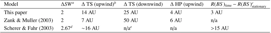
The main advantage of our model compared to previously published multi-fluid models (Scherer & Fahr 2003; Zank & Mueller 2003) is a rigorous kinetic description of the interstel-lar H atoms. Charge exchange significantly disturbs the inter-stellar atom flow penetrating the heliospheric interface. The atoms newly created by charge exchange have velocities of their ion partners in the charge exchange collisions. Therefore, the velocity distribution of these new atoms depends on the lo-cal plasma properties at the place of their origin. As it was dis-cussed in the introduction, it is convenient to distinguish four different populations of H atoms depending on the region in the heliospheric interface where the atoms originate. Figure 4 compares the distributions of the populations of H atoms ob-tained by the stationary model (dots) with the time-dependent solution averaged over 11 years. For the plasma component there is no noticeable difference between these two distribu-tions. Although we present only distributions in the upwind di-rection, our conclusion remains valid for all the computational domain. The stationary distributions of the H atom parameters for directions different from upwind could be found in our ear-lier papers (see, e.g., Izmodenov 2000; Izmodenov et al. 2001). To evaluate time-dependent features in the distribution of H atoms in the heliospheric interface we plot the number sities of the four populations of H atoms normalized to the den-sities obtained in the stationary solution. By doing this we sup-pressed spatial gradients of the densities, which are apparently larger than the time-variations of the densities. Figure 5 shows the normalized densities for two different years of the solar cy-cle. Solid curves correspond tot1 =1 year and dashed curves tot2 = 6 year. It is seen that the variation of the density is within ±5% of its mean value for the primary and secondary interstellar populations, and for the atoms created in the inner heliosheath. Closer to the Sun, for distances less than 10 AU, the amplitude of the fluctuations increases up to 15%. The vari-ation of the number density of H atoms created in the super-sonic solar wind is±30% about its mean value.

Figure 6 shows the time-variation of the number densities, bulk velocities and kinetic temperatures of three populations of H atoms at different heliocentric distances in the upwind direction. All parameters are normalized to their initial val-ues att =0. Clear 11-year periodicity is seen for the number densities of the atoms. Deviation from the exact 11-year pe-riodicity is related to the errors of our statistical calculations, which are ∼2−3%. Less than 10% variation (from maximum to minimum) is seen for number densities of all populations at distances greater than 10 AU. At 5 AU the variations are of the order of 30%. Variations of the bulk velocity and kinetic

0.92 0.96 1 1.04

0.92 0.96 1 1.04

0.92 0.96 1 1.04

0 100 200 300 400

Heliocentric Distance (AU)

0.6 0.8 1 1.2 1.4

Primary interstellar Atoms

Secondary interstellar atoms

Atoms created in the inner heliosheath

Atoms created in the supersonic solar wind

t1=1 year

t₁=1 year

t1=1 year

t1=1 year

t2=6 year

t2=6 year

t2=6 year

t2=6 year

Fig. 5.Time-variation of the number densities of primary and sec-ondary interstellar atoms (top panels), H atoms created in the inner heliosheath and H atoms created in the supersonic solar wind (bottom panels) as functions of heliocentric distance for two different moments in the solar cycle.

0.88 0.96 1.04 0 1 2 3 1 1.1 1.2 1.3

R=160 AU; upwind R=160 AU; upwind

R=160 AU; upwind

0 11 22 33 44 55 66

Time (year)

0.88 0.96 1.04

0 11 22 33 44 55 66

Time (year)

0.96 1.04 1.12

0 11 22 33 44 55 66

Time (year)

1 1.2 1.4

R=250 AU; upwind R=250 AU; upwind

R=250 AU; upwind

0.88 0.96 1.04 1.12 0.9 1 1.1 1.2 0.9 1 1.1 1.2 1.3

R=190 AU; upwind

R=190 AU; upwind R=190 AU; upwind

0.96 1 1.04 0.8 1.2 1.6 0.92 0.96 1 1.04

R=120 AU; upwind

R=120 AU; upwind

R=120 AU; upwind

0.96 1 1.04 1.08 1.12 0.8 0.88 0.96 1.04 0.9 1 1.1

R=90 AU; upwind

R=90 AU; upwind

R=90 AU; upwind

0.96 1 1.04 1.08 1.12 0.88 0.96 1.04 0.88 0.96 1.04

R=50 AU; upwind

R=50 AU; upwind

R=50 AU; upwind

0.88 0.96 1.04 0.92 0.96 1 1.04 0.88 0.92 0.96 1 1.04

R=15 AU; upwind R=15 AU; upwind R=15 AU; upwind

0.7 0.8 0.9 1 1.1 0.96 1.04 1.12 0.88 0.96 1.04

R=5 AU; upwind

R=5 AU; upwind R=5 AU; upwind

H a tom Density _{H a tom V elocity H atom Temperature}

0.8 1 1.2

R=160 AU; upwind

0 11 22 33 44 55 66

Time (year)

R=250 AU; upwind

0.8 0.9 1 1.1 1.2

R=190 AU; upwind

1 1.1 1.2

R=120 AU; upwind

0.8 1 1.2 1.4 1.6

R=90 AU; upwind

0.8 1.2 1.6

R=50 AU; upwind

0.6 0.8 1 1.2 1.4

R=15 AU; upwind

0.6 0.8 1 1.2 1.4

R=5 AU; upwind Pla sma Den sity

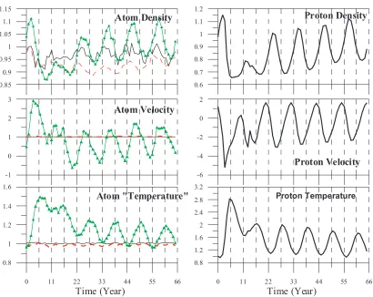
Fig. 6.The number densities (second column from the left), bulk velocities (second column from the right) and kinetic temperatures (right column) of the primary (solid curves) and secondary (dashed curves) interstellar atom populations and the atoms created in the inner heliosheath (curves with diamonds) at different heliocentric distances in the upwind direction as functions of time. For comparison, the number density of the plasma is shown (left column). All parameters are non-dimensionlized to their values att=0.

It is important to note that number densities of all three components of H atoms fluctuate in the same phase. Such co-herent behavior of fluctuations remains in the entire super-sonic solar wind region (R < 90 AU) for the three popula-tions of H atoms and in the inner heliosheath for the primary and secondary atoms. The reason for such coherent behavior of the variations of H atom densities becomes evident when we compare them with the plasma density variations (Fig. 6, left column). The two quantities vary almost in anti-phase. Apparently, such a correlation is only possible when temporal variations of the H atom densities are caused by variation of the local loss of the neutrals due to charge exchange and ionization

processes. The local fluctuations are not transported over large distances because the velocities of individual atoms are chaotic and their mean free path is large.

0.6 0.7 0.8 0.9 1 1.1 1.2

Proton Density

-6 -4 -2 0 2

0 11 22 33 44 55 66

Time (Year)

0.8 1.2 1.6 2 2.4 2.8 3.2 0.85

0.9 0.95 1 1.05 1.1 1.15

-1 0 1 2 3

0 11 22 33 44 55 66

Time (Year)

0.8 1 1.2 1.4 1.6

Atom Density

Atom Velocity

Atom "Temperature"

Proton Velocity

Proton Temperature

Fig. 7.Comparison of variations of density, velocity and kinetic temperature of H atoms created in the inner heliosheath (left column, lines with triangles) with those plasma parameters (right column). The variations are shown atR=160 AU in the vicinity of the heliopause in the upwind direction for “broken” solar cycle calculations, where we increase the solar wind ram pressure by factor of 1.5 during the first 11 years of chosen 66-year time-period.

secondary interstellar atom populations are in anti-phase with variations of primaries in the outer heliosheath (see, R = 190 AU in Fig. 6) and almost in phase with plasma fluctua-tions in the region. Again, the creation processes are dominant in the outer heliosheath for the population of the secondary in-terstellar atoms.

Finally, it is important to note that the behavior of the H atom populations in the heliospheric interface has kinetic nature. Variations of the atom parameters are determined by the loss and creation processes rather than by the convection and pressure gradient terms as it would be in the fluid de-scription. The fluid description is valid if the Knudsen num-ber Kn = l/L _≪ 1, wherelandLare the mean free path of the particles and the characteristic spatial scale of the problem, respectively. For the stationary problem the distance between the HP and BS, which is approximately 100 AU, can be chosen asL. The mean free path of H atoms in the region is_∼50 AU. Therefore, Knstationary ≈ 0.5. The results obtained on the ba-sis of the kinetic and fluid descriptions where compared by Baranov et al. (1998) and Izmodenov et al. (2001). This com-parison has shown explicitly that the velocity distribution func-tion of H atoms is non-Maxwellian everywhere in the interface. For the time-dependent problem considered in this paper the characteristic size,L, is determined as a half of the wavelength

of plasma fluctuations. In the region between the HP and BS

L_≈20 AU as follows from Fig. 3. Therefore, Kntime≈2 and a fluid description is even less appropriate than for the stationary model. The fact that the fluid description is inappropriate for the atom motion is the most probable cause of the big discrep-ancy between our results and the results obtained by Zank & Mueller (2003) and Scherer & Fahr (2003) who used the multi-fluid and multi-fluid approaches, respectively. It is interesting to note the qualitative difference between the Zank & Mueller (2003) and Scherer & Fahr (2003) results. The reason for this discrep-ancy could be once again the different description of H atoms used in these two papers. Scherer & Fahr (2003) used a one-fluid description for H atoms, while Zank & Mueller (2003) used a three-fluid description for H atoms in the interface.

4. Summary

Our basic results for the plasma component confirm the re-sults obtained previously:

1. The solar cycle variation of the TS location is±7 AU about its mean value.

2. The heliopause varies by±2 AU about its mean value. 3. The variation of the bow shock location is negligible. 4. There is a sequence of additional weak shocks and

rarefac-tion waves in the region between the heliopause and the bow shock. The additional heat of the plasma in the outer heliosheath induced by the shock waves is small and it is not observable in our calculations.

5. Our numerical results in the region between the HP and BS are confirmed by an analytical solution based on the WKB approximation.

For the interstellar H atom component we obtain the following new results:

1. Variation of the number density of the H atoms in the outer heliosphere is within 10%. The variation increases at 5 AU up to 30% due to strong ionization processes in the vicinity of the Sun.

2. The variations of the number densities of three populations of H atoms – primary and secondary interstellar atoms, and atoms created in the inner heliosheath – are coherent in the entire supersonic solar wind region and determined by loss due to charge exchange. The coherent behavior of fluctua-tions disappear in the regions where the production process is dominant.

3. There is no significant variation of the temperature and bulk velocity of the primary and secondary interstellar H atoms with the solar cycle. However, the bulk velocity and kinetic temperature of atoms created in the inner heliosheath vary with the solar cycle by 10–12%. It is shown that this varia-tion reflects the plasma properties at the heliopause. 4. There is a qualitative difference between our results and the

results obtained by using the fluid or multi-fluid description for the interstellar H atoms. It was shown that the multi-fluid description is less appropriate for the time-dependent case than for the stationary case because the Knudsen num-ber is larger for the time-dependent problem.

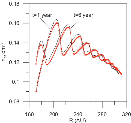
In addition, we have performed specific calculation of the time-dependent Euler equation with the source terms (3) taken from the corresponding stationary solution. The difference in plasma distribution with the self-consistent model is a few percent (Fig. 8). Therefore, we suggest that time-dependent multi-fluid models may produce results that are closer to the kinetic time-dependent model in the case when the source terms are taken from the stationary solution.

Acknowledgements. We thank Prof. A. I. Khisamutdinov for a fruitful discussion regarding periodicity of the global heliospheric interface structure and Monte Carlo methods. The calculations were performed by using the supercomputer of the Russian Academy of Sciences. This work was supported in part by INTAS Award 2001-0270, RFBR grants 04-02-16559, 04-01-00594, RFBR-NSFC grant 03-01-39004, NASA grant NNG04GB80G and International Space Science Institute

160 200 240 280 320

R (AU) 0.08

0.1 0.12 0.14 0.16 0.18

np

,c

m

-3

t=1 year t=6 year

Fig. 8.Comparison of the time-dependent self-consistent model re-sults (solid curves) with the solution of the time-dependent Euler equation with the source terms (3) taken from the corresponding sta-tionary solution (connected dotted). The figure presents the distribu-tion of plasma number density in the upwind direcdistribu-tion for two diff er-ent momer-ents of the solar cycle. The difference between two models is a few percent.

in Bern in the frame of the ISSI team “Physics and Gas Dynamics of the heliotail” “Determination of H atom parameters of the LIC from within the heliosphere (PI – E. Moebius)”.

References

Alexashov, D. B., Baranov, V. B., Barsky, E. V., & Myasnikov, A. V. 2000, Astron. Lett., 26, 743

Alexashov, D. B., Chalov, S. V., Myasnikov, A. V., Izmodenov, V. V., & Kallenbach, R. 2004a, A&A, 420, 729

Alexashov, D. B., Izmodenov, V. D. B., & Grzedzielski, S. 2004b, Adv. Spca Res., 34, 1, 109

Baranov, V. B., & Malama, Yu. G. 1993, J. Geophys. Res., 98, 15157 Baranov, V. B., & Malama, Yu. G. 1996, Space Sci. Rev., 78, 305 Baranov, V. B., & Zaitsev, N. A. 1998, Geophys. Res. Lett., 25, 4051 Baranov, V. B., Lebedev, M. G., & Malama, Yu. G. 1991, ApJ, 375,

347

Baranov, V. B., Izmodenov, V., & Malama, Yu. G. 1998, J. Geophys. Res., 103, A5, 9575

Gazis, P. R. 1996, Rev. Geophys., 34, 379

Gloeckler, G., Moebius, E., & Bzowski, M. 2004, A&A, in press Gruntman, M., Roelof, E., Mitchell, D., et al. 2001, J. Geophys. Res.,

106, 15767

Izmodenov, V. V. 2000, Astrophys. Space Sci., 274, issue 1/2, 55 Izmodenov, V. V. 2001, Space Sci. Rev., 97(1/4), 385

Izmodenov, V. V. 2004, in The Sun and the Heliosphere as an Integrated System, ed. G. Poletto, & S. T. Suess (Kluwer), in press Izmodenov, V. V. 2003, Proceedings of the Interstellar enviroment of the heliosphere, COSPAR Colloqium in Honour of Stanislaw Grzedzielski, ed. D. Breitschwerdt, & G. Haerendel, MPE Report, 285, 113

Izmodenov, V. V., & Malama, Y. G. 2004b, Proc. 3rd IGPP Conf. on Astrophysics – Physics of the Outer Heliosphere, Riverside, California, 8−13 February 2004, AIP, Conf. Proc., 719, 47 Izmodenov, V., Gruntman, M., & Malama, Yu. G. 2001, J. Geophys.

Res., 106, 10681

Izmodenov, V. V., Geiss, J., Lallement, R., et al. 1999, J. Geophys. Res., 104, 4731

Izmodenov, V., Gloeckler, G., & Malama, Yu. G. 2003a, Geophys. Res. Lett., 30, 1351

Izmodenov, V. V., Malama, Yu. G., Gloeckler, G., & Geiss, J. 2003b, ApJ, 954, L59

Izmodenov, V., Malama, Yu. G., Gloeckler, G., & Geiss, J. 2004, A&A, 414, L29

Karmesin, S. R., Liewer, P. C., & Brackbill, J. U. 1995, Geophys. Res. Lett., 22, 1153

Malama, Yu. G. 1991, Astrophys. Space Sci., 176, 21

Myasnikov, A., Alexashov, D., Izmodenov, V., & Chalov, S. 2000, J. Geophys. Res., 105, 5167

Narain, U., & Ulmschneider, P. 1990, Space. Sci. Rev., 54, 377

Priest, E. R. 1982, Solar Magnetohydrodynamics (Dordrecht: Reidel) Richardson, J. D. 1997, Geophys. Res. Lett., 24, 2889

Rudenko, O. V., & Soluyan, S. I. 1977, Theoretical Foundations of Nonlinear Acoustics (New York, London: Plenum Publishing Corporation, Consultant Bureau)

Scherer, K., & Fahr, H. J. 2003a, Geophys. Res. Lett., 30 Scherer, K., & Fahr, H. J. 2003b, Annales Geophys., 21, 1303 Wang, C., & Belcher, J. W. 1998, J. Geophys. Res., 103, 247 Wang, C., & Belcher, J. W. 1999, J. Geophys. Res., 104, 549 Witte, M., Banaszkiewicz, M., & Rosenbauer, H. 1996, Space Sci.

Rev., 78, 289

Witte, M. 2004, A&A, 426, 835

Zaitsev, N. A., & Izmodenov, V. V. 2001, in The Outer Heliosphere: The Next Frontiers, ed. K. Scherer, H. Fichtner, H. J. Fahr, & E. Marsch, 65

Zank, G. P. 1999, in Solar Wind 9, ed. S. Habbal, R. Esser, J. Hollweg, & P. Isenberg, AIP, 783

V. Izmodenov et al.: Solar cycle e ects on the heliospheric interface,Online Material p 2

x

R

Sun

heliopause

bow shock

0

m

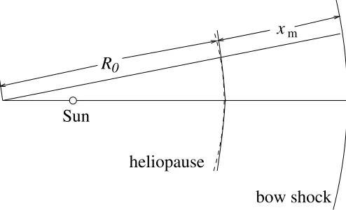
Fig. A.1.The sketch of spherical coordinate system. The heliopause and bow shock are shown by the solid lines. The spherical surface approximating the heliopause in the vicinity of the symmetry axis is shown by the dashed line.

Appendix A:

In this appendix we study the propagation of perturbations caused by the solar cycle variation in the outer heliosheath. We restrict our analysis to the vicinity of the symmetry axis. In this vicinity the heliopause can be approximated by a spher-ical surface with the radiusR0equal to the curvature radius of the heliopause at the symmetry axis, and with center on the symmetry axis at a distanceR0from the heliopause in the solar direction. We introduce spherical coordinates with center at the center of spherical surface and the radial coordinateR=R0+x (see Fig. A.1). In what follows we neglect the dependence of the background quantities on the angle coordinates and assume that they are functions of xonly. In addition, we neglect the velocity components in the angular directions. Hence, in the unperturbed state,ρ=ρ0(x),u=u0(x) andp=p0(x), whereu is the velocity in the radial direction, and the two other compo-nents of the velocity are zero.

We also assume that the wave motion is in the radial di-rection and depends onxonly. Then the wave motion is gov-erned by the system of gasdynamic equations with the right-hand sides describing the interaction between the plasma and the neutral gas.

We consider the heliopause oscillation as an external driv-ing force and put the boundary condition

u=ǫuˆsin (ωt) (A.1)

at the heliopause (x=0). Here ˆuis a characteristic speed near the heliopause andǫis a dimensionless parameter,ǫ_≪1.

An important quantity for our analysis is the sound speed

cS =(γp0/ρ0)1/2. In what follows we take ˆu=cS(0).

Let us now derive an approximate equation governing the propagation of nonlinear waves driven by the heliopause os-cillation in the outer heliosheath. The typical sound speed in the outer heliosheath is 20 km s−1_{. The wave period is} 11 years≈ 3.5×108 _{s. This gives the typical wavelength of} about 7×109 _km

≈50 AU. Since the outer heliosheath size along the symmetry axis is about 150 AU, we conclude that the characteristic wavelength is smaller that the characteristic

scale of inhomogeneity. This observation enables us to use the WKB approximation.

The propagation of nonlinear sound waves in homogeneous as well as in inhomogeneous media has been extensively stud-ied in nonlinear acoustics (e.g. Rudenko & Soluyan 1977) and in applications to the solar atmosphere (see, e.g., Narain & Ulmschneider 1990, and references therein). In particular, the equation governing the wave propagation has been de-rived under various assumptions about background quantities. However, for the reader’s convenience, we will briefly outline the derivation of the governing equation in what follows.

Our aim is to derive an equation that describes the com-bined effect of the nonlinearity and inhomogeneity. In accor-dance with this we assume that the small parameter charac-terizing the effect of inhomogeneity is of the same order as the small parameter characterizing the effect of nonlinearity, which isǫ. In other words, we assume that the ratio of the characteristic scales of perturbation and inhomogeneity isǫ. To show this explicitly we introduce the stretching variable σ = ǫxand assume thatρ0,u0 and p0 are functions of σ. In line with the WKB method we also introduce the running

vari-ableτ = t₋ǫ−1_{ϕ(σ), whereϕ(σ) is the eiconal. In the new}

variables we rewrite the system of governing equations as

∂ρ

∂τ−

dϕ dσ

∂(uρ)

∂τ +

ǫ ζ2

∂(uρζ2₎

∂σ =q1, (A.2)

∂u

∂τ−u

dϕ dσ

∂u

∂τ+ǫu ∂u

∂σ−

1 ρ

dϕ dσ

∂p

∂τ+

ǫ ρ

∂p

∂σ =q4, (A.3)

∂ ∂τ

p

ργ

−udϕ

dσ ∂ ∂τ

p

ργ

+ǫu ∂

∂σ

p

ργ

=q5, (A.4)

whereζ = ǫR =ǫR0+σ, andq4 andq5 can be expressed in terms ofq1,q2andq3. Recall that the right-hand sides of these equations describe the interaction between the plasma and the neutral gas. In what follows we neglect the effect of the neutral gas on the perturbations and assume thatq1,q4andq5do not change when the perturbations are introduced. We are looking for the solution to the system of Eqs. (A.2)–(A.4) in the form of expansions in power series with respect toǫ,

f = f0+ǫf1+ǫ2f2+. . . , (A.5)

wheref represents any of the quantitiesρ,uandp.

In the zero order approximation we collect terms of order unity in Eqs. (A.2)–(A.4). As a result we obtain the equations for the background quantitiesρ0,u0 and p0. The solution of these equations is shown in Fig. A.2, where the background density, ρ0, velocity, u0, and temperature, T0, are shown as functions of x. The background pressure p0 is calculated us-ing the relationp0=(2kB/mp)ρ0T0, wherekBis the Boltzmann constant andmpthe proton mass.

Fig. A.2.The dependences of background quantities in the outer he-liosheath on the distancexfrom the heliopause at the symmetry axis. The upper, middle and lower panels correspond to the density, veloc-ity and temperature. The densveloc-ity is given inρp,∞, the velocity invp,∞,

and the temperature in 104_{K. The distance xfrom the heliopause is} given in AU.

has a non-trivial solution only if its determinant is zero. This condition results in the equation determining the eiconal

1−u0 dϕ dσ

2

=c2_S

dϕ dσ

2

· (A.6)

In what follows we only consider waves propagating in the pos-itivex-direction. Then it follows from Eq. (A.6) that the eiconal is given by

dϕ

dσ =

1

cS +u0·

(A.7)

In addition, it follows thatρ1andp1can be expressed in terms ofu1as

ρ1= ρ0

cS

u1, p1=ρ0cSu1. (A.8)

In the second order approximation we collect terms of orderǫ2 in Eqs. (A.2)–(A.4). This results in the system of equations that,

with the aid of Eqs. (A.7) and (A.8), can be written as

cS

∂ρ2

∂τ −ρ0

∂u2

∂τ =

2ρ0

cS u1

∂u1 ∂τ

− cS_ζ+2u0 ∂ ∂σ

ρ0ζ2(cS +u0)

cS

u1

, (A.9)

cS

∂u2

∂τ −

1 ρ0

∂p2

∂τ =−(cS +u0) 2∂u1

∂σ

+(cS+u0)

1 ρ0cS

∂p0

∂σ −

1 ρ0

∂(ρ0cS)

∂σ −

∂u0 ∂σ

u1, (A.10)

∂p2

∂τ −c

2

S

∂ρ2

∂τ =(γ−1)ρ0u1 ∂u1

∂τ

−u1(cS +u0) ργ₀

cS ∂ ∂σ       p0 ργ₀

    

· (A.11)

This is a linear system of inhomogeneous algebraic equations with respect to∂ρ2/∂τ,∂u2/∂τand∂p2/∂τ. The determinant of this system is zero. This means that it has a non-trivial solution only if its right-hand side satisfies the compatibility condition. To obtain this condition we eliminate all the variables of the second order approximation from Eqs. (A.9)–(A.11). As a re-sult we arrive at

∂u1 ∂σ −λu1

∂u1

∂τ +µu1 =0, (A.12)

where the coefficient functionsλ(σ) andµ(σ) are given by

λ= γ+1

2(cS+u0)2

, (A.13)

µ= cS

2ρ0ζ2(cS +u0)2 ∂ ∂σ

ρ0ζ2(cS +u0)2

cS

· (A.14)

When the nonlinear term in Eq. (A.12) is neglected, it reduces to the equation of conservation of the wave action flux in a ra-dially expanding tube with the cross-section proportional toζ2, which isρ0ζ2(cS +u0)2u2₁/cS =const.

Let us return to the original independent variables, use the approximationu′_{≡u−u0≈ǫu1, and make the variable}

substi-tution

u′=U s(0)/s(x), (A.15)

where

u′=U s(0)/s(x), s=Rρ₀1/2c−_S1/2(cS +u0). (A.16)

Then Eq. (A.12) transforms to

∂U

∂x +

1

cS +u0

∂U

∂t −ΛU

∂U

∂t =0, (A.17)

whereΛ =λs(0)/s(x). In order to solve Eq. (A.17) we consider

xandUas independent variables, andtas a dependent variable, i.e.t=t(x,U). Then Eq. (A.17) transforms to

∂t

∂x =

1

cS +u0 −

V. Izmodenov et al.: Solar cycle e ects on the heliospheric interface,Online Material p 4

Integrating this equation we obtain

t=ϕ(x)−Uψ(x)+F(U), (A.19)

where

ϕ(x)=

x

0

d ˜x cS( ˜x)+u0( ˜x)

, ψ(x)=

x

0

Λ( ˜x) d ˜x, (A.20)

and the functionF(U) is determined by the boundary condi-tion (A.1). The right-hand side of Eq. (A.1) is a non-monotonic function oft. This implies that F(U) is a multi-valued func-tion. The periodic driving described by Eq. (A.1) causes peri-odic motion in the regionx>0. This observation enables us to consider only one wave period corresponding to−π_≤ωt_≤π atx=0. ThenF(U) is given by

F(U)=

                          

1 ω

−π₋arcsinU ǫuˆ

,₋π_≤ωt_{≤ −}π

2, 1

ωarcsin

U

ǫuˆ, −

π 2 ≤ωt≤

π 2, 1

ω

π₋arcsinU ǫuˆ

, π

2 ≤ωt≤π.

(A.21)

The inequalities forωthave to be satisfied atx=0.

Equation (A.19) determinesUas an implicit function oft

and x. In Fig. A.3 the evolution of the wave shape with the distancexfrom the heliopause is shown. The quantityUis dis-played as a function ofτ =t₋ϕ(x) for three different values ofx. The upper panel corresponds to x= 0, andU is a sinu-soidal function ofτ = t. When xincreases, the profile starts to steepen due to the action of nonlinearity. Eventually, this steepening results in a gradient catastrophe, which is the ap-pearance of infinite gradient at one particular point of the wave profile as shown in the middle panel of Fig. A.3. In order to determine the spatial positionxcand the point of the wave pro-file where the gradient catastrophe occurs, we note that at this point∂τ/∂U=∂2_τ/∂U2_{=0. Using Eqs. (A.19) and (A.21) we} rewrite these conditions as

ωˆuψ(xc)=

ǫ2₋U2−1/2, ωUǫ2₋U2−3/2=0. (A.22) It follows from these equations that the gradient catastrophe occurs at the point of the wave profile whereU=0, and at the spatial positionxcdetermined by the equation

ψ(xc)= 1

ǫωuˆ· (A.23)

If we formally use Eq. (A.19) for x > xc, then we obtainU as a multi-valued function ofτas shown in the lower panel of Fig. A.3. Such a multi-valued solution does not make physical sense. To obtain a physically meaningful solution we have to allow a discontinuity at a particular position of the wave pro-file. This discontinuity corresponds to a shock. It follows from the Rankine-Hugoniot relations at shocks that the velocity per-turbation at the two sides of the shock have the same magnitude and opposite signs (see, e.g., Rudenko & Soluyan 1977). It im-mediately follows from this condition and Eq. (A.19) that the shock position in the wave profile isτ= 0, and the shock in-tensityUsis determined by the equation and inequality

Us=ǫuˆsin (ωUsψ), 0< ωUsψ≤π/2. (A.24)

Fig. A.3.Evolution of the shape of the wave profile with the distance from the heliopause.U/ǫuˆis shown as a function ofωτ=ω[t−ϕ(x)]. The upper, middle and lower panes correspond to x= 0,x = xc ≈ 44.5 AU, andx= 70 AU. In the lower panel the dashed line shows the unphysical branch of the multivalues functionU(τ) determined by Eq. (A.19). The vertical solid line is the shock.

We have used Eqs. (A.23) and (A.24) to calculatexcand the de-pendence of the velocity jump at the shock,∆u=2Uss(0)/s(x). Using the numerically obtained value for the amplitude of the heliopause oscillation, 2 AU, and the fact that the oscillation period is equal to the solar cycle period, we immediately ob-tain thatǫuˆ _≈ 5.4 km s−1_{. Since ˆu = c}

S(0) ≈ 40 km s−1, we obtainǫ _≈ 0.135, so that the use of ǫ as a small parameter is justified. Usingǫuˆ _≈5.4 km s−1 _{and numerically calculated} functionsρ0(x),u0(x) andcS(x), we found that xc≈44.5 AU. Since the distance between the heliopause and the bow shock is about 140 AU, we conclude that the gradient catastrophe oc-curs inside the outer heliosheath.

In Fig. A.4 the dependence of ∆u on x is shown for

xc≤x≤xm, where xm ≈ 140 AU is the distance between the

Fig. A.4.The dependence of the velocity jump at the shock on the distancexfrom the heliopause. The velocity is given in km s−1_{, and} the distancexin AU.

Fig. A.5.The snapshots of the wave profile atωt=nπ,ωt=(n+1/2)π

andωt=(n+1)π, wherenis any integer number. The dotted vertical lines indicate the bow shock position. The velocity is given in km s−1 and the distance in AU.

dissipation at the shock reduces the wave energy flux by one and a half orders of magnitude in comparison with the value given by the linear theory.

Let us now consider the plasma heating due to the wave energy dissipation. The standard approach to solving this prob-lem is as follows. There are different timescales in the system. The first one is the wave period. The second is the characteris-tic time of variation of the background quantities caused by the additional momentum input due to the wave pressure and the energy input due to wave dissipation. To take the two different timescales into account we introduce two different times, “fast” and “slow”. Then we average governing equations with respect to the fast time. As a result we obtain the system of equa-tions describing the slow evolution of the background quan-tities. This system is very complicated and can be solved only

numerically. So, instead of using this approach, we will give only an estimate of plasma heating rate.

Let us consider the domain between the heliopause and the bow shock in the form of the frustum of a cone with the smaller base of radiusǫR0, larger base of radius ǫ(R0 +x+m), and heightxm, whereǫ≪1. Now we estimate the rate of the energy

increase in this domain due to wave damping. Up to now we have used the ideal description of the plasma motion. However, to calculate the rate of wave energy dissipation we need to take some dissipation mechanism/mechanisms into account. Since the dissipative coefficients are small, dissipation occurs only in thin layers that reduce to shocks in the limit of the ideal descrip-tion. As a result the rate of wave energy dissipation does not depend on what particular dissipation mechanism/mechanisms we take into account. Having this in mind we choose viscosity. The rate of energy dissipation per unit volume due to viscosity is given by

Hv=

4ρν 3

∂u′

∂x 2

, (A.25)

whereνis the kinematic viscosity. For waves with small am-plitude we can substituteρ0forρin this expression. Since vis-cosity is very weak, it is only important in the region of large gradients, i.e. in the vicinity of the shock position in the ideal description. This observation enables us to use the approximate description of the wave profile (see, e.g., Rudenko & Soluyan 1977). For x < xc we use the ideal description. For x > xc we use the ideal description for all moments of time except a small time interval embracing the moment of time when the shock passes this particular spatial position. This interval is de-termined by the inequality|ωτ_| δ=νω/ˆu2 _≪1 (recall that τ=t₋ϕ(x)). The solution of viscous hydrodynamic equations inside this interval describes the structure of the shock. It is given by (e.g., Rudenko & Soluyan 1977)

u′=u′_v≡ ∆u

2 tanh κ(x)ωτ

δ , (A.26)

whereκ(x) = (γ+1)cS∆u/4 ˆu2. Using the relation∂u′v/∂x ≈

(1/cS)∂u′v/∂τand Eq. (A.26), and taking into account that

dis-sipation occurs only in the thin layer_|ωτ_| δ, we obtain that the rate of energy dissipation per unit volume at the position

x>x0averaged over the wave period is

Hv ≈

4ρ0ν 3c2

S(2π/ω) δ/ω

−δ/ω _∂u′

v

∂τ

2

dτ (A.27)

≈ (γ+1)ωρ0(∆u)

3 24πcS

∞

−∞

dξ cosh4ξ =

(γ+1)ωρ0(∆u)3

18πcS ·

When deriving this expression we have used the fact that 1/coshξ decreases very fast when |ξ_{| → ∞} and substituted the lower and upper limits of integration by−∞and∞ respec-tively. To obtaine the rate of energy dissipation in volumeV

averaged over the period,Lv, we have to integrateHvoverV.

Taking into account thatHv = 0 forx < xc and using the numerical results, we obtain

Lv=πǫ2 xm

xc

Hv(R0+x)2dx≈2.8×1038ǫ2ωρp,∞v2p,∞ J/s,

V. Izmodenov et al.: Solar cycle e ects on the heliospheric interface,Online Material p 6

whereω,ρp,∞andvp,∞has to be measured in the SI units, i.e.

in s−1, kg/m3and m/s respectively. The total mass of the plasma in the considered domain is M _≈ 1041πǫ2ρp,∞ kg. We take cvM as an estimate for the thermal capacity of the plasma in

the domain, wherecvis specific heat at constant density. Since cv=2kB[(γ−1)mp]−1≈2.5×104 J K−1kg−1, we obtaincvM≈

2.5×1045_πǫ2_ρ

p,∞ J/K. Then, if we neglect all energy losses

from the domain, then its mean temperature will increase by

(2π/ω)Lv/cvM≈2.2×10−7v2p,∞K≈150 K. (A.29)