233
DEVELOPMENT OF ARTIFICIAL NEURAL NETWORK MODEL IN PREDICTING PERFORMANCE OF THE SMART WIND TURBINE BLADE
Supeni E.E.1, Epaarachchi J.A.2, Islam M.M.2 and Lau K.T.2,3
1
Dept. of Mechanical Eng., Faculty of Engineering, Universiti Putra Malaysia, Malaysia 2
Centre Excellence Engineered in Fibre Composites, University of Southern Queensland, Australia 3
Dept. of Mechanical Eng., Hong Kong Polytechnic University, Hong Kong [email protected]
ABSTRACT
This paper demonstrates the applicability of Artificial Neural Networks (ANNs) that use Multiple Back-Propagation networks (MBP) and Non-linear Autoregressive with Exogenous (NARX) for predicting the deflection of the smart wind turbine blade specimen. A neural network model has been developed to perform the deflection with respect to a number of wires required as the output parameter. The parameter includes load, current, time taken and deflection as input parameters. The network has been trained with experimental data obtained from experimental work. The various stages involved in the development of genetic algorithm based neural network model are addressed at length in this paper.
Keywords: Artificial neural network; back-propagation; multiple back-propagation;
non-linear autoregressive with exogenous.
INTRODUCTION
234
Figure 1. Bending moment against radius in a large turbine blade (Nolet 2011).
RESEARCHSIGNIFICANCE
The effect of current applied of SMA wires and correlation of the deflection of the plate has been modelled in ABAQUS in Figure 2 and tested experimentally in Figure 3 (ABAQUS 2012). The results obtained from the investigation were used to generate an ANN based design tool for predicting the amount of wire needed to restore the original shape of such bending. This depends on parameters such as deflection, the total current and the applied load.
235
Figure 3.Photograph of tested composite plate.
METHODOLOGY
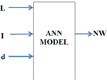
This study is to evaluate the predictive ability using Machine Learning (ML) which is MBP and NARX. The performance comparison between Multiple Back-Propagation (MBP) and Non-linear Autoregressive with Exogenous (NARX) are undertaken. To facilitate the performance comparison, all networks simulated have been designed and trained accordingly from output layers, hidden layers and output layers. Output neurons use hyperbolic tangent activation functions. The standard back-propagation algorithm is used to train the networks with learning rate equal to 0.01. Once a given network has been trained, it is required to provide estimates of the future sample values of a given time series for a certain prediction. The predictions are executed in a recursive curve until desired prediction horizon is reached, i.e., during Ntime steps the predicted values are fed back in order to take part in the composition of the regressors. The networks are evaluated in terms of the root mean square error (RMSE). The parameter such as applied load (L), applied current (I) and deflection (d) have been used as input and number of wire (NW) as the output to designed ANN. The general schematic diagram is illustrated in Figure 4.
Figure 4. General structure of model ANN.
[image:3.595.211.386.543.675.2]236
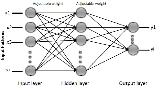
[image:4.595.171.424.183.325.2]MBP Method
Figure 5. Diagram of MBP network.
Figure 5 illustrates a learning process of multi-layer neural network employing back propagation algorithm. To illustrate this process the three layers neural network, for example, three inputs, three hidden layers and one output were implemented. Two types of sigmoid activation functions were selected for several numbers of hidden, output layer 2 which are logarithmic sigmoid function (logsig) and hyperbolic tangent sigmoid function (tansig) respectively. The adjustable weights used to propagate errors back were equal to the one used during computing output value. Only the direction of data flow was changed (signals are propagated from output to inputs one after the other). This technique was used for all network layers. For comparative study, a free opened source software has been used to generate the MBP which use program code C (Noel & Bernardete 2001; Noel & Bernardete 2003) .
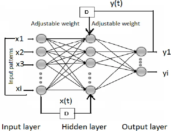
NARX Method
237
Figure 6. Diagram of NARX network.
RESULTSANDDISCUSSION
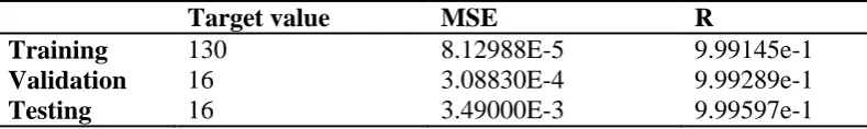
The number of SMA wires applied has been considered as an output vector. Applied current, deflection and load are considered as the input vectors. All calculations of neural network were made using MATLAB (Levenberg-Marquardt) and MBP open source code. The schematic diagrams of the both models are displayed in Figure 7 and 8. Both LM and MBP algorithms for training were applied to the network. The application randomly divides input vectors and target vectors into three sets, as follows. 80% are used for training. 10% are used to validate that the network is generalising and to stop training before over-fitting. The last 10% are used as a completely independent test of network generalisation. Data from experiments were collected to train the performance deflection number of wire with response to the load applied, deflection and the current applied. About 162 values of data were used for these networks. Table 1 shows NARX1 model with the lowest MSE among other model of ANNs and the fastest mode convergence training network. As can be seen from Table 2, the smallest values of MSE and the high values of R give us reason to consider the obtained NARX models as adequate which are almost to unity.
[image:5.595.141.457.627.714.2]238
[image:6.595.86.511.333.447.2]Figure 8. Example of MBP diagram network with 50-40 hidden layers.
Table 1.Predicting the deflection with respect to number of wires using various model.
Model Input
vector
Output vector
Structure/No hidden layer
neuron
Epoch (No. of Iteration)
Mean Square Error (MSE)
MBP1 L,I,d NW 50-40 1,273,277 0.009999 MBP2 L,I,d NW 50-40-30-20 437,788 0.009997 NARX1 L,I,d NW 10 delay time 2 26 0.000308 NARX2 L,I,d NW 10 delay time 3 10 0.001542 NARX3 L,I,d NW 10 delay time 4 7 0.002337
Table 2. The detail results of the NARX model training for NARX.
Target value MSE R
Training 130 8.12988E-5 9.99145e-1
Validation 16 3.08830E-4 9.99289e-1
Testing 16 3.49000E-3 9.99597e-1
[image:6.595.101.496.488.547.2]239
Figure 9. The network’s performance.
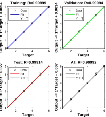
Figure 10. Regression analysis plot for the NARX .
2 4 6
1 2 3 4 5 6 Target O u tp u t ~ = 1 *T a rg e t + 0 .0 0 5
4 Training: R=0.99999
Data Fit Y = T
2 4 6
1 2 3 4 5 6 Target O u tp u t ~ = 1 *T a rg e t + 0 .0 0 3
4 Validation: R=0.99994
Data Fit Y = T
2 4 6
1 2 3 4 5 6 Target O u tp u t ~ = 1 *T a rg e t + 0 .0 2
7 Test: R=0.99914
Data Fit Y = T
2 4 6
1 2 3 4 5 6 Target O u tp u t ~ = 1 *T a rg e t + 0 .0 0
7 All: R=0.99992
[image:7.595.125.466.350.727.2]240
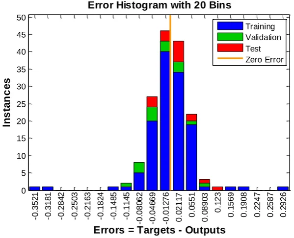
Figure 11. Error histogram of the NARX prediction model
Figure 12. Auto-correlation of errors of NARX prediction model and correlation between input and output with respect to target function.
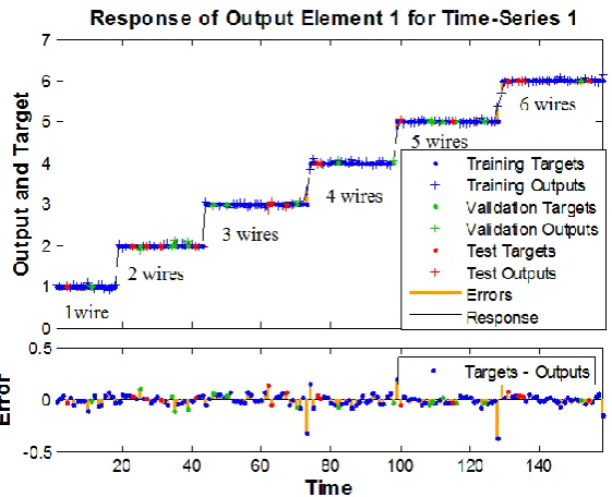
The correlation between input and error is provided in Figure 12. This figure illustrates how the errors are correlated with the input sequence. The perfect prediction model means that all the correlations should be zero. In this case, all of the correlations are within the confidence bounds around zero. The function of auto-correlations of errors is used to validate the network performance. Auto-correlation describes how the prediction errors are related in time. For the perfect model, there should be only one non-zero value of the auto-correlation at zero lag. This means that there is no correlation in prediction errors with each other. In this case, the correlations, except the one at zero lag, are within the 95% confidence limits. Based on the various diagnostics described up to now, it can be concluded that the model is adequate. Figure 13 confirms that the responses, obtained from the NARX prediction model for the performance deflection,
0 5 10 15 20 25 30 35 40 In s ta n c e s
Errors = Targets - Outputs
-0 .3 5 2 1 -0 .3 1 8 1 -0 .2 8 4 2 -0 .2 5 0 3 -0 .2 1 6 3 -0 .1 8 2 4 -0 .1 4 8 5 -0 .1 1 4 5 -0 .0 8 0 6 2 -0 .0 4 6 6 9 -0 .0 1 2 7 6 0 .0 2 1 1 7 0 .0 5 5 1 0 .0 8 9 0 3 0 .1 2 3 0 .1 5 6 9 0 .1 9 0 8 0 .2 2 4 7 0 .2 5 8 7 0 .2 9 2 6 Test Zero Error
-20 -15 -10 -5 0 5 10 15 20
-1 0 1 2 3 4
x 10-3 Autocorrelation of Error 1
[image:8.595.104.485.385.558.2]241
[image:9.595.154.435.174.402.2]are adequate, since the errors are quite small. For comparison, similar shape also has been obtained as shown in Figure 14. The predictions obtained based on both methods of network training, the NARX has improved the training network compared to the MBP networks. In MBP, there are still network output errors with respect to desired output network. Although the errors are not correlated with the input sequence, all the correlations are not within the 95% confidence limit.
Figure 13.Response of NARX prediction model for performance deflection (trained by the Levenberg- Marquardt algorithm)
Figure 14. The desired output and network output by MBP by opened source C code
CONCLUDINGREMARKS
[image:9.595.150.441.458.638.2]242
models are mainly dependent on the applied architecture and training method. Within the context of architecture, the behaviour of NARX models mostly depends on the numbers of neurons in hidden layers. Too many hidden neurons in network cause over-fitting that, in turn, leads to poor predictions. Future modeling of the NARX is to model ANN 2 and ANN 3 which use deflection and applied current as the output vectors respectively.
ACKNOWLEDGEMENT
The authors would like to thank the UPM and MOHE of Malaysia for providing the research facilities and support in CEEFC of University of Southern Queensland, Australia.
REFERENCES
ABAQUS 2012, ABAQUS/CAE Release Note 6.12
Composite Wind Blade Engineering and Manufacturing 2011
Gayan, CK 2012, 'Monitoring Damage in Advanced Composite Structures Using Embedded Fibre Optic Sensors', University of Southern Queensland Australia, Toowoomba
Gayan, CK, Jayantha, AE, Hao, W and Lau, KT 2013, 'Prediction of Obsolete FBG sensor using ANN for Efficient and Robust Operation of SHM Systems', Key Engineering Materials, no. 558, pp. 546-53.
Howard, D and Mark, B 2000, Neural Network Toolbox for Computation, Visualization and Programming-User's Guide
Noel, L and Bernardete, R 2001, 'Hybrid learning multi neural architecture', IEEE International Joint Conference on Neural Networks, vol. 4, pp. 2788-93.
Noel, L and Bernardete, R 2003, 'An Efficient Gradient-Based Learning Algorithm Applied to Neural Networks with Selective Actuation Neurons', Neural Parallel and Scientific Computations, vol. 11, pp. 253-72.
Peter, JS and Richard, JC 2012, 'Wind Turbine Blade Design, Review', Energies, vol. 5, pp. 3425-49
Sapuan, SM and Iqbal, MM 2010, Composite Materials Technology, Neural Network Applications, CRC Press Taylor and Francis Group
Sorensen, BF, Jørgensen, E, Christian, PD and Jensen, FM 2004, Improved Design of Large Wind Turbine Blade of Fibre Composites Based on Studies of Scale Effects (Phase 1)
Supeni, EE, Epaarachchi, JA, Islam, MM and Lau, KT 2012a, 'Design and Analysis of a Smart Composite Beam for Small Wind Turbine Blade Construction', Southern Region Engineering Conference (SREC), Australia Engineers, Queensland, USQ, Toowoomba, Australia