Faculty of Health, Engineering & Sciences
Model and Analysis of a Broken Conductor (Source
Isolated) Earth Fault on Radial 11kV Distribution
Feeders.
A dissertation submitted by
A. Geary
in fulfilment of the requirements of
ENG4112 Research Project
towards the degree of
Bachelor of (Electrical Engineering, Power Systems)
Protection schemes of electricity distribution networks are designed to limit the damage
to the network in the event of a fault, and to provide some security and safety to the
network. This thesis examines the electrical characteristics of the Source Isolated Earth
(SIE) Fault.
The Source Isolated Earth Fault is a type of high impedance earth fault that can occur
on overhead electricity networks. SIE faults are caused by a broken overhead conductor
falling to ground on the load side of the span with the source end of the span isolated
from the ground.
A simplified model for calculation of the earth fault levels in SIE faults was developed
by circuit reduction of the fault schematic. The SIE fault was reduced to the equivalent
of a Phase to Phase to Ground fault.
Results obtained from the simplified model were compared to two peer reviewed models
for SIE fault calculations in order to validate the simplified method. The comparison
was undertaken in two stages, by first varying one factor at a time to determine the
most significant factors and then by carrying out designed experiments on the significant
factors and analysing the interactions between these factors.
The results of the one factor at a time analysis identified which of the factors had the
largest effect on the earth fault current. The most significant factor in determining
the earth fault level in SIE faults is the pre-fault load beyond the fault location. This
knowledge can be used to identify areas where SIE fault levels may be low.
Computational efficiency of the three models was compared using MATLAB profiling.
Confidence in the theory was bolstered by the calculation of fault levels for a case
study. The results were compared between all three models and data captured during
an actual SIE fault event.
A process was developed that allowed existing 11 kV network feeder models to be
analysed using the SIE fault models. Sections of feeder where SIE fault levels may be below conventional Sensitive Earth Fault (SEF) protection pickup levels were identified.
Attempts to optimise the feeder analysis led to methods of reducing the number of
network nodes to be tested to find the limit of the protection zone.
The extreme case analysis led to the discovery of the circuit conditions that must exist
for these types of faults to be undetectable by conventional SEF protection schemes.
It was discovered that the maximum possible SIE fault current can be easily estimated
Faculty of Health, Engineering & Sciences
ENG4111/2 Research Project
Limitations of Use
The Council of the University of Southern Queensland, its Faculty of Health,
Engineer-ing & Sciences, and the staff of the University of Southern Queensland, do not accept
any responsibility for the truth, accuracy or completeness of material contained within
or associated with this dissertation.
Persons using all or any part of this material do so at their own risk, and not at the
risk of the Council of the University of Southern Queensland, its Faculty of Health,
Engineering & Sciences or the staff of the University of Southern Queensland.
This dissertation reports an educational exercise and has no purpose or validity beyond
this exercise. The sole purpose of the course pair entitled “Research Project” is to
contribute to the overall education within the student’s chosen degree program. This
document, the associated hardware, software, drawings, and other material set out in
the associated appendices should not be used for any other purpose: if they are so used,
it is entirely at the risk of the user.
Dean
I certify that the ideas, designs and experimental work, results, analyses and conclusions
set out in this dissertation are entirely my own effort, except where otherwise indicated
and acknowledged.
I further certify that the work is original and has not been previously submitted for
assessment in any other course or institution, except where specifically stated.
A. Geary
Q9222672
Signature
This thesis was produced with guidance and assistance of my supervisor Dr Tony
Ah-fock. My thanks to him for the assistance provided.
My thanks to my employer Essential Energy for without their assistance I could not
have found the resources to embark on such a great mission as a BENG.
I also must acknowledge the persistence and patience of my wife Katrina and my sons
Nathan, David, Daniel and Stephen. Without their assistance in the matters that
would otherwise distract me from my studies, none of this would be possible.
A. Geary
Abstract i
Acknowledgments v
List of Figures x
List of Tables xiii
Chapter 1 Introduction 1
1.1 The Broken Conductor (Source Isolated) Earth Fault . . . 1
1.2 Overview of the Thesis . . . 3
1.3 Project Objectives . . . 4
Chapter 2 Literature Review 5 2.1 Literature Review . . . 5
2.2 Conventional Earth Fault and Sensitive Earth Fault Protection . . . 5
2.3 Non Conventional Protection . . . 7
2.4 Sequence Components Methods . . . 8
2.6 Blackburn Model . . . 12
2.7 Phase to Phase to Ground Fault Model . . . 12
2.8 Consequences of Undetected Faults . . . 13
2.9 Frequency of Source Isolated Earth Faults . . . 14
Chapter 3 Modelling Methodologies 15 3.1 Building MATLAB models . . . 15
3.1.1 Building the Burgess Model . . . 17
3.1.2 Building the Blackburn Model . . . 20
3.1.3 Deriving the Simplified (Phase to Phase to Ground Fault) Model 22 3.1.4 Line Capacitances Added to Models . . . 27
3.1.5 Single Phase Model . . . 29
3.2 Sensitivity Analysis . . . 33
3.2.1 OFAT Testing . . . 33
3.2.2 Designed Experiments . . . 44
3.2.3 Code Profiling . . . 46
Chapter 4 Case Study 48 4.1 Comparison of Results . . . 48
Chapter 5 Feeder Studies 51 5.1 Feeder Calculation Minimisation . . . 51
5.3 Extreme Case Analysis . . . 55
5.3.1 Three Phase Extreme Case Analysis . . . 55
5.3.2 Single Phase Extreme Case Analysis . . . 59
5.3.3 Summary of Extreme Case Analysis . . . 62
5.3.4 Effect of Increasing SEF Protection Sensitivity . . . 64
5.4 Mechanical Factors . . . 66
Chapter 6 Conclusions and Further Work 68 6.1 Achievement of Project Objectives . . . 68
6.2 Conclusions . . . 69
6.3 Recommendations . . . 70
References 71 Appendix A Project Specification 74 Appendix B MATLAB Code 76 B.1 TheFeederProcess.mMATLAB Script . . . 77
B.2 ThefuncBBL.m MATLAB Function . . . 80
B.3 ThefuncBBLWLC.m MATLAB Function . . . 83
B.4 ThefuncBurgess.mMATLAB Function . . . 86
B.5 ThefuncBurgessWLC.m MATLAB Function . . . 89
B.6 ThefuncGraphI.m MATLAB Function . . . 92
B.8 ThefuncIEFWLCAP.m MATLAB Function . . . 96
B.9 ThefuncParallelZ.mMATLAB Function . . . 100
B.10 ThefuncPPE.m MATLAB Function . . . 101
B.11 ThefuncPPEWLC.m MATLAB Function . . . 103
B.12 ThefuncPUPhase2Seq.m MATLAB Function . . . 105
B.13 ThefuncPUSeq2Phase.m MATLAB Function . . . 106
B.14 ThefuncSPE.m MATLAB Function . . . 107
B.15 TheIsolatedEarthFault.mMATLAB Script . . . 109
B.16 TheMultiVariableAnalysis.mMATLAB Script . . . 113
1.1 Pictorial representation of the fault condition. . . 2
2.1 General CT arrangement for feeder CTs. . . 6
2.2 Sequence components of unbalanced phase values. . . 9
3.1 Schematic diagram of Source Isolated Earth Fault. . . 16
3.2 Sequence connections diagram (from the code in Burgess(2011)). . . 18
3.3 Sequence connections diagram from Blackburn(1993). . . 20
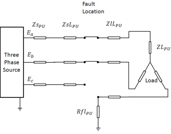
3.4 Schematic of three phase Source Isolated Earth Fault. . . 22
3.5 Fault schematic of Source Isolated Earth Fault with star equivalent load impedance. . . 23
3.6 Fault schematic reduced by series addition. . . 24
3.7 Fault schematic reduced to phase to phase to ground equivalent. . . 25
3.8 Sequence network connections diagram for phase to phase to ground faults. 26 3.9 Nominal Π circuit of a medium length transmission line. . . 27
3.10 Circuit simplification to include line capacitance. . . 28
3.12 Single phase Source Isolated Earth Fault schematic. . . 30
3.13 Fault schematic reduced to the equivalent of a phase to ground Fault. . 31
3.14 Sequence network connections diagram for phase to ground faults. . . . 32
3.15 OFAT results for pre-fault voltage. . . 34
3.16 OFAT results for source impedance . . . 35
3.17 OFAT results for upstream network impedance . . . 37
3.18 OFAT results for downstream network impedance . . . 38
3.19 OFAT results for upstream network capacitive reactance.. . . 39
3.20 OFAT results for downstream network capacitive reactance. . . 40
3.21 OFAT results for downstream load impedance. . . 41
3.22 OFAT results for fault impedance. . . 42
3.23 Source Isolated Earth Fault schematic. . . 44
3.24 Combined graph of 10 variations in upstream, downstream, load and fault impedances. . . 46
3.25 Matlab profiler results. . . 47
4.1 Google Earth view of the approximate fault location. . . 49
5.1 Sample CBD feeder with areas of low Source Isolated Earth Fault current highlighted in red. . . 53
5.2 Healthy three phase network schematic. . . 55
5.3 Extreme case healthy three phase network schematic. . . 56
5.5 Extreme Case Single Phase Load Schematic. . . 60
5.6 Extreme Case of Source Isolated Fault on single phase network. . . 61
5.7 Sample 11kV rural feeder with undetectable areas shaded in red (5A
SEF pickup). . . 64
5.8 Sample 11kV rural feeder with undetectable areas shaded in red (1A
3.1 Unknown quantities in Burgess model. . . 18
3.2 Summary of OFAT results. . . 43
4.1 Summary of case study results for various values ofRf l . . . 50
Introduction
In a three phase network designed for the distribution of power there are many types of
faults which may occur. The more common types of faults are the three phase fault, the
single phase to ground fault, the phase to phase fault, and the phase to phase to ground
fault. As well as these common types of faults there are some more obscure faults which
may occur only infrequently on the system. It was one of these less frequent anomalies that was the focus of this thesis.
1.1
The Broken Conductor (Source Isolated) Earth Fault
In an overhead 11kV distribution network the conductors are strung through the air by
being suspended on insulators at each pole. The poles can be of significant height and
have significant separation between them. It is possible that an overhead conductormay break. When a conductor breaks the two parts of the broken conductor fall towards
the ground. The conductor ends may or may not come into contact with the ground,
depending on the heights of the poles and the location of the break.
This thesis focuses on those instances where an overhead conductor breaks and the
source side of the broken conductor is suspended from the ground due to the position
of the break in the conductor span and the load side of the conductor makes electrical
contact with the ground.
Figure 1.1: Pictorial representation of the fault condition.
earth for fault current is down the healthy two phases, through the downstream load
and back along the faulted phase and to ground through the fault impedance. A
schematic diagram for this fault condition is shown in Figure 3.1.
The fault current may be very limited in these situations, depending on the system configuration and load. As such this type of fault may be difficult to detect. Work has been undertaken in this thesis to develop a simplified method of estimating the fault
current in these conditions. Some reports indicate that no accurate means of detecting
this type of fault exist.
The aim of the thesis is to gain an understanding of the electrical nature of the Source
Isolated Earth Fault by understanding the dominant factors that affect the fault
lev-els developed by this type of fault. Methods were developed to identify where these
faults may be undetectable by conventional earth fault and Sensitive Earth Fault (SEF)
protection schemes.
Peer reviewed methods were discovered during literature review and these were
com-pared to verify the derived method.
Calculations were compared to results taken from an actual case study. The case study
includes actual results from sophisticated metering installed on a feeder where one of
Sensitivity analysis was undertaken to ascertain the dominant factors which controlled
the level of earth fault current. This knowledge was then applied to feeder topography
to illustrate where this fault may be undetectable by conventional Sensitive Earth Fault
protection.
A means of identifying where SEF protection pickups are not possible was developed
by further analysis of the fault condition.
Further references to this type of fault in this document will refer to it as a source
isolated earth fault (SIEF).
1.2
Overview of the Thesis
This thesis is organized as follows:
Chapter 1 provides an introduction to the Source Isolated Earth Fault, and describes
an overview and scope of the thesis.
Chapter 2 describes the significant findings uncovered by the literature review and
discusses the modelling methods employed in analysing the Source Isolated Earth
Fault.
Chapter 3 discusses Matlab functions designed according to the peer reviewed models.
A new model for the solution of the Source Isolated Earth Fault is derived. Testing
of the models was carried out to find the significant factors that determine the
severity of this type of fault. The models were also compared to ensure that the
derived model is an adequate method for estimating the fault currents.
Chapter 4 compares the model results with an actual recorded case study. This
provided confidence in the models before expanding their application to testing
SEF pickup on entire feeders.
Chapter 5 applies the models to test SEF pickup on example feeders and analyses
the results, the analysis culminates in a derivation of an extreme case that can
be used to estimate the maximum level of earth current possible in the case of a
Chapter 6 concludes the dissertation and recommends further work in the area of
un-derstanding the mechanical factors that are required to allow the Source Isolated
Earth Fault to occur.
1.3
Project Objectives
The purpose and intent of the thesis is to;
• Model the broken conductor fault in an 11 kV overhead distribution feeder.
(broken conductor near the line side of span such that only the load side of the
broken conductor hits the earth, the line side is isolated).
• Investigate the circumstances where this fault is not detectable using ’traditional’
EF/SEF protection schemes.
These objectives are investigated by performing the following;
1. Research the background information relating to the Source Isolated Earth Faults
on 11kV radial distribution feeders.
2. Develop MATLAB code to model the behaviour of this particular type of fault.
3. Compare the models with calculations for calibration / accuracy check of the models.
4. Investigate the factors which influence the fault levels by carrying a sensitivity
anal-ysis on the models to find the dominant factors.
5. Apply the models to a case study of an actual fault on an 11kV feeder.
6. Investigate the likelihood of this type of fault occurring.
7. Derive conclusions and recommendations from any noteworthy discoveries.
The aims and objectives are stated in the project specification, which was developed
in conjunction with and approved by the project supervisor at the beginning of the
Literature Review
2.1
Literature Review
Following is a summary of the relevant discoveries made during the literature review
that assisted in the understanding of this project and provided some background
infor-mation that assisted in formulating the thesis.
During the literature review it was discovered that two recent works explored this
fault and provided methods for the calculation of fault currents developed in source
isolated earth fault conditions. The following sections of the report describe the relevant
discoveries of the literature review.
2.2
Conventional Earth Fault and Sensitive Earth Fault
Protection
Earth Fault (EF) and Sensitive Earth Fault (SEF) schemes are employed in earthed
transmission and distribution systems. One of the main purposes of applying a reference
to earth for a system is so that the system will be able to develop enough (earth fault)
current when an active conductor faults to earth to allow the protection to detect the
fault and operate circuit breakers to isolate the fault.
and protection functions. The protection equipment is isolated from the distribution
voltages by means of Current Transformers (CTs) and Voltage Transformers (VTs).
The CTs and VTs sample the high voltage distribution system currents and voltages
(respectively). The CTs have a transformation ratio. The CT transformation ratio is
the fixed ratio of current that the CT will provide as a sample to the protection circuits.
Distribution networks are based around a three phase system. This is a system of 3
separate conductors, which are electrically isolated from each other. As the mechanical
means of creating energy for a three phase electrical system involves alternators with
a rotating magnetic field inducing voltages on windings that are physically 1200 apart on the stators. The voltages that are created on the three phase output are electrically
1200 apart.
A common arrangement for the CTs is shown in Figure 2.1 (Horowitz & Phadke 2008).
On any particular feeder CTs will be installed on each phase. The CTs will produce
Figure 2.1: General CT arrangement for feeder CTs.
current in their secondaries to maintain the ampere-turn balance. 11kV distribution
feeder CTs commonly have transformation ratios of 500:1. This means that 500 A
in the primary (high voltage) circuit will be transformed into 1 A in the secondary
protection circuits. The transformation is a linear response, so that protection settings
can be achieved by applying the ratio directly (within specified limits of error).
protection. The relay labelled 4 in this figure would be the position in the circuit for
an EF/SEF relay. In this configuration the EF/SEF relay receives the sum of the three
phase currents, providing it with a representation any earth fault current.
The SEF relay is set to lower values of pickup, than an EF relay. The pickup setting of
a relay is the current that the relay will operate at. The pickup value referred to here
will be in terms of the primary current. For the purposes of this thesis it was assumed
that a 5A SEF pickup setting was the equivalent of 5 Amperes of primary current. As
the SEF protection has the most sensitive (lowest) setting, it will be considered as the
lower limit of when an earth fault will be detected by conventional protection schemes.
2.3
Non Conventional Protection
Non-conventional protection is outside the scope of this thesis. It is briefly mentioned
here to highlight the fact that ongoing research us taking place in this field.
Literature was found describing alternative means for detecting high impedance faults
(other than conventional EF/SEF protection schemes) (Al-Dabbagh, Daoud & Coulter
1989, Benner & Russell 1997, Sarlak & Shahrtash 2008, Sarlak & Shahrtash 2011,
Tor-res G & Ruiz P 2011), however literature was also found that explained that the
alternative methods where not suitably accurate due to a lack of discrimination,
selec-tivity, or reliability (Li & Redfern 2001, Lukowicz, Michalik, Rebizant, Wiszniewski &
Klimek 2010).
The alternate methods appear to be unreliable as they would not pick-up on known
faults and they would also false-trigger sometimes. Tengdin, Baker, Burke, Russell,
Jones, Wiedman & Johnson (1996) discussed various types of high impedance
protec-tion and found that they were approximately 80% effective.
Depew, Parsick, Dempsey, Benner, Russell & Adamiak (2006) carried out tests of
detecting known faults by post processing the captured data and found that only 58%
of downed conductors could have been detected.
Little information was given on the distances or the exact nature of the detected faults
level of earth fault current in the specific case of a source isolated earth fault on 11kV
distribution networks.
2.4
Sequence Components Methods
Methods have been developed to analyse networks to calculate the prospective fault
cur-rents for complicated fault situations (Mortlock 1947, Blackburn 1993, Burgess 2011).
These methods build on the efforts of Fortescue (1918).
Some background information is necessary before embarking on explanations of these
methods.
A method has been developed by Fortescue (1918) to use symmetrical components
to assist in solving asymmetrical faults in symmetrical multi-phase systems. For the
three phase power networks these components are the positive, negative, and the zero
sequence components.
The sequence on a network can be determined by observing the order its phase values
(voltage or current) reach their respective peaks. For example, in the power system
there are three phases. The three phases are nominated A, B, and C. Any configuration
whereby the phase voltages reach their maximum value in the order A, B, and then
C, would be considered a positive phase sequence. Due to the cyclical nature of three
phase networks a positive sequence network can equally be represented by CAB, or
BCA as only the starting point changed, not the sequence. In a negative sequence the
order of the phases would be reversed, ie ACB, BAC, or CBA depending on the starting
point for observing the sequence. In a zero sequence the phases peak at the same time
and are said to be in phase, as there is zero phase angle displacement between them.
As mentioned in section 2.2 the phase components in a three phase network are
sepa-rated by an angle of 120 degrees. As the phase values have a magnitude and an angle,
the phase values can be diagrammatically represented as vectors in a complex plane.
For the purposes of this thesis the conventional anticlockwise rotation will be assumed
for the determination of the sequence of phase values.
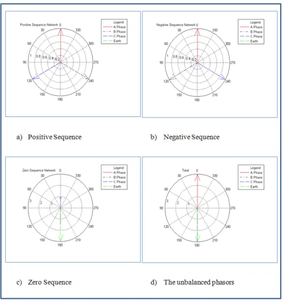
appear as shown in the vector diagrams shown in Figure 2.2.
Figure 2.2: Sequence components of unbalanced phase values.
In the case of the positive sequence values, shown in Figure 2.2 a) the phase values will
present in the order A, B, C as they rotate anticlockwise. The negative sequence values
in Figure 2.2 b) will present in the order A, C, B. The zero sequence values appear all
together in parallel as shown in Figure 2.2 c). Each of the sequences is a balanced set
of three vectors (representing 3 voltages or currents). This balance refers to each vector
in a sequence as having the same magnitude, the angle between phases is determined
by the sequence.
Each vector within these sets is known as a phasor. Each sequence may be represented
as one phase value only in calculations as the phase relationships to the other phasors are
unbalanced situation shown in Figure 2.2 d) may be represented by three vectors, where
each vector is a representation of a sequence group of 3 vectors. For consistency when
sequences are represented in this way it is usual for each of the sequence components
be represented by a vector of the same phase.
The sequences can be identified by using either a superscript +, -, or 0, or the numbers
1, 2, or 0 to represent the positive, negative or zero sequence current values as follows;
I+ = I1(positive sequence current)
I− = I2(negative sequence current)
I0 = I0(zero sequence current)
Likewise the superscripts/subscripts for voltages V+ = V1, V− = V2, V0 = V0 and
impedance (Z+ = Z
1, Z− = Z2, Z0 = Z0) follow the same pattern for the positive,
negative and zero sequence values of these quantities.
For each network element, sequence impedances must be derived (Grainger & Stevenson
1994) or measured so that networks can be constructed for each of the sequences. For
example, a line may have its positive sequence impedance measured by applying a three
phase voltages to one end with the other ends shorted together, and measuring the
currents. The negative sequence impedance may be measured using the same method,
but swapping two phases. The zero sequence impedance would require all three lines
to have exactly the same phase on each line, with the remote ends earthed, to carry
out the test. In this way the sequence impedances reflect the behaviour of the network
element with only that sequence of currents flowing through it.
The sequence impedances are then connected in various ways depending on the fault
situation, so that the sequence currents can be calculated. Once the sequence currents
are known, then the phase currents may be calculated by summation of each of the
phase currents in each of the sequence groups. When sequence networks are connected
to calculate sequence currents only the positive sequence network has a voltage source,
and it is a positive sequence source. The voltage of the source is the pre-fault voltage
on the network.
A total of nine sequence currents are required to fully describe an unbalanced set of
known, only 1 of each sequence is calculated. This means that an unbalanced group of
three phase currents can be described by one current from each of the sequences.
Mathematically the values can be converted between phase currents and sequence
cur-rents by the use of a couple of transformation matrices as follows:
To understand the matrix transformations it is necessary to introduce thea operator.
The a operator is a mathematical representation of a rotation of 1200 in the complex number plane (Horowitz & Phadke 2008).
a = 16 1200 =−0.5 +i
√
3 2
a2 = 16 2400 =−0.5−i
√
3 2 a3 = 16 00 = 1
IfIa, Ib, Icare the A phase, B phase and C phase currents respectively, andI+, I−, andI0 are the positive, negative and zero sequence currents then;
I+ I− I0 =
1, a , a2 1, a2, a
1, 1, 1
× Ia Ib Ic (2.1)
The transformation provided in equation 2.1 allows phase currents to be transformed
into the sequence components. This transformation is provided in Matlab code funcPUPhase2Seq.m
in Appendix B, Section B.12.
An inverse transformation is also available.
Ia Ib Ic =
1 , 1, 1
a2, a , 1 a , a2, 1
× I+ I− I0 (2.2)
The transformation provided in equation 2.2 allows sequence currents to be
trans-formed into the phase currents. This transformation is provided in Matlab code
2.5
Burgess Model
Burgess (2011) describes a method for calculating the currents in a system where a
broken conductor exists and either (or both) sides of a failed span provide an electrical
circuit to ground.
Burgess (2011) included a neutral earthing impedance as this was the primary focus
of that thesis, this was however easily accounted for and a modified circuit was easily
derived by changing the impedance of this branch.
The Burgess model is rather complicated as it allows for the solution of a fault on either
side of the broken span. This complexity results in a method involving 18 simultaneous
equations to calculate the sequence currents that flow.
Burgess provided Matlab code for this method which could be used directly to solve
the system and offered a means of comparison of the other methods discussed here.
2.6
Blackburn Model
Blackburn (1993) provides a method for the calculation of the currents when the Source
Isolated Earth fault occurs. The mathematical method is simplified (in comparison the
Burgess method) as only the Source Isolated Earth Fault is considered by this method.
One issue with this method is that the effect of fault impedance is not included.
There-fore this method needs to be modified to include the effects of a fault impedance. It is
necessary to develop Matlab code to model this calculation method.
2.7
Phase to Phase to Ground Fault Model
This method was discovered by circuit analysis of the fault schematic and reducing the
circuit to provide a simplified circuit. The circuit simplification was ceased when the
circuit resembled a phase to phase to ground fault as a method existed (Horowitz &
Applying the standard arrangement of sequence components for a Phase to Phase to
Ground Fault provided a simplified method of understanding the fault conditions.
The motivation for developing this model of the fault was that the phase to phase
to ground fault appeared to be simplified compared to the Burgess and Blackburn
models that each included transformers in the sequence circuits to represent similar
current flows in different parts of the circuit. The phase to phase to ground model does
not contain such contrivances, and as such is easier to understand without additional
explanation.
No literature was found on the application of a phase to phase to ground method for the
calculation of ground currents present in the case of a Source Isolated Earth Fault. The
use of this method to solve the fault condition is considered one of the major research
findings of this thesis. The steps to deriving this model are shown in the following
chapter.
2.8
Consequences of Undetected Faults
In some circumstances a Source Isolated Earth Fault may result in an earth current
that is too small to detect and as such the faulted conductor may remain alive on
the ground (Curk & Koncnik 1999). Depew et al. (2006) reported that, in a two year
period, Potomac Electric power Company (Pepco) documented 71 cases where downed
conductors were not cleared by conventional protection (Depew et al. 2006).
Subsequent activity in the vicinity of the downed conductor by animals or humans could
be dangerous or fatal (Toader, Blaj & Haragus 2007). Public education campaigns are
run by electricity distributors to advise customers to stay away from fallen power lines
(Essential Energy 2013).
Customers downstream of the downed conductor will experience quality of supply issues
associated with the loss of one HV conductor. In the case of the Source Isolated Earth
Fault the downed conductor may be close to earth potential if the fault impedance is sufficiently low. The downed conductor could also be at a voltage well above earth
potential, up to a voltage approximately between the two healthy phase voltages. The
phases with significantly less than nominal voltage.
This situation is called a brown out. The low voltages may cause damage to some
equipment if the brown out situation continues for some time. In cases where the
protection fails to clear the fault customer initiated quality of supply complaints, or
customer initiated reports of a wire downmay bethe only alert received by the network provider of the abnormal condition.
2.9
Frequency of Source Isolated Earth Faults
Source Isolated Earth faults are an extremely rare occurrence. A review of outage
information provided by Essential Energy was undertaken to identify any HV conductor
faults which may have been this type of fault.
Essential Energy provides energy services to over 800,000 homes and businesses in
N.S.W. (Essential Energy 2013), through a network of over 200,000km of power lines.
Essential Energy maintains over 1.4 million poles and 135,000 distribution substations.
Essential Energy is responsible for electricity network covering approximately 95% of
the state of New South Wales.
Network outage data was provided for the five year period from June 2008 to July
2013 (Gillespie & Matheson 2013). The fault information covered over 120,000 faults.
Overhead conductors were reported on the ground in 3453 of these faults. Apart from
the fault used for the case study in this thesis only two other faults werepossibly source isolated earth faults, where the fault information indicated that this type of fault may have occurred. These two incidences were found to involve 22kV circuits, which are
outside the scope of this thesis.
No reports of a Source Isolated Earth fault on 11kV circuits were found in the previous
five years of data provided by Essential Energy for use in this thesis. The analysis of
the outage data confirmed the rarity of this event.
Modelling Methodologies
3.1
Building MATLAB models
Matlab was the software chosen for the creation of code to solve the mathematical
calculations for the various models used in this thesis. Matlab is very versatile, powerful
mathematical software. The program flow functions available in Matlab made it easy
to deal with the matrix algebra required to solve some of the models.
To assist in the formulation of the function code for each of the modelling methods a
common set of input arguments was required. The sensitivity analysis tested each of
these system parameters in turn for a review of their significance. To facilitate this, the
Matlab functions were given an input variable for each electrical element of the network.
Most electrical elements required positive, negative and zero sequence components to
fully describe the behaviour of the network element in each of the sequence networks.
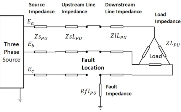
Figure 3.1 shows a schematic representation of the fault condition. This schematic is
the basic circuit for the fault and forms a common starting point for the models. The
terms in this diagram are;
ZsP U is the Source Impedance. The source was modelled as an infinite source feeding
through the source impedance. The source impedance was a Thevinin equivalent
Figure 3.1: Schematic diagram of Source Isolated Earth Fault.
ZsLP U is the PU impedances of the network, upstream of the fault location. ZsLP U contains the positive, negative and zero sequence impedances.
ZlLP U is the PU impedances of the network, downstream of the fault location. ZlLP U contains the positive, negative and zero sequence impedances. The downstream
network impedance used in the calculations was half of the actual network impedance.
This takes into account the fact that the downstream network loads are
dis-tributed along the feeder. Halving the impedance provides a means of estimating
the effects of distributed load by applying a lumped load at the end of half of the
actual network impedance (Vempati, Shoults, Chen & Schwobel 1987).
ZLP U is the PU impedances of the downstream load. The load impedance was
as-sumed to be balanced across the available phases.
Rf lP U is the label indicating the PU fault impedance.
ZcsP U and ZclP U represent the upstream (ZcsP U) and downstream (ZclP U) network
3.1.1 Building the Burgess Model
Burgess (2011) provided Matlab code for the solution of a broken conductor fault with
a fault impedance to ground on either side of the broken conductor. The application
in Burgess (2011) was related to the use of Arc Suppression Coils in the earthing
circuit as an aid to detecting various high impedance faults. This detection method
was interesting, and may show some promise, however it is outside the scope of this thesis. The provided method was adapted to the focus of this thesis very easily.
There were some inconsistencies noticed in the labelling of the original figure and the
subscripts used in the math equations, however the Matlab code was correct. The
inconsistencies were detected and corrected by going back to the work of Mortlock
(1947) and correcting some minor typographical errors in Burgess. These corrections
Figure 3.2: Sequence connections diagram (from the code in Burgess(2011)).
Table 3.1: Unknown quantities in Burgess model.
1 2 3 4 5 6 7 8 9 10 11 12 13 14 15 16 17 18
I1+ I1− I0 1 I
+ 2 I
−
2 I20 I + 3 I
−
3 I30 I + 4 I
−
4 I40 V +
S V
−
S V
0
S V
+
L V
−
L V
0
L
Figure 3.2 shows the connections of the sequence networks as defined in the code.
From Figure 3.2 it can be seen that there are 18 unknown symmetrical quantities in
this representation of the sequence network connections. The unknowns are shown in
The sequence currents are obtained by solving the system of 18 simultaneous equations
(Burgess 2011).
The equations are as follows;
VL+−I4+ZL+ = 0 (3.1)
VL−−I4−ZL− = 0 (3.2)
VL0−I40ZL0 = 0 (3.3)
VS+−I1+ZS+ = ES (3.4)
VS−−I1−ZS− = 0 (3.5)
VS0−I10ZL0 = 0 (3.6)
VS+−I4+ZL+−VS−+VL− = 0 (3.7)
VS−−I4−ZL−−VS0+VL0 = 0 (3.8)
I1+−I2+− V
+
S 3Rf S
− V
−
S 3Rf S
− V
0
S 3Rf S
= 0 (3.9)
I3+−I4+− V
+
L 3Rf L −
VL− 3Rf L −
VL0
3Rf L = 0 (3.10)
I20+I2−+I2+ = 0 (3.11)
I30+I3++I3− = 0 (3.12)
I1−−I2−− V
+
S 3Rf S
− V
−
S 3Rf S
− V
0
S 3Rf S
= 0 (3.13)
I10−I20− V
+
S 3Rf S −
VS− 3Rf S −
VS0
3Rf S = 0 (3.14)
I3−−I4−− V
+
L 3Rf L
− V
−
L 3Rf L
− V
0
L 3Rf L
= 0 (3.15)
−I40+I30− V
+
L 3Rf L
− V
−
L 3Rf L
− V
0
L 3Rf L
= 0 (3.16)
I2+−I3+ = 0 (3.17)
I2−−I3− = 0 (3.18)
The Matlab code from Burgess (2011) has been copied into a function in Matlab for
calculations to be efficiently made. The Matlab function funcBurgess.m is included in
3.1.2 Building the Blackburn Model
Blackburn (1993) presented a calculation method for Source Isolated Earth Fault
prob-lems. The method offered by Blackburn (1993) is simpler than the complex model
developed by Burgess (2011). This is due to the fact that Burgess allowed for a earth
fault impedance on either side of the broken conductor whereas Blackburn allowed only
for the downstream end of the conductor to come in contact with the earth.
The Blackburn model did not have an element to represent a fault impedance. For
this thesis the fault impedance was required, if only for its significance to be tested in
the sensitivity analysis. The Blackburn model was easily modified for this purpose as
the fault impedance is in series with the source zero sequence impedance and therefore
easily added to the sequence networks. This was almost trivial, but the method was
included here for confirmation of the methods used.
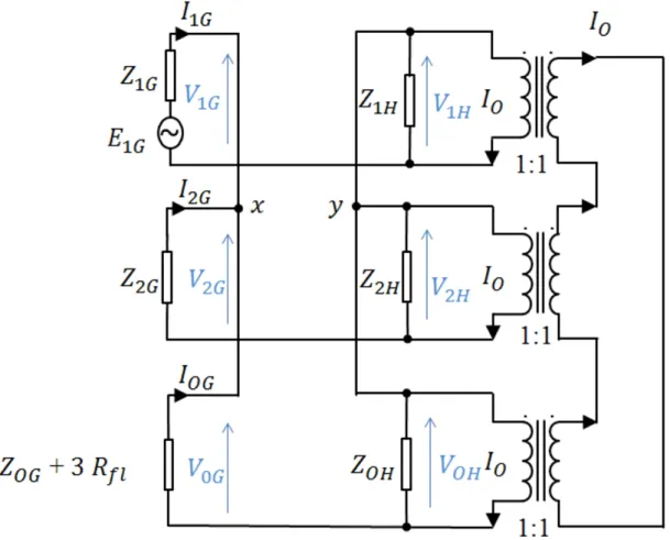
Figure 3.3: Sequence connections diagram from Blackburn(1993).
with the addition of three times the earth fault impedance in series with the source zero
sequence impedance. The earth fault impedance was multiplied by three to allow for
the fact that the sequence network is a single phase representation, however all three
phases of zero sequence current flow through the earth fault impedance (Horowitz &
Phadke 2008).
Blackburn used the labelling of the upstream network with a subscript G and the
downstream network with a subscript H. Blackburn also used the subscripts 1, 2, and
0 to represent the positive, negative and zero sequence impedances respectively. The
following equations are required in the function code to correctly assign the network
impedances to the Blackburn method;
Z1G = Zs+P U +ZsL+P U (3.19)
Z2G = Zs−P U +ZsL−P U (3.20)
Z0G = Zs0P U +ZsL0P U + 3Rf lP U (3.21)
Z1H = ZlL+P U +ZL+P U (3.22)
Z2H = ZlL−P U +ZL
−
P U (3.23)
Z0H = ZlL0P U +ZL0P U (3.24)
Once these assignments have been made the Blackburn equations can be implemented
without modification. The Blackburn method consists of 9 equations as follows;
Zx = Z1H(Z1G+ 2∗Z0G+ 3∗Z0H) +Z0H(Z0G−Z1G) (3.25) Zy = Z2H(2 + 2Z0G) +Z0H(Z1G+Z2G+Z0G+ 6Z2H) (3.26) I1H =
−V s×Zy
Zx(Z1G+Z2H) +Zy(Z1G+Z1H)
(3.27)
I2H = −I1H × Zx
Zy (3.28)
I0H =
−(I1H ×Z1H)−(I2H ×Z2H) Z0H
(3.29)
I0 = −(
1
3 ×I1H + 1
3×I2H + 1
3 ×I0H) (3.30)
I1G = −I1H −I0 (3.31)
I2G = −I2H −I0 (3.32)
These equations are implemented in the Matlab function funcBBL.m to calculate the
positive, negative, and zero sequence currents that flow under fault conditions. The
Matlab function funcBBL.m is included in Appendix B, Section B.2.
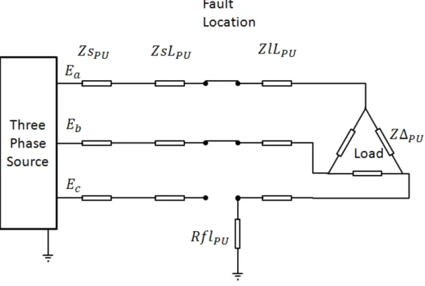
3.1.3 Deriving the Simplified (Phase to Phase to Ground Fault) Model
Figure 3.4: Schematic of three phase Source Isolated Earth Fault.
As mentioned in the literature review this model was derived and not found in peer
reviewed literature. This method was included in this thesis so that the results from
this method can be validated against the peer reviewed methods.
This method relies on the circuit reduction of the Source Isolated Earth Fault schematic
diagram to a phase to phase to ground fault model. The phase to phase to ground fault
is a common fault, and sequence diagrams have been established for the solution of fault
currents under this fault condition (Horowitz & Phadke 2008).
Figure 3.4 shows the schematic diagram of the Source Isolated Earth Fault. Any phase
ZsP U is the source impedance (on the common base). This line may have different positive, negative and zero sequence impedancesZs+P U, Zs−P U, Zs0P U respectively. ZsLP U is the impedance of the line on the source side of the fault (on the com-mon base). This line may have different positive, negative and zero sequence
impedances ZsL+P U, ZsL−P U, ZsL0
P U respectively.
ZlLP U is the impedance of the line on the load side of the fault (on the common base). This line may have different positive, negative and zero sequence impedances
ZlL+P U, ZlL−P U, ZlL0P U respectively.
Z∆P U is the impedance of the load (on the common base). The load may have dif-ferent positive, negative and zero sequence impedances Z∆+P U, Z∆−P U, Z∆0P U re-spectively.
Rf lP U is the impedance of the fault (on the common base).
Figure 3.5: Fault schematic of Source Isolated Earth Fault with star equivalent load impedance.
The first step in simplifying the circuit shown in Figure 3.4 was to convert the delta
the impedance can be calculated from the load current and power factor to find an
equivalent star connected impedance for the load.
The results of the delta to star conversion are shown in Figure 3.5. In this figure the
star equivalent per-phase impedance of the load is labelled ZLP U. Note that the star
connected load does not have an earthed star point.
With the load in a star configuration, the impedances upstream of the fault location
can be summed as they are in series, and the downstream impedances can be summed
also as they are also in series.
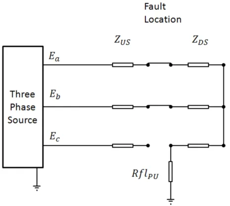
The summed upstream impedances are labelled ZU S, and the summed downstream
impedances are labelled ZDS, in Figure 3.6.
Figure 3.6: Fault schematic reduced by series addition.
Figure 3.6 shows a circuit that is similar to a phase to phase to ground fault. Figure 3.7
shows the phase to phase to ground equivalent diagram for the Source Isolated Earth
Fault for comparison.
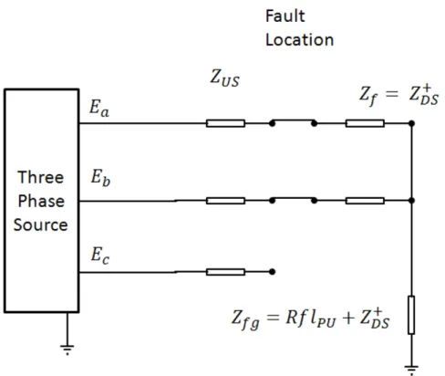
The conversion of the Source Isolated Earth Fault into the equivalent phase to phase
so-Figure 3.7: Fault schematic reduced to phase to phase to ground equivalent.
lution that is relatively simple compared with the Burgess and Blackburn solutions.
The solution employed will be the phase to phase to ground method using sequence
components (Horowitz & Phadke 2008).
In the Matlab script developed for this thesis, the load impedance was calculated in
the star equivalent in the first instance, so the delta to star conversion is not necessary
in the function used in this case.
ZU S = ZsP U +ZsLP U (3.34)
ZDS = ZlLP U +ZLP U (3.35)
Zf = ZDS+ (3.36)
Zf g = Rf lP U +ZDS+ (3.37)
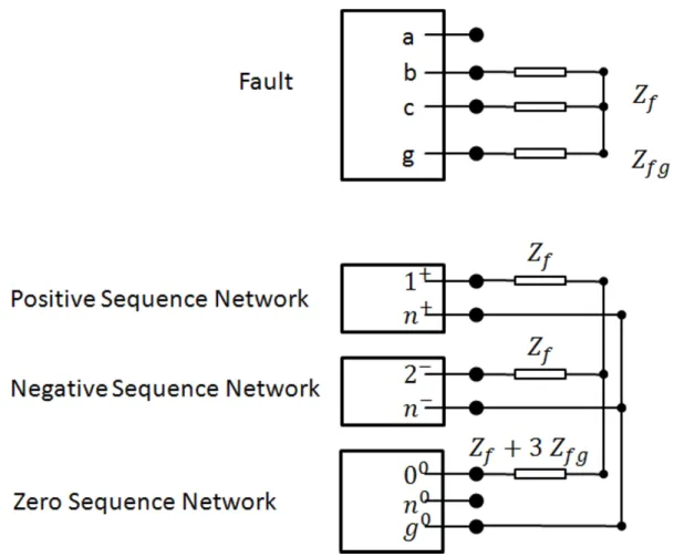
Horowitz (2008) documents the sequence connections for a phase to phase to ground
fault as shown in Figure 3.8. From Figure 3.8 the formulas for calculating the sequence
Figure 3.8: Sequence network connections diagram for phase to phase to ground faults.
active source, it must feed the other two networks in parallel.
ZT otal = ZU S++Zf +
(ZU S−+Zf)(ZU S0+Zf + 3Zf g) (ZU S−+Z
f) + (ZU S0+Zf + 3Zf g)
(3.38)
The positive sequence current must therefore be the supply voltage divided by the total
impedance.
I+ = V s
ZT otal (3.39)
As the two other networks are in parallel, they share the current with the lowest
impedance network drawing the most current.
I− = −I+× (ZU S
0+Z
f + 3Zf g)
(ZU S−+Zf) + (ZU S0+Zf + 3Zf g)
(3.40)
I0 = −I+× (ZU S
−+Z
f) (ZU S−+Z
f) + (ZU S0+Zf + 3Zf g)
These equations are implemented in the Matlab function funcPPE.m to calculate the
positive, negative, and zero sequence currents that will flow under fault conditions. The
Matlab function funcPPE.m is included in Appendix B, Section B.10.
3.1.4 Line Capacitances Added to Models
Line capacitance can be included in the model of a line impedance in various ways.
For the analysis in this thesis it was assumed that the nominal-Π method (Grainger
& Stevenson 1994) is adequate. It was noted that a similar method was applied in
Burgess (2011).
To ensure consistency across the models in this thesis a similar method was employed
by all of the models.
Figure 3.9: Nominal Π circuit of a medium length transmission line.
Figure 3.9 shows a method for the application of line capacitance to a model of a
medium length transmission lines (Grainger & Stevenson 1994).
The schematic circuit for the Source Isolated Earth fault has two line impedances in
series with the load. In this case the impedances of the capacitances can be
com-bined. As the capacitance at the beginning of the first line was in parallel with the
source in the positive sequence network and shorted in the negative and zero sequence
and downstream impedances by applying the series and parallel combinations of those
impedances as appropriate.
Figure 3.10: Circuit simplification to include line capacitance.
Figure 3.10 illustrates the simplification of the line impedances to include the line
ca-pacitance of the lines. New models were created to include the effect of line caca-pacitances
in each model. The method utilised to include the effect of line capacitance was the
same in each case to maintain consistency. The function name of these new models
are similar to before with a suffix of WLC added to each function name to signify that
they calculated the results With Line Capacitance.
These functions appear in Appendix B, funcBBLWLC.m is in Section B.3,
3.1.5 Single Phase Model
Analysis carried out thus far in this thesis has been on three phase networks. Single
phase network is also commonly employed, by utilising two wires only of the three phase
network. Single phase is often used for spurs in lightly loaded areas. Single phase is
utilised on the extremities of feeders. For complete coverage of distribution feeders,
analysis of the source isolated earth fault would then also require analysis of the two
wire single phase condition.
The single phase model was developed following the method developed in section 3.1.3
of this thesis. The fault schematic was reduced to the equivalent of a single phase to
ground fault. The known solution (Horowitz & Phadke 2008) for a single phase to
ground fault was then used to solve for the fault currents.
Figure 3.11: Single phase network schematic.
Figure 3.11 shows the schematic for a normal single phase network. Single phase
network can be comprised of any two phases from a three phase system. Phases A and
Figure 3.12: Single phase Source Isolated Earth Fault schematic.
Figure 3.12 shows the schematic diagram of the faulted system. In this case the C phase
is shown faulted for ease of drawing. The single phase network is simpler to understand
(than the three phase circuit) as the resulting circuit is a series circuit of all impedances
as shown in Figure 3.12 . In Figure 3.13 the impedances are separated into the upstream
and downstream impedances as for the three phase network for consistency across the
Figure 3.13: Fault schematic reduced to the equivalent of a phase to ground Fault.
Figure 3.13 shows the circuit reduction necessary for the single phase model. The
impedances are collected into the upstream impedance, the downstream impedance
and the fault impedance.
ZU S = ZsP U +ZsLP U (3.42)
ZDS = ZlLP U (3.43)
ZF = Zca+ +ZlL+P U +Rf lP U+ (3.44)
Horowitz (2008) documents the sequence connections for a phase to ground fault as
Figure 3.14: Sequence network connections diagram for phase to ground faults.
From Figure 3.14 the formulas for calculating the sequence current can be created. As
the positive sequence network was the only network with an active source it must feed
the other two networks in series with three times the fault impedance.
ZT otal = ZU S+ +Z
+
DS+Z
−
U S+Z
−
DS+ZU S0 +ZDS0 + 3ZF (3.45)
As the sequence impedances are connected in series, all sequence currents must therefore
be equal to the supply voltage divided by the total impedance.
I+ =I− =I0 = V s
ZT otal (3.46)
These equations are implemented in the Matlab function funcSPE.m to calculate the
positive, negative, and zero sequence currents that will flow under fault conditions. The
3.2
Sensitivity Analysis
The sensitivity analysis was performed to carry out two important checks;
1. To test each variable (factor) that was used in the calculation of the Source
Isolated Earth Fault, to ascertain which of the factors were the most significant
in determining the level of earth fault current resulting from this type of fault.
2. To ensure that the derived (phase to phase to ground) model provides a reasonable
estimation of the fault in all tested situations.
The sensitivity analysis was considered more rigorous testing than the case study carried
out in chapter 4 of this thesis, as the sensitivity analysis compared results across many
points whereas the case study was only carried out on 1 scenario. The sensitivity
analysis compared results across all three models for more than 4000 scenarios.
The procedure for the sensitivity analysis was to select a fault scenario, and vary each
of the input factors to the functions from 0.2 to 10 times the chosen values and monitor
the results from each of the functions. The functions will be compared with each other
to check that the models give similar results in each case, and also the effect of varying
each factor will be monitored to ascertain which of the factors has the most effect on
the results.
The One Factor at A Time (OFAT) (Czitrom 1999) testing will be used to identify the
most significant factors in the calculation methods. Further testing will be undertaken
as designed experiments on the significant factors to test for any adverse effects of
varying multiple factors at a time.
The Matlab script built to perform the OFAT testing is SensitivityAnalysis.m it is
included in Appendix B, Section B.17.
3.2.1 OFAT Testing
The OFAT testing requires a starting point for all of the calculations. A starting point
for each of the input variables. The chosen factors are listed here with an explanation
of the choice of the starting point, and a graph of the results.
OFAT Results for Pre-Fault Voltage
The nominal source voltage was represented by a source voltage of 1 PU. This was
the value chosen for the starting point of the OFAT testing. It was expected that the
variation of voltage will create a linear characteristic curve.
Figure 3.15: OFAT results for pre-fault voltage.
The results of varying the source voltage from 0.2PU to 10 PU are shown in Figure
3.15.
As expected the results of all three methods were similar. Analysis of the results found
that the maximum statistical variance between the models was 0.58% when compared
to the Burgess method.
voltage that supplies a fixed circuit of impedances. The resultant curve approximated
a straight line and indicated that the system followed Ohms law. The applied voltage
of a distribution network is not likely to vary significantly as in this test. The variation
of voltage was dropped from further testing.
Source Impedance
The source impedance chosen for the OFAT testing was the same source impedance as
for the case study. This source impedance was supplied by the planning department of
Essential Energy (Gallaher & Arnull 2013) and therefore was considered realistic. The
variation of the source impedance during the OFAT testing provided insight into the
effect of placing the fault models at different locations in the network.
Figure 3.16: OFAT results for source impedance
The results of varying the source impedance are shown in Figure 3.16. As expected
the results of all three methods were similar. Analysis of the results found that the
maximum statistical variance between the models was 0.06% when compared to the
The results showed that varying the source impedance had very little effect on the fault
current in this type of fault, with a variation of only 0.03 Amperes across the entire
field of results for this testing application. This was due to the source impedance being
very small in comparison to the other network impedances. The dominant factors were
discovered elsewhere.
Source impedance was not considered to be an important factor in analysing this type
of fault. This factor was not tested in the second stage of testing.
Network Line Impedances
The network line impedances were carefully selected to allow for a wide range of valid
feeder lengths. Feeders vary in length from short CBD feeders to long rural feeders.
The selection of the network impedances were based on impedances provided by the
planning department of Essential Energy (Gallaher & Arnull 2013). The provided line
impedances provided the positive and zero sequence impedances of the lines, negative
sequence impedances were assumed to be the same as the positive sequence impedances.
The OFAT testing allowed for a maximum feeder length of 440km, and using an equal
amount of the conductor impedances provided. The starting point of the feeder model
for the OFAT testing used 8 km of each of the provided impedances for 7/2.50AAAC,
7/3.00AAAC, 7/3.75AAAC, 7/4.50AAAC and 19/3.75AAAC conductor. This allowed
for the unaltered model to model a fault half way along an 80km (short) feeder, with
an equal mix of conductors. The maximum feeder length during OFAT testing was
440km, with one of the impedances at 40km and the other at 400km. This tested the
effects in long feeders, short feeders and with the fault at varied locations along the
Figure 3.17: OFAT results for upstream network impedance
The results for OFAT testing of the Upstream Network impedance is summarised in
Figure 3.17. As expected the results of all three methods were similar. Analysis of
the results found that the maximum statistical variance between the models was 0.06%
when compared to the Burgess method.
The variation of the upstream network impedance had a noticeable effect on the
re-sults, with a variation of 5.86 Amperes across the entire field of results for this testing
application.
This was due to the upstream network impedance being significant, compared to the
other network impedances. This was identified as one of the dominant factors in
de-termining the level of fault current. This factor was tested further in the next stage of
Figure 3.18: OFAT results for downstream network impedance
The results for OFAT testing of the downstream network impedance is summarised in
Figure 3.18. As expected the results of all three methods were similar. Analysis of
the results found that the maximum statistical variance between the models was 0.06%
when compared to the Burgess method.
The variation of the downstream network impedance had a noticeable effect on the
results, with a variation of 6.4 Amperes across the entire field of results for this testing
application.
This was due to the downstream network impedance being significant, compared to
the other network impedances. This was identified as one of the dominant factors in
determining the level of fault current. This factor was tested further in the next stage
Network Line Capacitances
In a similar way to the line impedances the line capacitance was provided in a dictionary
of conductors for the OFAT testing. The line capacitance used was for more than just
the direct path from the source to the fault on the source side, as the capacitance
of other lateral branches is also present. In a similar way the downstream network
capacitance includes the capacitance of the lateral spurs as well as the direct path to
the end of the feeder.
Figure 3.19: OFAT results for upstream network capacitive reactance..
The results for OFAT testing of the upstream network capacitance is summarised in
Figure 3.19. As expected the results of all three methods were similar. Analysis of
the results found that the maximum statistical variance between the models was 0.14%
when compared to the Burgess method.
The variation of the upstream network capacitance did not have a noticeable effect on
the results, with a variation of 1.55 Amperes across the entire field of results for this
This was due to the upstream network capacitance being less significant than the other
network impedances. This was not identified as one of the dominant factors in
deter-mining the level of fault current. This factor was not tested further in the next stage
of testing.
Figure 3.20: OFAT results for downstream network capacitive reactance.
The results for OFAT testing of the downstream network capacitance is summarised
in Figure 3.20. As expected the results of all three methods were similar. Analysis of
the results found that the maximum statistical variance between the models was 0.16%
when compared to the Burgess method.
The variation of the downstream network capacitance did not have a noticeable effect
on the results, with a variation of 1.59 Amperes across the entire field of results for this
testing application.
This was due to the downstream network capacitance being less significant than the
other network impedances. This was not identified one of the dominant factors in
determining the level of fault current. This factor was not tested further in the next
Downstream Load Impedance
The downstream load impedance selected for OFAT testing was chosen to correspond
with 50 A load current beyond the fault location. This value was chosen to allow the
OFAT testing to test the range of 5 to 250A of load current beyond the fault location.
Figure 3.21: OFAT results for downstream load impedance.
The results for OFAT testing of the downstream load impedance is summarised in
Figure 3.21. As expected the results of all three methods were similar. Analysis of
the results found that the maximum statistical variance between the models was 0.12%
when compared to the Burgess method.
The variation of the downstream load impedance had a noticeable effect on the
re-sults, with a variation of 30.6 Amperes across the entire field of results for this testing
application.
This was due to the downstream load impedance being significant, compared to the
other network impedances. This was identified as the dominant factor in determining
Fault Impedances
As the Burgess model allowed for a source side fault as well as the load side (source
isolated) fault, two fault impedances were passed to the functions. As the scope of
this thesis only includes the load side (source isolated) earth fault, the source side fault
impedance was assumed to be infinity. Infinity was not possible to represent directly
in the code, so the source side fault impedance was set to 1 E99 which was considered
sufficiently large to represent the impedance of an open circuit even at the extremes of
OFAT testing. No results of the OFAT testing are provided for the source side fault
impedance, as it is not within the scope of this thesis.
For the load side (source isolated) fault impedance, a value of 30 Ohm was selected in
accordance with Essential Energy policy (Essential Energy 2012). The resulting OFAT
range of fault impedances tested was 6 to 300 Ohms.
Figure 3.22: OFAT results for fault impedance.
The results for OFAT testing of the fault impedance is summarised in Figure 3.22. As
expected the results of all three methods were similar. Analysis of the results found
to the Burgess method.
The variation of the fault impedance had a noticeable effect on the results, with a
variation of 9.2 Amperes across the entire field of results for this testing application.
This was due to the fault impedance being significant, compared to the other network
impedances. This factor was tested further in the next stage of testing.
Summary of Results of OFAT Testing
OFAT testing was employed to identify the dominant factors in the Source Isolated
Earth Fault, and to confirm the methods employed provide similar results. This
con-firmed both the application of the methods to the task and the coding of those methods
to be suitably accurate to estimate the earth fault current developed during one of these
faults.
Table 3.2: Summary of OFAT results.
Source Source US US US DS DS DS DS
Voltage Z Line Cap Fault Line Cap Load Fault
Z Z Z Z Z Z Z
Variation 137.3 0.03 5.86 1.55 0 6.39 1.59 30.63 9.16
(A)
Max Error 0.58 0.06 0.06 0.14 0.06 0.06 0.16 0.12 0.08
(%)
Ranking Not 7 4 5 8 3 6 1 2
Ranked
Note: US = Upstream, DS = Downstream, Z = Impedance, Cap = Capacitive
The results of the OFAT testing are summarised in Table 3.2.
The maximum statistical variance between the methods was 0.58%. The simplified
method was considered to be an adequate means of estimating the earth fault current
The OFAT testing allowed the factors to be ranked in order of significance. The most
significant factor was found to be the load impedance beyond the fault location. The
four most significant factors were concentrated on in a second stage of analysis. The
second stage of analysis carried out experiments to determine any interaction between
the significant factors.
3.2.2 Designed Experiments
Designed experiments (Czitrom 1999) provide a means to examine the interaction
be-tween factors in complex models. OFAT testing concentrated on varying all factors, one
at a time over a large range of input possibilities to find the significant factors in the
models. The designed experiments vary multiple factors at the same time to identify if
there are any interactions between the input factors that produce unexpected results.
Figure 3.23: Source Isolated Earth Fault schematic.
As many factors were manipulated together a lesser variation in the input factors was
allowed. This was due to the added complexity in calculating and displaying the results.
in the designed experiments.
Figure 3.23 shows the schematic of the source isolated earth fault. In this testing regime
the focus was on the following four major factors (All in PU on the common base);
1. ZsLP U was the impedance of the line on the source side of the fault.
2. ZlLP U was the impedance of the line on the load side of the fault.
3. ZLP U was the impedance of the load.
4. ZlLP U was the impedance of the line on the load side of the fault.
For the designed experiments the multiplication factors varied from 1 to 2 in steps of
0.1 all factors were varied and the results for all possible combinations were recorded
and graphed. This created a 4 dimensional array.
Displaying the 4 (mathematical) dimensions on a three dimensional graph was not
easy. To build toward this three dimensional data was built on 10 separate graphs.
Figure 3.24: Combined graph of 10 variations in upstream, downstream, load and fault impedances.
Figure 3.24 shows the combined results of the multi-variable analysis. The results were
grouped by colour for the load impedance factor. In each group the fault impedance
factor varied from 1 to 2 in ten steps.
The results trivially proved that higher impedance draws less current. The load impedance
remained the dominant factor in the multi-variable analysis. The combined graph
showed no adverse interactions between factors.
The Matlab script built to perform the designed experiments is
MultiVariableAnaly-sis.m it is included in Appendix B, Section B.16.
3.2.3 Code Profiling
Matlab provides built in code profiling functions. Profiling allows the user to view the
total time that the code spends in each function. The first attempts at profiling the
results were erratic due to the relative short time for the processes to occur on modern
computers.
Figure 3.25: Matlab profiler results.
To stabilise the profiling data The Matlab program was restricted to use only one
processor (according to the method provided in MATLAB Help) and the process was
run 1 million times so that adequate data could be gathered. All other non-essential
software was shut down on the workstation during the profile test.
Figure 3.25 shows typical results obtained from running the source isolated earth
fault functions 1 million times on the same input data. The functions of interest are
funcBurgessWLC (137.935 s), funcBBLWLC (22.751 s) and funcPPEWLC (11.343 s).
The profiling results show that the simplified method was significantly faster than the
Figure


Related documents