Thesis by
Ganesh Subramanian
In Partial Fulfillment of the Requirements for the Degree of
Doctor of Philosophy
CA L IF
O
RN
IA
INST
ITUTE OFT
E
C
H
N
O
L
O
G
Y 1891
California Institute of Technology Pasadena, California
2002
c
2002
Acknowledgements:
To begin with, I wish to acknowledge my advisor, John Brady, for his encourage-ment and support through this odyssey. My academic discussions with him have always been illuminating and his acute physical insight will continue to be a source of inspiration. I also thank my group: Mike and Sundar for guiding me through the initial days of uncertainity, and Ileana, in particular, for keeping my spirits up and the flame burning as the journey was nearing its end.
Among people at Caltech, Murtuza, Amit and Anu have been very helpful at different stages in my PhD. I am indebted to Prakash and Vidya for inculcating in me, a love for Indian classical music. Outside of Caltech, my friends Satish and Aravind have been pillars of support. Satish especially has always been a willing confidant; his short stay in California is one I will always cherish.
Abstract
This work analyses the role of small but finite particle inertia on the microstructure of sus-pensions of heavy particles subjected to an external flow. The magnitude of particle inertia is characterized by the Stokes number (St), defined as the ratio of the inertial relaxation time of a particle to the flow time scale. Fluid inertia is neglected so that the fluid motion satisfies the quasi-steady Stokes equations. The statistics of the particles is governed by a Fokker-Planck equation in position and velocity space. For small St, a multiple scales formalism is developed to solve for the phase-space probability density of a single spherical Brownian par-ticle in a linear flow. Though valid for an arbitrary flow field, the method fails for a spatially varying mass and drag coefficient. In all cases, however, a Chapman-Enskog-like formulation provides a valid multi-scale description of the dynamics both for a single Brownian particle and a suspension of interacting particles. For long times, the leading order solution simplifies to the product of a local Maxwellian in velocity space and a spatial density satisfying the Smoluchowski equation. The higher order corrections capture both short-time momentum relaxations and long-time deviations from the Maxwellian. The inertially corrected Smolu-chowski equation includes a non-Fickian term at O(St).
Contents
1 Introduction 1
Bibliography 8
2 Multiple scales analysis of the Fokker-Planck equation for a single
Brown-ian particle in simple shear flow 11
2.1 Introduction . . . 11
2.2 Problem formulation . . . 14
2.3 Brownian motion in simple shear flow . . . 19
2.3.1 Exact solution . . . 20
2.3.2 Multiple scales analysis . . . 24
2.4 Comparison of exact and multiple scales solutions . . . 36
2.4.1 Multiple scales solution for a Maxwellian initial condition . . . 36
2.4.2 Multiple scales solution for a delta function initial condition . . . 42
2.4.3 The athermal limit . . . 45
2.5 Conclusions and discussion . . . 48
3.2 Equivalence of the Chapman-Enskog and multiple scales formalisms for a single
Brownian particle in an external flow . . . 55
3.3 Chapman-Enskog method for a configuration dependent drag force in one di-mension . . . 59
3.4 Chapman-Enskog method for inertial suspensions . . . 64
3.4.1 Introduction . . . 64
3.4.2 Problem formulation . . . 67
3.4.3 Multiple scales analysis . . . 71
3.4.4 Higher order inertial corrections . . . 88
3.5 Conclusions . . . 91
Bibliography 93 4 Trajectory analysis for inertial non-Brownian suspensions: In-plane trajec-tories 95 4.1 Introduction . . . 95
4.2 Equations for particle trajectories . . . 97
4.3 Nature of inertial velocity corrections for small Stokes numbers . . . 103
4.4 Relative in-plane trajectories of two spheres in simple shear flow . . . 109
4.4.1 Open trajectories with initial offsets much greater thanO(St12) . . . . 115
4.4.2 The effect of hydrodynamic coupling on the in-plane gradient displace-ment . . . 127
4.4.3 In-plane Limiting trajectory . . . 130
4.4.5 Calculation of in-plane self-diffusivity in the velocity gradient
direc-tion (Dzzip) . . . 140
4.4.6 Behavior within the limiting trajectory . . . 147
Bibliography 160 5 Trajectory analysis for inertial non-Brownian suspensions: Off-Plane tra-jectories 163 5.1 Introduction . . . 163
5.2 Relative off-plane trajectories . . . 166
5.2.1 Off-Plane open trajectories . . . 166
5.2.2 Off-plane spiralling trajectories . . . 170
5.3 Perturbation analysis for off-plane trajectories . . . 176
5.3.1 Open trajectories with initial gradient offsets much greater thanO(St12).178 5.3.2 Open trajectories with initial gradient offsets ofO(St12) . . . 186
5.3.3 Far-field analytical expressions for lateral displacements ∆z and ∆x . 199 5.3.4 Scaling of self-diffusivities in the velocity gradient (Dzz) and vortic-ity (Dxx) directions . . . 209
5.4 Comparison with direct numerical simulation of pair trajectories . . . 212
5.5 Microstructure and rheology . . . 216
Bibliography 219
6 Conclusions 222
A Appendices for Chapter 2 226
A.1 Free Brownian motion . . . 226
A.1.1 Exact solution . . . 227
A.1.2 Multiple scales analysis . . . 229
A.1.3 Failure of the naive multiple scales scheme . . . 233
A.2 Two-time-scale expansions of the exact solutions . . . 235
A.3 Inertial corrections to equation (2.36) for b(0)m,n . . . 240
A.4 Identity of exact and multiple scales solutions of section 2.4.2 . . . 244
A.4.1 Identity of leading order solutions . . . 244
A.4.2 Identity of O(St)velocity-dependent corrections . . . 250
A.5 Solution to the inhomogeneous Smoluchowski equation . . . 259
A.5.1 Green’s function for the Smoluchowski equation . . . 259
A.5.2 A Green’s function identity . . . 260
B Appendices for Chapter 3 263 B.1 TheO(St) Chapman-Enskog solution, ¯PM(1), for general M . . . 263
C Appendices for Chapter 4 266 C.1 TheO(1) andO(St) velocity fields . . . 266
C.2 O(St) solution in the outer layer O1 . . . 270
C.3 Non uniform nature of theO(St) corrections for zero-Stokes closed trajectories 272 C.4 In-plane open trajectories with initial offsets ofO(Stβ) (0< β≤1/2) . . . . 274
List of Figures
1.1 Parameter plot delineating the domain of validity (shaded region) of our work. 4
2.1 Iso-probability contours in simple shear flow for St≥0. . . 33
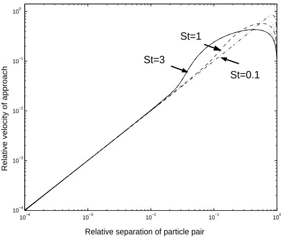
4.1 One-dimensional approximation for the relative velocity of approach for two spheres. Initial condition: u0 = 5, y0 = 1. . . 108
4.2 One-dimensional approximation for the relative approach velocity of two spheres. Initial condition: u0= 0.1, y0= 1 . . . 108
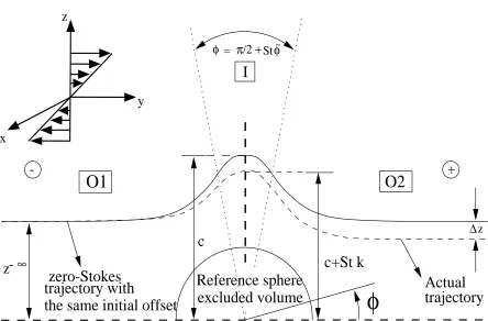
4.3 Finite Stopen trajectory with O(1) initial offset. . . 115
4.4 Stresslet velocity field induced by a sphere in shear flow. . . 128
4.5 Finite Stlimiting trajectory in the plane of shear. . . 131
4.6 The critical offset (mc1St12) values obtained from numerical integration of the in-plane trajectory equation (4.25) are plotted as a function of St12. . . 136
4.7 Tracer particle (darker shade) undergoing a random walk due to successive uncorrelated pair-interactions. . . 141
4.8 Trajectory spiralling into the limit cycle for St= 0.2. . . 154
4.9 Trajectory spiralling into the limit cycle for St= 0.2. . . 154
4.10 Trajectory spiralling out onto the limit cycle forSt= 0.2. . . 155
4.11 Trajectory spiralling into the limit cycle forSt= 0.1. . . 156
4.12 Trajectory spiralling into the limit cycle forSt= 0.1. . . 156
4.13 Trajectory spiralling out onto the limit cycle forSt= 0.1. . . 157
4.15 Trajectory spiralling into the limit cycle forSt= 0.02. . . 158
4.16 Trajectory spiralling out onto the limit cycle forSt= 0.02 . . . 158
4.17 Phase plane of trajectories forSt= 0 in simple shear flow. . . 159
4.18 Phase plane of trajectories for finite Stin simple shear flow. . . 159
5.1 Zero Stoff-plane open trajectory forx−∞= 0.5 and z−∞= 0.15 . . . 164
5.2 Off-Plane open trajectory forx−∞= 0.5,z−∞= 0.15 and St= 0.1 . . . 164
5.3 Off-Plane closed orbit starting through (x, y, z)≡(0.1,−3,0) . . . 165
5.4 Inward spiralling off-plane trajectory starting from (x, y, z) ≡(0.1,−3,0) for St= 0.1. . . 165
5.5 Axisymmetric separatrix envelope enclosing closed orbits at St= 0. . . 167
5.6 ModifiedSt spiralling trajectories within the modified separatrix envelope. . 171
5.7 Geometric relation between gradient and vorticity displacements . . . 185
5.8 Off-Plane inertial trajectory withO(St12) initial gradient offset. . . 186
5.9 Off-Plane open trajectory forx−∞= 0.5 andz−∞= 0.5. . . 194
5.10 Limiting off-plane open trajectory forx−∞= 0.5 andz−∞= 0.12. . . 195
5.11 Off-plane open trajectory forx−∞= 1.5 andz−∞= 0.5. . . 196
5.12 Off-plane open trajectory forx−∞= 1.5 andz−∞= 0.15. . . 196
5.13 Limiting off-plane open trajectory forx−∞= 1.5 andz−∞= 0. . . 197
5.14 Spiralling off-plane trajectory starting from (x, y, z)≡(1.8,−1,0). . . 197
5.15 Off-plane trajectory starting from (x, y, z) ≡(2,−0.5,0) and spiralling off to infinity. . . 198
List of Tables
4.1 (∆z)inplane values with and without theU· ∇xΩcontribution: St= 0.1. . . . 129
4.2 Comparison of theoretical and numerical values of the critical offset in the shearing plane. . . 135
4.3 Comparison of numerical and analytical values, and the far-field approxima-tion (4.55) of (∆z)inplane forSt= 0.1. . . 140
4.4 Comparison of analytical and numerical values of the in-plane diffusivity for different Stokes numbers. . . 147
5.1 ∆x values forx−∞= 0.2 andz−∞ ranging from 5 to 0.1; St= 0.1,0.01. . . . 184
5.2 ∆x values forx−∞= 1 and z−∞ ranging from 5 to 0.1; St= 0.1,0.01. . . 184
5.3 Limiting offsets for off-plane trajectories for small x−∞; St= 0.1,0.01. . . 191
5.4 Values of ∆z forx−∞= 1.5 and 5,z−∞ranging from 5 to 0.1;St= 0.1,0.01. 193 5.5 Comparison of numerical and the far-field approximation (5.42) of ∆x in the limit x−∞, z−∞1 forSt= 0.1. . . 201
5.6 Comparison of numerical values and the far-field approximation (5.43) of ∆z in the limit x−∞, z−∞1 forSt= 0.1. . . 204
5.7 Comparison of numerical values and the analytical approximation (5.44) for ∆x in the limitx−∞1, z−∞= 0 for St= 0.1. . . 206
5.8 ∆x and ∆z values forx−∞= 0 and z−∞ ranging from 5 to 0.1. . . 214
5.9 ∆x and ∆z values forx−∞= 0.2 andz−∞ ranging from 5 to 0.1. . . 214
Chapter 1
Introduction
A suspension is a multiphase system where the dispersed phase comprising solid particles is suspended in a fluid medium. Suspensions are important in a variety of natural and in-dustrial settings including landslides, drilling fluids, fluidized beds, etc; a great majority of processes in the chemical industry entail the handling and transport of multiphase materials. The suspended particles in these systems interact through hydrodynamic, interparticle and Brownian forces. The interplay between these forces leads to a macroscopic flow behavior that is complex and often strikingly different when compared to a Newtonian fluid like water. Indeed, it is now known that concentrated suspensions cannot be treated using a classical Newtonian formulation with an effective viscosity. Even with a Newtonian suspending fluid, suspensions at high enough particle concentration exhibit pronounced non-Newtonian be-havior with normal stress differences and a shear-rate-dependent viscosity (Jeffrey & Acrivos 1976, GadalaMaria & Acrivos 1980, Singh 2000, Zarraga et al 2000). Thus, an understanding of suspension properties is of great interest both from a fundamental point of view and with regard to enhancing the efficiencies of the aforementioned industrial processes.
sus-pension, an effect that was originally shown for the case of Poiseuille flow (Segre & Silberberg 1962ab, Ho & Leal 1974). Particle inertia leads to the preferential concentration of particles in regions of high strain rate in dilute particle-laden turbulent flows, and this in turn has a significant effect on the fluid phase turbulence (Eaton & Fessler 1994). In general, inertial effects in suspensions have been shown to induce non-Newtonian behavior (Lin et al 1970, Tsao & Koch 1995). Ideally, it is desirable to study the separate roles of particle and fluid inertia in suspension flows. Since the ratio of particle to fluid inertia scales as the ratio of the densities of the respective phases, it is possible to study particle inertia independent of fluid inertial effects for suspensions of heavy particles; for instance, considering 10 micron particles in air (η ∼ 10−5P a.s, ρp/ρf ∼ 1000) and a typical shear rate ∼ 10s−1, one has
St= 0.1 and Re= 10−4. This work considers the role of particle inertia in determining the
microstructure and rheology of heavy suspensions. Inertial forces in the fluid are therefore neglected (Re = 0) and the suspending fluid satisfies the Stokes equations. The statistics of the particles are given by a probability density function that satisfies a Fokker-Planck equa-tion in phase space. A dimensionless measure of particle inertia is the Stokes number (St), defined as the ratio of the inertial relaxation time of a particle to the flow time scale.
Particle inertia is dominant in these cases and the effect of the interstitial (suspending) fluid is often neglected. Interparticle collisions are the main mechanism of momentum transport at high concentrations, and the statistics of the particles are therefore modeled by analogy with a molecular hard-sphere gas, the difference being that the collisions between the macroscopic particles are dissipative (Jenkins & Savage 1983, Lun et al 1984, Jenkins & Richman 1985ab, Campbell 1990). In the last decade, Koch and co-workers have developed a theory for zero Re, finite (but large) Stsuspensions that accounts for the effects of interstitial fluid (Tsao & Koch 1995, Sangani et al 1996).
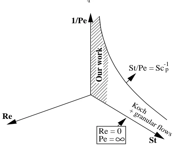
This present work is valid for zero Re, small but finite St, and in addition, we allow for Brownian effects by letting the Peclet number (P e), defined as the ratio of the Brownian diffusion time scale to the flow time scale, be finite. The reason for the latter is that the highP elimit (i.e., strongly sheared suspensions) is known to be singular (Brady & Morris 1997); Brownian diffusion and advection effects balance in asymptotically thin (O(P e−1)) boundary layers near particle-particle contact, and the resulting asymmetry of the boundary layer microstructure leads to persistent non-Newtonian effects that decay very slowly (≈ P e−0.22) asP e→ ∞. Our analysis allows one to investigate the effect of particle inertia (finite St) on this limiting behavior. The domain of validity of our work is shown in Fig 1.1 in the parameter space spanned byRe, St andP e. The ratioSt/P e is independent of the flow and small compared to unity1, implying that Brownian effects need only be considered for small St.
The thesis is divided in two parts. The first part, comprising Chapters 2 and 3, introduces and develops a multiple scales (Chapman-Enskog) formalism to solve the Fokker-Planck equation for small but finite St(and arbitrary P e) in non-equilibrium situations.
1This ratioSt/P e=Sc−1
p , whereScpis the Schmidt number and the subscriptpis used to indicate that
the kinematic viscosity in the definition ofScpis based on the particle density;Scp1 whence the conclusion
+ granular flowsKoch
Our work
Re = 0
Pe =
Re
1/Pe
St
[image:17.612.177.457.55.294.2]St/Pe = Sc
-1pFigure 1.1: Parameter plot delineating the domain of validity (shaded region) of our work.
In Chapter 3, we derive an inertially corrected Smoluchowski equation accurate to O(St) that includes the first effects of particle inertia. The suspension (spatial) microstructure is characterised by the pair-distribution function that satisfies the well-known Smoluchowski equation in the inertialess limit (St = 0). The solution to the corrected equation therefore accounts for changes in the suspension microstructure for finiteSt, thus serving to determine inertial modifications of the suspension flow properties. Chapters 4 and 5 are devoted to applying the formalism in order to obtain explicit results for simple shear flow of a dilute non-Brownian suspension of spherical particles. Each of chapters 2, 3, 4 and 5 have associated appendices that are labeled A, B, C and D, respectively.
particle (τp), the time scale for Brownian diffusion (τD) and the time scale imposed by the
shear flow ( ˙γ−1, ˙γ being the shear rate). The governing Fokker-Planck equation describes the evolution of the probability density on time scales ofO(τp) or longer; for smallSt, it therefore
accounts for both the rapid momentum relaxations in O(τp) and the slower spatial diffusion
processes on time scales of O( ˙γ−1) or O(τ
D). The disparate time scales of momentum and
spatial relaxations motivate the use of a multiple scales method for the problem. However, it is shown that the customary multiple scales procedure (which has been successfully used, for instance, in the analysis of linear and non-linear oscillators to yield amplitude/phase modulated periodic solutions, and for non-linear wave equations to yield similarly modulated travelling wave solutions; see Kevorkian & Cole (1995)) does not work for the Fokker-Planck equation since the independent variables in this case span both position and velocity space, and including only one of the two (as in the naive multiple scales approximation) leads to spurious relaxation terms. We therefore employ a modified version of the formalism originally used by Wycoff & Balazs (1987) for the Kramers equation2; in our case, this entails expanding
the probability density in an infinite series of Hermite functions of the fluctuation velocity, defined as the difference between the velocity of the Brownian particle and the velocity of the ambient simple shear flow at its instantaneous location. The expansion coefficients in the infinite series are found to satisfy Smoluchowski-like equations with inertial corrections at successive orders inSt. The coefficient of the zeroeth order Hermite function represents the number density and satisfies a corrected Smoluchowski equation containing an off-diagonal diffusive component at O(St).
For a finite St suspension in an external flow, the time scale for momentum re-laxations becomes configuration dependent on account of hydrodynamic interactions, and
2The Fokker-Planck equation in one dimension is better known as Kramers equation in the physics literature
the multiple scales formalism introduced in Chapter 2 is no longer applicable in its original form (i.e., in the form used for a single particle). In Chapter 3 we formulate a generalized Chapman-Enskog expansion that still shares the same basic structure as the original multi-ple scales formalism, but accounts for the commulti-plex form of the momentum relaxations in a suspension. The expansion of the probability density is now in terms of tensorial Hermite functions; the coefficient of the zeroeth order term, however, still represents the number den-sity, and we derive a corrected Smoluchowski equation for the same, including the O(St) inertial terms. In addition to (expected) corrrections to the leading order velocity field and diffusivities, the equation derived is shown to contain a non-Fickian term at O(St/P e2).
Though applicable only in the limit St 1, the range of validity of the Chapman-Enskog formulation is expected to increase with increase in the particle volume fraction (φ) because, for fixed St, the increase in the suspension viscosity with increasing φ reduces the effective particle inertia.
no net displacement in the transverse direction. Although the zero-Stokes open trajectories support an isotropic distribution, the existence of a region of closed trajectories in simple shear flow leads to an indeterminate pair-distribution function (Batchelor & Green 1972b). A well-posed steady problem can only be obtained by the inclusion of (say) Brownian motion or three-particle interactions. Particle inertia destroys the fore-aft symmetry of the zero-Stokes trajectory space, giving rise to net transverse displacements in the velocity gradient and vorticity directions (of simple shear flow) following each pair-interaction, in turn leading to diffusive behavior for long times. The differing strengths of interaction along the gradi-ent and vorticity directions result in an anisotropic self-diffusivity tensor, the gradigradi-ent and vorticity components of which scale as St2lnStand St2, respectively. Unlike the inertialess limit where the indeterminacy of the rheological problem is related to the dependence of the long-time distribution on the particular initial condition (in the region of closed trajectories), the indeterminacy for finite St arises from the absence of such a long-time limit. For finite Stthe region of closed trajectories is destroyed, but there exists instead a planar limit cycle that acts as a local attractor; the associated basin of attraction has an infinite volume. As a result, (almost) any initial condition3 for long times leads to a progressive accumulation of particles on the attracting cycle, resulting in a temporally growing distribution. As is the case for St= 0, one again needs to include additional mechanisms in order to obtain a well-posed rheological problem.
It is finally noted that notwithstanding use of the corrected Smoluchowski equa-tion derived in Chapter 3, the second part of the thesis comprising Chapters 4 and 5 is more or less self contained and maybe read independently of the first.
3One may obtain a finite long-time pair-distribution function for initial conditions that correspond to a
Bibliography
[1] Batchelor, G.K. & Green, J.T. 1972a The hydrodynamic interaction of two small freely-moving spheres in a linear flow field.J. Fluid Mech. 56, 375-400.
[2] Batchelor, G.K. & Green, J.T. 1972b The determination of the bulk stress in a suspension of spherical particles to O(c2).J. Fluid Mech.56, 401-427.
[3] Brady, J.F. & Bossis, G. 1988 Stokesian dynamics. Ann. Rev. Fluid Mech.20, 111-157.
[4] Brady, J.F. & Morris, J.F. 1997 Microstructure of strongly sheared suspensions and its impact on rheology and diffusion.J. Fluid Mech.348, 103-139.
[5] Campbell, C.S. 1990 Rapid granular flows. Ann. Rev. Fluid Mech.22, 57-92.
[6] Eaton, J.K. & Fessler, J.R. 1994 Preferential concentration of particles by turbulence.
Int. J. Multiphase Flow 20, Suppl. S, 169-209.
[7] Fessler, J.R., Kulick, J.D. & Eaton, J.K. 1994 Preferential concentration of heavy-particles in a turbulent channel flow.Phys. Fluids 6(11), 3742-3749.
[8] GadalaMaria, F. & Acrivos, A., 1980 Shear-induced microstructure in a concentrated suspension of solid spheres.J. Rheol. 24(6), 799-814.
[9] Happel, J. & Brenner, H. 1965 Low Reynolds number hydrodynamics, with special appli-cations to particulate media. Prentice-Hall.
[11] Jeffrey, D.J. & Acrivos, A. 1976 Rheological properties of suspensions of rigid particles.
AIChE J.22(3), 417-436.
[12] Jenkins, J.T. & Richman, M.W. 1985a Grads 13-moment system for a dense gas of inelastic spheres.Arch. Ration. Mech. Anal. 87(4), 355-377.
[13] Jenkins, J.T. & Richman, M.W. 1985b Kinetic-theory for plane flows of a dense gas of identical, rough, inelastic, circular disks.Phys. Fluids 28(12), 3485-3494.
[14] Jenkins, J.T. & Savage, S.B. 1983 A theory for the rapid flow of identical, smooth, nearly elastic, spherical-particles. J. Fluid Mech.130, 187-202.
[15] Kevorkian, J. & Cole, J.D. 1995 Multiple Scale and Singular Perturbation Methods.
Springer-Verlag.
[16] Kim, S. & Karrila, S.J. 1991 Microhydrodynamics: Principles and Selected Applications.
Butterworth-Heinemann.
[17] Kramers, H.A. 1940 Brownian motion in a field of force and the diffusion model of chemical reactions.Physica 7, 284-304.
[18] Kulick, J.D., Fessler, J.R. & Eaton, J.K. 1994 Particle response and turbulence modifi-cation in fully-developed channel flow. J. Fluid Mech. 277, 109-134.
[19] Lin, C.J., Peery, J.H. & Schowalter, W.R. 1970 Simple shear flow round a rigid sphere: inertial effects and suspension rheology. J. Fluid Mech.44, 1-17.
[21] Rouson, D.W.I. & Eaton, J.K. 2001 On the preferential concentration of solid particles in turbulent channel flow.J. Fluid Mech.428, 149-169.
[22] Sangani, A.S., Mo, G., Tsao, H.K. & Koch, D.L. 1996 Simple shear flow of dense gas-solid suspensions at finite Stokes numbers.J. Fluid Mech.313, 309-341.
[23] Segre, G. & Silberberg, A. 1962a Behavior of macroscopic rigid spheres in Poiseuille flow. Part 1. Determination of local concentration by statistical analysis of particle passages through crossed light beams.J. Fluid Mech. 14, 115-135.
[24] Segre, G. & Silberberg, A. 1962b Behavior of macroscopic rigid spheres in Poiseuille flow. Part 2. Experimental results and interpretation.J. Fluid Mech.14, 136-157.
[25] Singh, A. 2000 Rheology of non-colloidal suspensions. PhD Thesis, Indian Institute of Science, Bangalore, India.
[26] Zarraga, I.E., Hill, D.A. & Leighton, D.T. 2000 The characterisation of the total stress of concentrated suspensions of non-colloidal spheres in Newtonian fluids.J. Rheol. 44, 185-220.
[27] Tsao, H.K. & Koch, D.L. 1995 Simple shear flows of dilute gas-solid suspensions. J. Fluid Mech.296, 211-245.
Chapter 2
Multiple scales analysis of the Fokker-Planck
equa-tion for a single Brownian particle in simple shear
flow
2.1
Introduction
The Fokker-Planck equation (also known as the Kramers-Chandrasekhar equation) is the fundamental equation governing the statistics of a Brownian particle in phase space. Re-stricting consideration to position coordinates alone gives a coarser description character-ized by the well-known Smoluchowski equation (Smoluchowski 1915). The derivation of the Smoluchowski equation from the Fokker-Planck equation involves neglecting processes that occur on the scale of the particle inertial relaxation time (τp). It is this separation of time
In this chapter we extend the formalism of Wycoff & Balazs to a Brownian particle in a simple shear flow. The velocity field is given by ushear(y) = ˙γy¯1x, and gives
rise to a nonconservative hydrodynamic force field owing to the vorticity of the imposed flow. Here ˙γ is the shear rate, 1x is the unit vector in the flow direction and ¯y is the coordinate
in the gradient direction. In addition to the inertial (τp) and configurational (τD = a2/D,
where D is the diffusivity) relaxation times, the shear rate introduces a new time scale ˙
γ−1, and the assumption made here is a separation of the inertial and flow time scales. Therefore, the method remains valid for arbitrary relative magnitudes of τD and ˙γ−1, that
is, arbitrary values of the Peclet number P e = ˙γτD. In contrast to equilibrium problems,
the pertinent variable for the Hermite functions (in the expansion of the probability density) is no longer the absolute velocity of the Brownian particle but rather the difference between its absolute velocity and the velocity of the unperturbed flow field at its current location. As it is convected by the flow, the particle can only equilibrate about the instantaneous flow velocity and the ‘equilibrium’ distribution is therefore a local Maxwellian about the ambient flow velocity. The main purpose of this chapter is to develop a consistent multiple time scales scheme for such non-equilibrium problems and to compare explicitly the exact and multiple scales solutions for the case of simple shear flow.
parti-cles are taken into account, for in this case, the corrected Smoluchowski equation governs the effect of the inertia of the particulate phase on suspension microstructure. The limit of vanishing Brownian motion is also of special interest since a non-colloidal, inertialess suspen-sion possesses a symmetric microstructure with a Newtonian rheology. The multiple scales method would enable one to study the effects of inertia on this microstructural symmetry and its consequences for suspension rheology.
on modifications in the procedure necessary when considering hydrodynamically interacting particles.
2.2
Problem formulation
The Fokker-Planck equation for a single particle in shear flow is
∂P ∂t¯ +u·
∂P ∂y +
˙ γy¯ m1x·
∂P ∂u =
6πηa m
∂
∂u ·(uP) + kT
m
6πηa m
∇2uP. (2.1)
Here,P(y,u,¯t)dyduis the probability that the Brownian particle is in the elemental volume [(y,y+dy),(u,u+du)] at time ¯t,mis the mass of the particle,ais its radius,ηis the viscosity of the suspending fluid andT is the absolute temperature. Using the non-dimensionalizations: ¯
t=m/(6πηa)t, y=axand u= ( ˙γa)v, (2.1) becomes
∂P
∂t +Stv· ∂P
∂x = ∂
∂v·(v−y1x)P + 1 P e St∇
2
vP. (2.2)
In equation (2.2), the Stokes number St=mγ/˙ (6πηa) is the ratio of the inertial relaxation time (τp = m/6πηa) to the flow time scale, and is a measure of the inertia of
the Brownian particle, while P e= (6πηa3γ˙)/kT is a measure of the importance of thermal effects. Thus in the limit St 1, we have ˙γ−1 τp, which illustrates the separation of
relaxes so that the particle, in effect, encounters a steady flow field and use of the steady Stokes drag is appropriate on all time scales starting fromτp. In fact, equation (2.1) can also
be written as the equivalent Langevin equation,
mdu
dt =−6πηa(u−γ˙y¯1x) +F
B(t), (2.3)
whereFB(t) is the Brownian force modelled as a delta-correlated white noise with amplitude
determined from the fluctuation dissipation theorem (Chandrasekhar 1954):
hFB(t)i= 0 , hFB(t)FB(t0)i= 2kT(6πηa)δ(t−t0).
The configuration space Smoluchowski equation for a Brownian particle in shear flow corresponding to the Fokker-Planck equation (2.1) is
∂g ∂¯t +
∂
∂y ·( ˙γy¯1xg) =D∇
2
yg , (2.4)
whereg(y,t¯) is the positional probability density at time ¯tandD= kT /(6πηa) is the Stokes-Einstein diffusivity. The Langevin equation of motion equivalent to (2.4) is given by (2.3) with m = 0. When the time ¯t is scaled with the shear rate (representative of the slower spatial relaxation processes), the non-dimensional Smoluchowski equation becomes
∂g ∂t +
∂
∂x(yg) = 1 P e∇
2
xg. (2.5)
our goal to obtain corrections to (2.5) for small Stokes numbers.
The multiple scales formalism is suited to the description of dynamical systems characterised by concurrent processes occurring on widely separated time scales. The evolu-tion of the momentum and spatial coordinates of a Brownian particle in shear flow for small Stokes numbers presents one such instance, and suggests the applicability of the formalism in this case. When applied to equation (2.2), the multiple scales method allows for the simul-taneous evolution of the probability density on a hierarchy of time scales depending on St, the rates of evolution on the different time scales being asymptotically separated for small St. In principle, an infinite number of time scales is needed for an accurate description valid for all times. This need not always be the case, however; in free Brownian motion, the re-laxation processes are characterised by the scales τp andτD, and accordingly, one only needs
two independent variables in order to capture the time dependence of the exact solution to arbitrary order in the relevant small parameter= (τp/τD)
1
2. In section 2.3.2 it will be seen that the addition of a third time scale viz. ˙γ−1 for shear flow necessitates the inclusion of an
infinite hierarchy.
In the multiple scales formalism, the probability density is written in the form P(x,v,{ti}) (ti =Sti−1t), wheret1 changes on the scale ofτp and theti’s fori≥2 represent
the slower spatial relaxations. For small St, P is expanded as a power series in St, as is the time derivative
∂ ∂t =
∞
X
i=1
St(i−1) ∂ ∂ti
, (2.6)
thereby splitting the original time variation in equation (2.2) into variations on each of the scales ti, which are then treated as independent variables. The solution at any given order
constraints (consistency conditions) at higher orders, which dictate that the solutions should not exhibit an unbounded growth on any of the time scales. Applying this approach directly to equation (2.2) works only for the case of free Brownian motion since the resulting operator (at leading order) involves only the momentum variables, and therefore does not preserve the properties of the original Fokker-Planck operator for a position dependent force field (see Appendix A1.3).
In order to devise an indirect way of applying the multiple scales procedure that remains valid for a general force field, we again start with equation (2.2). If for a moment one neglects the O(St) spatial derivative on the left-hand side, the simplified equation
∂P ∂t =
∂
∂w·(wP) +∇
2
wP =LH(w)P (2.7)
is obtained, where w = (P e St)12(v− y1x) is the scaled fluctuation velocity. It is well known that the operator LH has a denumerable infinity of eigenvalues and a complete set of
eigenfunctions (Titulaer 1978) given by
λn1,n2,n3 =−
3
X
i=1
ni,
ψn1,n2,n3(w) =e−
|w|2
2
3
Y
i=1
Hni
wi
212
,
whereHn(x) denotes thenth Hermite polynomial defined asHn(x) = (−1)nex
2
dn(e−x2)/dxn. The general solution to equation (2.7) is therefore
P(w, t) = X
n1,n2,n3
bn1,n2,n3e−
(n1+n2+n3)tψ
n1,n2,n3(w), (2.8)
normalization constraint viz. R
P dw= 1. For small but non-zeroSt, the solution to equation (2.2) has the same general form as (2.8) to leading order. However, in addition to the exponential decay eλt(on the scale of τ
p), the coefficient of ψn1,n2,n3 now involves a slowly varying function of space and time characteristic of the spatial relaxation processes. Thus to leading order, the solution to equation (2.2) can be written as
P(0)(x,v, t) = X
n1,n2,n3
h
bn1,n2,n3(x, t
slow)e−(n1+n2+n3)tiψ
n1,n2,n3(w), (2.9)
where tslow denotes temporal dependence on asymptotically slower time scales of O( ˙γ−1).
The leading order coefficient corresponding to the zero eigenvalue, viz. b0,0,0, satisfies the
Smoluchowski equation (2.5), and for long times (2.9) takes the asymptotic form
b0,0,0(x, tslow)ψ0,0,0(w), that is, a Maxwellian velocity distribution about the shear flow times
the solution to the configuration-space Smoluchowski equation. As we shall show, the higher order corrections for finite St(P(i)’s, i≥1) involve a spectrum of decay rates corresponding to ψn1,n2,n3 and not just a single exponential as in (2.9). Therefore, the complete solution to equation (2.2) can be written as
P(x,v, t) = X
n1,n2,n3
∞
X
i=0
(St)i
∞
X
s=0
φ(ni1),n2,n3,s(x, tslow)e−st
ψn1,n2,n3(w), (2.10)
where φ(0)n1,n2,n3,Σn
i = bn1,n2,n3 is the only non-zero element for i = 0. Neglecting all
expo-nentially decaying terms in (2.10) would give the so-called Bogliubov solution valid for long times. Having characterised the form of the solution in velocity space, one may now apply the multiple scales formalism to determine the dependence of the φ’s on the longer time scales (denoted by tslow above).
the general solution to equation (2.2), and a recurrence relation between the φ’s is derived. In terms of the multiple scales notation defined above, the exponential decay in (2.10) occurs on thet1(fast) scale, while the dependence of theφ’s on the slower time scales is represented
in terms of the set {tj}∞i=2. As would be expected based on the previous discussion, the recurrence relations together with the appropriate initial conditions are in themselves not sufficient to completely determine the φ’s. In fact, it will be found that at each order the elements φ{ni},s, with s =
P
ni, are left undetermined. The additional requirements for
determinacy are derived in the form of consistency conditions which serve as definitions of the operators∂/∂ti(rather than as secularity constraints) in a manner similar to the
Chapman-Enskog expansion (Chapman & Cowling 1970, Titulaer 1978). It must be emphasised that the above procedure necessitates treating St on the two sides of equation (2.2) differently. While St on the left-hand side is treated as a small parameter, that on the right-hand side (as part of P e St) is merely treated as a scale factor for the fluctuation velocity, i.e., the magnitude of P e Stdictates the variance of the leading order Maxwellian.
2.3
Brownian motion in simple shear flow
In this section we compare the exact and multiple scales solutions for simple shear flow. It suffices to consider the two-dimensional case since the third dimension (viz. the coordinate in the vorticity direction and the corresponding velocity component) does not couple to the others and continues to evolve as in free Brownian motion. Equation (2.2) written out explicitly for two dimensions is
∂P ∂t +St
u∂P ∂x +v
∂P ∂y
= ∂
∂u(u−y)P + ∂
∂v(vP) + 1 P e St
∂2P ∂u2 +
∂2P ∂v2
We demonstrate the applicability of the multiple scales procedure to (2.11) by considering two distributions of initial velocities, a Maxwellian and a delta function centered at the origin. In the absence of an equilibrium spatial distribution, the natural initial distribution of particle positions to impose (and which simplifies the analysis) is that of a delta function. This singularity in the spatial condition, however, leads to a divergent series in St. A comparison with the exact solution can nevertheless be made and serves to verify the applicability of the multiple scales procedure1.
2.3.1 Exact solution
The exact solution to equation (2.11) (wherein the shear flow constitutes a linear force) is a multivariate Gaussian in phase space (Risken 1989, Miguel & Sancho 1979) with the elements of the variance matrix being functions of time. The Green’s function of (2.11) for a Brownian particle at (x, y)≡(0,0) with velocity (u0, v0) at t= 0, from which the solution for a Maxwellian distribution of initial velocities can be obtained, is
G(x,v, t|0,v0,0) = 1 (2π)2∆12
exp
−c:2∆XX
. (2.12)
In (2.12),
X=
x−St u0k1−St2v0k3
y−St v0k1
u−u0k2−St v0k4
v−v0k2
,
1This is illustrated in Appendix A where the exact and multiple scales solutions for free Brownian motion
and
k1= (1−e−t),
k2=e−t,
k3= [t(1 +e−t)−2(1−e−t)],
k4= [1−(1 +t)e−t],
are functions that characterize relaxation from the initial conditions. The determinant of the variance matrix hXXi is ∆ and c is the matrix of cofactors. The elements of the variance matrix are:
hxxid =St P e
2t−(1−e−t)(3−e−t) +St2(2 3t
3
−4t2+ 8t−3 2)
+St2e−t(−4t2−8t+ 8)−St2e−2t(t2+ 5t+13 2 )
,
hxyid =St
2
P e
(t2−4t+11 2 )−8e
−t+e−2t(5
2 +t)
,
hyyid =St P e
2t−(1−e−t)(3−e−t)
,
huuid = 1 P e St
(1−e−2t) + 2St2(t−11 2 ) +St
2e−t(4t+ 8)
−St2e−2t(t2+ 3t+5 2)
,
huvid = 1 2P e
1−4e−t +e−2t(3 + 2t)
, (2.13)
hvvid = 1
P e St(1−e
−2t),
huxid = 1 P e
(1−e−t)2+St2(4−4t+t2) +St2e−t(−8−4t+ 2t2) +St2e−2t(4 + 4t+t2)
,
hvxid =St P e
1 2 + 2e−
t(1−t)−e−2t(5
2 +t)
,
huyid =St P e
(2t− 9 2) +e−
t(6 + 2t)−e−2t(3
2 +t)
,
hvyid = 1 P e(1−e
where the subscript ‘d’ indicates the associated delta function initial condition. From the variances it is evident that for large times hxxid ∼ t3 and huuid ∼ t. In shear flow, u ∼ y andhyyid, being diffusive on time scales ofO( ˙γ−1) or larger, grows linearly with time, which
implies u ∼ y ∼ t1/2. This in turn implies that x ∼ ut ∼ t3/2 for long times. The other asymptotic scalings can similarly be derived; for instance,hxyid ∼O(t3/2·t1/2)∼O(t2). The
effect of inertia is, in part, to modify the behavior for small times as seen by the presence of exponentially decaying terms on the scale of τp. The profusion of algebraic terms at short
times is indicative of inertial couplings between convectively and diffusively growing terms. Using (2.12), one can derive the solution for a Maxwellian initial condition as simply
Pm(x,v, t) =
Z
dv0G(x,v, t|0,v0,0) exp
−P e St|v0|
2
2
.
We tabulate, to O(St), the long-time expressions for the spatial variances in this case for comparison with solutions of the corrected Smoluchowski equation derived below (see (2.40)); these are given by
lim
t→∞hxxim=
Z
dvdx(xx) lim
t→∞P
m(x,v, t) = St
P e
2t+St2(2t
3
3 −3t
2−2)
,
lim
t→∞hxyim=
Z
dvdx(xy) lim
t→∞P
m(x,v, t) = St2
P e(t
2−3t), (2.14)
lim
t→∞hyyim=
Z
dvdx(yy) lim
t→∞P
m(x,v, t) = St
P e(2t−2),
where the long-time limit is taken to eliminate all exponentially decaying terms2. It should
also be noticed that the higher order algebraic terms in the variances in (2.13) and (2.14) are not identical to those for a delta function initial condition (see Titulaer 1978), which shows that the effects of inertial relaxations from a particular initial condition persist for long times;
2The exact expression forhyyi
mis (St/P e)(2t−2 + 2e−t), and is easily found since the variance in they
the leading order temporal growths are the same, of course.
The solution for the second initial condition where the Brownian particle is ini-tially at rest at the origin is simply
Pd(x,v, t) =G(x,v, t|0,0,0).
In order to compare with solutions obtained from the multiple scales analysis, we expand the exact solutions as a two-time-scale series by scaling all exponential terms with τp(in accordance with Wycoff & Balazs (1987a)) and all algebraic terms with ˙γ−1, thereby
expressing the exact solutions in terms of t1(= t) and t2(= St t1). Since equation (2.11)
contains P e only in the combinationP e St, the exact solution for smallStand arbitraryP e can be expanded in the form3
P(x,v, t1, t2;St, P e) =
∞
X
i,j=0
Sti(P e St)jP(i,j)(x,v, t1, t2),
= P(0,0) + P e St(P(0,1) + St P(1,1) +St2P(2,1))
+ (P e St)2(P(0,2) + St P(1,2)) + (P e St)3P(0,3) + O(St4),
which would be convergent for arbitrary P e asSt → 0. The two-time-scale expansions for the exact solutions Pm and Pd to O(St) are tabulated in Appendix A2. In the next section,
we perform the multiple scales analysis to O(St) to determineP(0,0) and P(0,1) in the above
series.
3Note that such a series involving only integral powers of the parametersP eandSt, suggesting an analytic
2.3.2 Multiple scales analysis
In this section we follow the analysis of (Wycoff & Balazs 1987a) in developing the general structure of the multiple scales perturbation scheme. It is convenient to use the rescaled fluctuation velocity w(= (P e St)12(v−y1x)) so that St is the only parameter in equation (2.11). To this end, we also need to use the rescaled position variables (ˆx,yˆ) = (P e St)12(x, y) and equation (2.11) becomes
∂P¯
∂t +Styˆ ∂P¯
∂xˆ +St
w1
∂P¯ ∂xˆ +w2
∂P¯ ∂yˆ
= ∂ ∂w1
(w1P¯) +
∂ ∂w2
(w2P¯) +
∂2P¯ ∂w21 +
∂2P¯ ∂w22
, (2.15)
where ¯P(ˆx,w, t) =P(x,v, t)/(P e St)2 is the rescaled probability density (to satisfy the inte-gral constraint R ¯
P d~xd ~ˆ w= 1). Using the general form (2.10) of section 2.2, we write
¯
P(ˆx,w,{tj};St, P e) = 1 (2π)
∞ X m,n=0 ∞ X i=0
(St)i
∞
X
s=0
φ(m,n,si) (ˆx,y,ˆ t61)e−st1
Hm
w1
212
Hn
w2
212
exp
−w 2 1+w22
2
, (2.16)
wheret61 is used to denote that theφ’s are independent of the fast time scale t1. The analysis
being restricted to two dimensions, we use (m, n) in place of{ni}to label the eigenfunctions. In addition, we set
∂ ∂t =
∞
X
r=1
St(r−1) ∂ ∂tr
, (2.17)
where thetr’s are treated as independent variables. Substituting (2.16) and (2.17) into (2.15),
recurrence relation for theφ’s given as
i+1
X
r=2
∂ ∂tr
φ(m,n,si+1−r)+ (m+n−s)φ(m,n,si) + 1
212
∂φ(mi−−1)1,n,s ∂xˆ +
∂φ(m,ni−1)−1,s ∂yˆ
!
+ ˆy∂φ
(i−1) m,n,s
∂xˆ + 212
(
(m+ 1)∂φ
(i−1)
m+1,n,s
∂xˆ + (n+ 1)
∂φ(m,ni−1)+1,s ∂yˆ
)
+φ
(i−1)
m−1,n−1,s
2 + (n+ 1)φ
(i−1)
m−1,n+1,s= 0.
(2.18)
Thus when formulated in terms of fluctuating velocities, the above recurrence relation no longer possesses nearest neighbor symmetry as was found in Wycoff & Balazs (1987ab). This is seen more readily when (2.18) is rewritten in terms of the tensorial coefficients φ(N,si) ’s, where φ(N,si) contains all φm,n,s(i) with m+n=N. While all other elements can be written in
terms of φ(N,si) , φ(Ni)+1,s and φN(i)−1,s, φ(mi−−1)1,n−1,s results in an additional term proportional to φ(Ni)−2,s, which clearly destroys the symmetric structure.
If ˜am,n(ˆx,yˆ) are the coefficients of HmHn in a similar expansion of the initial
distribution function, then the initial condition becomes
˜
a(m,ni) (ˆx,yˆ) =
∞
X
s=0
φ(m,n,si) (ˆx,y,ˆ 0), (2.19)
where ˜a(m,ni) = 0 ∀i ≥ 1 when the initial condition is independent of St. Equations (2.18)
and (2.19) together with suitable consistency conditions (derived below) are used to obtain theφ’s. We now tabulate the solutions at successive orders.
For i= 0, one obtains from (2.18)
φ(0)m,n,s= 0 ∀ s6=m+n,
where b(0)m,n is an arbitrary (slowly varying) function of space and time that will be made
determinate by consistency conditions at higher orders. The initial condition for b(0)m,n is
b(0)m,n(ˆx,y,ˆ 0) = ˜a(0)m,n(ˆx,yˆ). (2.21)
That the only zero non-zero element at this order occurs fors=m+nimplies that to leading order, the solution of (2.15) is
¯
P(0)(ˆx,w, t) = 1 (2π)
X
m,n
b(0)m,ne−(m+n)t1H
m
w1
212
Hn
w2
212
exp
−w 2 1+w22
2
,
which is of the same general form as (2.9), now for two dimensions. For i= 1, equation (2.18) takes the form
∂ ∂t2
φ(0)m,n,s+ (m+n−s)φ(1)m,n,s+ 1
212
∂φ(0)m−1,n,s ∂xˆ +
∂φ(0)m,n−1,s ∂yˆ
!
+ ˆy∂φ
(0) m,n,s
∂xˆ + 212
(
(m+ 1)∂φ
(0)
m+1,n,s
∂xˆ + (n+ 1)
∂φ(0)m,n+1,s ∂yˆ
)
+φ
(0)
m−1,n−1,s
2 + (n+ 1)φ
(0)
m−1,n+1,s= 0.
Puttings=m+n, one obtains the consistency condition forb(0)m,n at this order,
∂b(0)m,n
∂t2
+ ˆy∂b
(0) m,n
∂xˆ + (n+ 1)b
(0)
m−1,n+1= 0. (2.22)
For other values ofs, one obtains the entire first order solution:
φ(1)m,n,m+n+1= 212
(
(m+ 1)∂b
(0)
m+1,n
∂xˆ + (n+ 1)
∂b(0)m,n+1 ∂yˆ
)
,
φ(1)m,n,m+n=b(1)m,n(ˆx,y,ˆ t61),
φ(1)m,n,m+n−1 =− 1 212
∂b(0)m−1,n ∂xˆ +
∂b(0)m,n−1 ∂yˆ
!
, (2.24)
φ(1)m,n,m+n−2 =−1
4b
(0)
m−1,n−1,
φ(1)m,n,s= 0 ∀s6=m+n, m+n+ 1, m+n−1, m+n−2,
where b(1)m,n will similarly be determined by the consistency condition at the next order.
Assuming a Stindependent initial condition, equation (2.19) yields
b(1)m,n(ˆx,y,ˆ 0) = 1 212
∂b(0)m−1,n ∂xˆ +
∂b(0)m,n−1 ∂yˆ
!
+b
(0)
m−1,n−1
4 −2 1 2
(
(m+ 1)∂b
(0)
m+1,n
∂xˆ + (n+ 1)
∂b(0)m,n+1 ∂yˆ
)
.
(2.25) Fori= 2,
∂ ∂t3
φ(0)m,n,s+ ∂
∂t2
φ(1)m,n,s+ (m+n−s)φ(2)m,n,s+ 1
212
∂φ(1)m−1,n,s ∂xˆ +
∂φ(1)m,n−1,s ∂yˆ
!
+ ˆy∂φ
(1) m,n,s
∂xˆ + 212
(
(m+ 1)∂φ
(1)
m+1,n,s
∂xˆ + (n+ 1)
∂φ(1)m,n+1,s ∂yˆ
)
+φ
(1)
m−1,n−1,s
2 + (n+ 1)φ
(1)
m−1,n+1,s= 0.
(2.26)
Using s=m+n, this reduces to
∂b(1)m,n
∂t2
+ ˆy∂b
(1) m,n
∂xˆ + (n+ 1)b
(1)
m−1,n+1 =
∂b(0)m,n
∂t3 −
∂2b(0) m,n
∂xˆ2 +
∂2b(0) m,n
∂yˆ2
!
, (2.27)
which needs to be translated into separate consistency conditions forb(1)m,n and b(0)m,n. For this
purpose, we first consider the case m= 0 for which equations (2.22) and (2.27) simplify to
L b(0)0,n = 0, (2.28)
L b(1)0,n = ∂b
(0) 0,n
∂t3 −
∂2b(0)0,n ∂xˆ2 +
∂2b(0)0,n ∂yˆ2
!
whereL=∂/∂t2+ ˆy∂/∂xˆ. The first equation gives b(0)0,n =F(ˆx−ytˆ2), which forces a secular
term (on the t2 scale) inb(1)0,n. This would suggest setting the right-hand side of (2.29) to zero
to eliminate the secularity. Form≥1, however, the (coupled) hyperbolic system of equations for b(0)m,n at leading order, viz. (2.22), allows for the existence of secular solutions, and this
is evidently independent of any constraint we might subsequently impose on the right-hand side of (2.27). Therefore, secularity arguments work only for m = 0. But if we treat the consistency conditions as definitions for the operators ∂/∂ti(i≥2) themselves, rather than
the arguments on which these act (in a manner similar to the Chapman-Enskog expansion), one finds that the consistency conditions at this order reduce to
∂b(1)m,n
∂t2
+ ˆy∂b
(1) m,n
∂xˆ + (n+ 1)b
(1)
m−1,n+1= 0, (2.30)
∂b(0)m,n
∂t3
= ∂
2b(0) m,n
∂xˆ2 +
∂2b(0)m,n
∂yˆ2 . (2.31)
The multiple scales hierarchy thus retains its structure at successive orders, i.e., the consis-tency condition for b(m,ni) obtained at a given order will now be identical to that for b(m,ni+1) at
the next order and so on. For other values of s in (2.26), one obtains the complete second order solution,
φ(2)m,n,m+n+2= (m+1)(m+2)∂
2b(0)
m+2,n
∂xˆ2 +2(m+1)(n+1)
∂2b(0)m+1,n+1
∂x∂ˆ yˆ +(n+1)(n+2)
∂2b(0)m,n+2 ∂yˆ2 ,
φ(2)m,n,m+n+1=−2122(n+ 1)
∂b(0)m,n+1 ∂xˆ + 2
1 2
(
(m+ 1)∂b
(1)
m+1,n
∂xˆ + (n+ 1)
∂b(1)m,n+1 ∂yˆ
)
,
φ(2)m,n,m+n=b(2)m,n(ˆx,y,ˆt61), (2.32)
φ(2)m,n,m+n−1=− 1
212
(m+ 1) 2
∂b(0)m,n−1 ∂xˆ +
1 212
(3−n) 2
∂b(0)m−1,n ∂yˆ −
1 212
∂b(1)m−1,n ∂xˆ +
∂b(1)m,n−1 ∂yˆ
!
,
φ(2)m,n,m+n−2= b
(0)
m−2,n
8 −
b(1)m−1,n−1 4
!
+ 1 4
∂2b(0)
m−2,n
∂xˆ2 + 2
∂2b(0)
m−1,n−1
∂x∂ˆ yˆ + ∂2b(0)
m,n−2
∂yˆ2
!
φ(2)m,n,m+n−3 = 1 2124
∂b(0)m−2,n−1 ∂xˆ +
∂b(0)m−1,n−2 ∂yˆ
!
,
φ(2)m,n,m+n−4 = 1
32b
(0)
m−2,n−2,
φ(2)m,n,s= 0 ∀s6=m+n, m+n+1, m+n+2, m+n−1, m+n−2, m+n−3, m+n−4.
Equation (2.19) gives the initial condition for b(2)m,n as
b(2)m,n(ˆx,y,ˆ 0) =−
"
(m+ 1)(m+ 2)∂
2b(0)
m+2,n
∂xˆ2 + 2(m+ 1)(n+ 1)
∂2b(0)m+1,n+1
∂x∂ˆ yˆ + (n+ 1)(n+ 2) ∂2b(0)m,n+2
∂yˆ2
#
−
"
−2122(n+ 1)∂b
(0)
m,n+1
∂xˆ + 2 1 2
(
(m+ 1)∂b
(1)
m+1,n
∂xˆ + (n+ 1)
∂b(1)m,n+1 ∂yˆ
)#
−
"
− 1
212
(m+ 1) 2
∂b(0)m,n−1 ∂xˆ +
1 212
(3−n) 2
∂b(0)m−1,n ∂yˆ −
1 212
∂b(1)m−1,n ∂xˆ +
∂b(1)m,n−1 ∂yˆ
!#
−
"
b(0)m−2,n
8 −
b(1)m−1,n−1 4
!
+1 4
∂2b(0)
m−2,n
∂xˆ2 + 2
∂2b(0)
m−1,n−1
∂x∂ˆ yˆ + ∂2b(0)
m,n−2
∂yˆ2
!#
− 1
2124
∂b(0)m−2,n−1 ∂xˆ +
∂b(0)m−1,n−2 ∂yˆ
!
− 321 b(0)m−2,n−2. (2.33)
Combining equations (2.22) and (2.31), b(0)m,n satisfies
∂b(0)m,n
∂t2
=−yˆ∂b
(0) m,n
∂xˆ −(n+ 1)b
(0)
m−1,n+1+St
∂2b(0) m,n
∂xˆ2 +
∂2b(0) m,n
∂yˆ2
!
, (2.34)
where we use
∂ ∂t2 = ∞ X i=2 ∂ ∂ti , (2.35)
to the relevant order so that the dependence on the slower time scales is expressed in terms of t2 alone, which facilitates comparison with the exact solutions (see Appendix A2). Note
order
∂b(0)m,n
∂t2
+y∂b
(0) m,n
∂x + (n+ 1)b
(0)
m−1,n+1=
1 P e
∂2b(0) m,n
∂x2 +
∂2b(0) m,n
∂y2
!
, (2.36)
which for m= 0 is the Smoluchowski equation for a Brownian particle in shear flow.
Since the second-order derivatives jump an order in St, one might expect higher order derivatives down the hierarchy (for instance, fourth-order derivatives at O(St2), sixth-order atO(St3) and so on) to also contribute to leading order. This is not the case, however, as we explicitly show the absence of fourth-order derivatives ofb(0)m,n at O(St2) and consider
this to be symptomatic of the higher orders in the hierarchy. The second-order derivatives of b(0)m,n at this order then represent the entire O(St) correction to equation (2.36) if one
likewise shows the absence of fourth-order derivatives at O(St3). This entails considering the operators ∂/∂t4 and ∂/∂t5 and is done in Appendix A3; we finally obtain the O(St)
correction as
∂b(0)m,n
∂t4
= 2(n+ 1)∂
2b(0)
m−1,n+1
∂xˆ2 −(n+ 1)
∂2b(0)m−1,n+1
∂yˆ2 + (m+ 1)
∂2b(0)m+1,n−1
∂xˆ2 + (3n−m−1)
∂2b(0)m,n
∂x∂ˆ yˆ . (2.37) The consistency conditions at these orders again reveal the recurrent structure of the hier-archy (see Appendix A3), and thus all b(m,ni) ’s satisfy the same equations (but with different
initial conditions). Using (2.35) one can combine (2.36) and (2.37) to obtain the equation governing b(m,ni) to O(St) as
∂b(m,ni)
∂t2
+ ˆy∂b
(i) m,n
∂xˆ + (n+ 1)b
(i)
m−1,n+1=St
∂2b(m,ni)
∂xˆ2 +
∂2b(m,ni)
∂yˆ2
!
+St2
"
2(n+ 1)∂
2b(i)
m−1,n+1
∂xˆ2 −(n+ 1)∂
2b(i)
m−1,n+1
∂yˆ2 + (m+ 1)
∂2b(mi)+1,n−1 ∂xˆ2
+(3n−m−1)∂
2b(i) m,n
∂x∂ˆ yˆ
#
or in the original variables
∂b(m,ni)
∂t2
+y∂b
(i) m,n
∂x + (n+ 1)b
(i)
m−1,n+1 =
1 P e
∂2b(i) m,n
∂x2 +
∂2b(i) m,n ∂y2 ! + St P e "
2(n+ 1)∂
2b(i)
m−1,n+1
∂x2
−(n+ 1)∂
2b(i)
m−1,n+1
∂y2 + (m+ 1)
∂2b(i)
m+1,n−1
∂x2
+(3n−m−1)∂
2b(i) m,n
∂x∂y
#
, (2.38)
where the initial conditions for i= 0,1 and 2 are given by (2.21), (2.25) and (2.33), respec-tively. The solutions to these equations together with the expressions for the φ(i)’s given by (2.20), (2.24) and (2.32) completely determine P(x,v, t) to O(St). The multiple scales method helps reduce the difficulty of the problem from that of directly solving the full Fokker-Planck equation equation (2.2) to solving equations (2.38) for theb(m,ni) ’s in configuration space
alone.
To identify the corrections to the Smoluchowski equation for long times, we rewrite equation (2.16) in the form
¯
P(ˆx,w, t1, t2;St, P e) =
∞ X m,n=0 ∞ X i=0 Sti
b(m,ni) e−(m+n)t1 +
m+n+i
X
j=m+n−2i
j≥0
0
φ(m,n,ji) e−jt1
¯ Hm w1
212
¯ Hn
w2
212
,
(2.39)
where ¯Hn(x) =Hn(x)e−x
2
and ‘0’ is used to denote the exclusion of thei= (m+n) term from the summation. The spatial density for finite St, g(x, t;St), is obtained by integrating out the momentum coordinates in the above equation. Noting that the integrals of the Hermite functions equal zero for all m andn exceptm=n= 0, we get
g(x, t2;St) =
Z
P dudv= (P e St)
Z
¯
P dw1dw2= (P e St)
∞
X
i=0
where we have neglected exponentially decaying terms (arising from theφsummations) since they are negligible for all times greater thanO(τp). Clearly, gsatisfies the same equations as
theb(0i,)0’s, which, to O(St), is
∂g ∂t2
+y∂g ∂x =
1 P e
∂2g ∂x2 +
∂2g ∂y2
−P eSt ∂ 2g
∂x∂y +O(St
2). (2.40)
The corresponding initial condition (in rescaled variables) is
g(x,0;St) = (P e St){b0(0),0(ˆx,y,ˆ 0) +St b(1)0,0(ˆx,y,ˆ 0) +St2b0(2),0(ˆx,y,ˆ 0)}, (2.41)
where the terms on the right-hand side can be obtained to O(St) from (2.21), (2.25) and (2.33) form=n= 04.
Equation (2.40) is the Smoluchowski equation for a Brownian particle in a simple shear flow correct to O(St); the effect of inertia is to introduce an off-diagonal diffusivity Dxy = −(St/2P e). Starting from an isotropic spatial density at t = 0, the shear flow
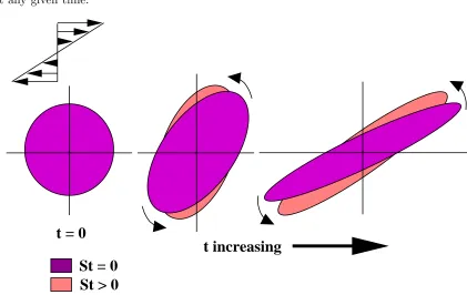
distorts iso-probability contours into ellipses, which stretch and align themselves with the flow as t → ∞. In the limit of long times, the inclination of the major axis of the ellipse with the flow direction is given by θ = (1/2) tan−1(3/t), and thus tends to zero as t → ∞. For finite St, not considering the O(St) corrections to the initial conditions, the effect of the off-diagonal diffusive term is to endow the probability ellipse with an ‘inertia’ which resists the tilting effect of the flow (see Fig 2.1), slowing it by O(St); indeed, for this case θ = (1/2) tan−1(3/t+ 3St/2t2), and is therefore greater than its inertialess value by O(St)
4For m=n = 0, it is easy to determine the complete expression for ∂/∂t
5 and to prove the absence of
fourth-order derivatives in ∂/∂t6, both of course acting on b(0i,)0(org). Thus, to O(St2), the equation for g
becomes
∂g ∂t2
+y∂g
∂x = 1 P e
∂2g ∂x2 +
∂2g ∂y2
− St
P e ∂2g ∂x∂y−
3St2
2P e
at any given time.
St > 0
St = 0
t = 0
[image:46.612.107.528.81.347.2]t increasing
Figure 2.1: Iso-probability contours in simple shear flow for St≥0.
In the limit of vanishing Brownian motion (P e → ∞), the inertial corrections vanish for any finite value of St, and (2.40) simplifies to
∂g ∂t2
+y ∂g ∂x = 0,
which has the general solutionF(x−yt2), leading to a number density that remains constant
flow (u = Gy, v =−Gx, G being the angular velocity) for finite St, the particle will follow a path that spirals outwards due to centrifugal forces in contrast to the purely tangential motion of the fluid elements. The case of simple shear flow of a suspension is similar since the hydrodynamic interactions between particles now cause the particle pathlines to become curved, and thereby deviate from the rectilinear pattern of the ambient field.
The solution to the corrected Smoluchowski equation (2.40) is of the form g = g0 +St g1, where g0 is the solution of the leading order Smoluchowski equation, and is
obtained from knowledge of the Green’s function of (2.40) and the initial condition at leading order. The Green’s function is (see Appendix A5) G(x, y, t|x0, y0, t0) from equation (A.61),
and satisfies G(x, y, t0|x0, y0, t0) = δ(x −x0)δ(y −y0). The O(St) correction g1 = gh1 +gp1,
wheregh
1 is the homogeneous solution satisfying the initial condition at O(St), andgp1 is the
particular solution given by5
gp1 =− 1 P e
t2 2
2 ∂2g
0
∂x2 +t2
∂2g 0
∂x∂y
. (2.42)
For the velocity distributions considered, we have from (2.41) (also see sections 2.4.1 and 2.4.2),
g0d(x,0) =δ(x)δ(y), g1d(x,0) = − 3
2P e[δ
00(x)δ(y) +δ(x)δ00(y)],
g0m(x,0) =δ(x)δ(y), g1m(x,0) = − 1
P e[δ
00(x)δ(y) +δ(x)δ00(y)],
where the superscriptsd and m, as before, indicate the initial conditions corresponding to a
delta function and a Maxwellian in velocity space, respectively. The solutions forg, toO(St), for the two cases are
gd(x, t2;St) =G0−
St P e " 3 2 (
∂2G0
∂x2 +
∂ ∂y +t2
∂ ∂x 2 G0 ) +
t22 2
∂2G0
∂x2 +t2
∂2G0
∂x∂y
#
,
=G0−
St P e
(4t22+ 3) 2
∂2G0
∂x2 + 4t2
∂2G0
∂x∂y + 3 2
∂2G0
∂y2
, (2.43)
gm(x, t2;St) =G0−
St P e
"(
∂2G0
∂x2 +
∂ ∂y+t2
∂ ∂x 2 G0 ) +
t22