LIQUID, SPIN LIQUID, AND MAGNETIC
PHASES
Thesis by
Tiamhock Tay
In Partial Fulfillment of the Requirements for the Degree of
Doctor of Philosophy
California Institute of Technology Pasadena, California
2011
c
2011
Acknowledgements
This dissertation would not be possible without the guidance of my thesis advisor, Lesik Motrunich, who has been very encouraging, patient, always willing to teach, and always finds time to discuss any issue I have whenever I knock on his office door. Despite being instrumental in directing much of the progress in our work, Lesik has always refused to take the credit and would always encourage me by highlighting my contributions. I also would like to thank Gil Refael for sharing his insights and views, which have helped to shape some of my perspective of physics. To my Caltech friends – Heywood Tam, Hsin-hua Lai, Wei Liang, Jing liu, Liyan, Zhaorui, Xiaowei, and many others whom I had the privilege to interact with – I wish to thank them for having enriched my experience here.
Abstract
Contents
Acknowledgements iv
Abstract v
1 Introduction 1
1.1 Overview of thesis . . . 1
1.2 Triangular antiferromagnet in magnetic field . . . 3
1.3 Exciton Bose Liquid . . . 6
1.4 Kagome antiferromagnet . . . 8
2 Preliminaries 11 2.1 Spin-wave analysis of the triangular Heisenberg model . . . 11
2.2 Parton-gauge perspective on the Exciton Bose Liquid . . . 15
2.3 Schwinger boson Spin liquid . . . 19
2.4 Quantum Monte Carlo Techniques . . . 22
2.4.1 Variational Monte Carlo . . . 22
2.4.2 Green’s Function Monte Carlo . . . 24
3 Heisenberg antiferromagnet on triangular lattice 29 3.1 Introduction . . . 29
3.2 Isotropic triangular antiferromagnet: 6×6 Study . . . 32
3.2.1 uud state atn = 1/3 . . . 32
3.2.2 Y state atn &1/3 . . . 33
3.2.3 Spiral state at n .1/2 . . . 35
3.2.4 V state atn .1/3 . . . 36
3.2.5 V state atn ≪1/3 . . . 37
3.2.6 Summary of trial energies on the isotropic lattice . . . 40
3.2.8 2-parton trial wave functions and alternative construction of
uud state atn = 1/3 . . . 41
3.3 Anisotropic triangular antiferromagnet . . . 44
3.3.1 Anisotropic Versions of Wave Functions . . . 45
3.3.2 n= 1/3 . . . 48
3.3.3 n= 1/6 . . . 50
3.3.4 Incommensurate V versus spiral study at low to intermediate boson densities . . . 51
3.3.5 Summary of Anisotropic Study . . . 54
3.4 Summary and discussion . . . 56
3.A Motivation for Vperm wave function forn .1/3, Eq. (3.11) . . . 57
3.B Correlation Functions of Permanent-type States . . . 58
4 Realization of Exciton Bose Liquid on a ring-exchange model 60 4.1 Introduction . . . 60
4.2 Variational study atρ= 1/2 . . . 62
4.2.1 Formal properties of the EBL wave function . . . 62
4.2.2 K1-K2 energetics study with one-parameter EBL wave function 66 4.3 Unbiased GFMC study at ρ= 1/2 . . . 68
4.3.1 Test of our GFMC setup . . . 70
4.3.2 GFMC study of theK1-K2 model at half-filling . . . 70
4.3.3 More detailed comparison with the EBL theory and interpreta-tions . . . 77
4.3.4 Interpretation of the failure of the VMC at ρ= 1/2 . . . 78
4.4 Study of the K1-K2 model for ρ <1/2 . . . 79
4.4.1 VMC results for 24×24 lattice . . . 80
4.4.2 GFMC results forL≤12 lattices . . . 81
4.5 Summary and discussion . . . 84
5 Failure of Gutzwiller wave function to capture gauge fluctuations 86 5.1 Introduction . . . 86
5.2 Effective actions for the EBL and Gutzwiller theories . . . 89
5.3 Trial wave functions . . . 92
5.3.1 General Jastrow wave function and harmonic approximation . 93 5.3.2 EBL wave function . . . 93
5.3.3 Gutzwiller wave function . . . 94
5.5 Summary and discussion . . . 101
6 Schwinger boson spin liquids on Kagome lattice 103 6.1 Introduction . . . 103
6.2 Schwinger-boson mean field ansatze . . . 104
6.3 Accessibility of Schwinger-boson spin liquid . . . 105
6.4 Variational Monte Carlo study . . . 106
6.5 Results . . . 109
6.6 Summary and discussion . . . 110
Chapter 1
Introduction
1.1
Overview of thesis
In this thesis, we study a pure ring-exchange model on the square lattice with the ob-jective of realizing the exciton Bose liquid (EBL) phase first proposed by Paramekanti, Balents and Fisher. The EBL is an unconventional quantum phase in which bosons do not condense and are not localized by interactions. With an unusual “Bose sur-face” in the energy spectrum analogous to the Fermi surface in a metal, the lines of gapless excitations in the Brillouin zone result in low temperature properties different from conventional bosonic phases. In earlier numerical studies, single-boson hopping was found to result in an instability to superfluid order, and pure ring exchanges on 1×1 plaquettes instead realize a (π, π) charge density wave (CDW). To suppress the superfluid and the CDW orders, we exclude single-boson hopping and introduce competing ring terms on 1×2 and 2×1 plaquettes. Our main interest here is whether this unconventional phase can be realized in a concrete Hamiltonian. We set up a Green’s Function Monte Carlo simulation which allows us to obtain a numerically exact phase diagram. We obtain a strong evidence that the EBL is realized for boson density less than 1/2. We find that the system is unstable to phase separation at low densities. This is not surprising since the bosons can gain energy from the ring exchanges only when they are sufficiently close to one another. At half-filling, we obtain theπ×π CDW order in the parameter regime close to the original 1×1 ring model, and the EBL phase when the 1×2 and 2×1 ring exchanges dominate. In the intermediate regime for the parameter, we obtain a Valence Bond Solid (VBS).
only while the other move vertically. By coupling the partons to the gauge field with opposite gauge charges, we show that the low energy effective theory of the parton-gauge system realizes the EBL theory. In this picture, the ring interaction between two bosons can be interpreted as an exchange of partons. The critical question that we attempt to address here is whether the widely used Gutzwiller projection for obtaining a variational wave function from slave particle wave functions is able to capture the spatial gauge fluctuations in a gauge theory. We compare an exact EBL wave function and a Gutzwiller wave function for hard-core bosons and find qualitative differences in the low energy properties such as the density structure factor and decay in the correlation at large distances, thus verifying our intuition that Gutzwiller wave functions might not accurately capture the true physics.
We also investigate magnetically ordered states and quantum liquids from a vari-ational perspective. Due to the lack of unbiased numerically exact tools in the study of frustrated systems, the well known sign problem presents a difficulty for quantum Monte Carlo. For this reason, we use the variational Monte Carlo (VMC) to identify candidate ground states among competing trial states in spin-1/2 Heisenberg antifer-romagnets on the triangular and kagome lattices, where a combination of geometrical frustration and small spin on the low-dimensional lattice leads to enhanced quantum fluctuations and interesting physics.
θ θ
(a)
θ1 θ2
(b) (c)
θ θ
[image:11.612.147.502.53.154.2](d) (e)
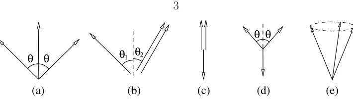
Figure 1.1: Spin orderings of the classical ground states, which we denote using (a) Ψ, (b)V, (c)uud, (d)Y, and (e)spiral. For each of these orderings, the three arrows represent the spin orientations on the three sublattices of the triangular lattice.
RVB states which consist of linear combinations of dimer covers. We find that the amplitude of the singlet bonds can be tuned from a quasi long-range decay to an exponential decay by varying the chemical potential in the mean-field Hamiltonian. The closing of the spinon energy gap at a critical value of the chemical potential results in condensation of spinons and consequently, producing a wave function with magnetic order. Thus, the range of the singlet bonds helps to provide an indication whether the variational ground state is spin-disordered or close to realizing a magnetic order. Using these RVB states constructed from the slave-particle approach, we compare the energies of the projected Schwinger boson wave functions against other competing variational states for the first- and second-nearest-neighbor J1-J2 Heisenberg model. We find that the projected Schwinger boson wave function is a viable candidate for J2 >0.08J1.
The remainder of this chapter provides a more detailed introduction to each of the studies described above, while the following chapter contains simple theoretical treatments of the models which bridge the gap to the material in later chapters. Chapters 3 to 6 are a collection of published papers[1, 2, 3, 4, 5] co-authored with my thesis advisor, Olexei I. Motrunich. It is a pleasure to acknowledge his important, extensive contributions which have unveiled the interesting physics in the study of these strongly correlated systems.
1.2
Triangular antiferromagnet in magnetic field
orientations as depicted in Fig. 1.1. The spiral and Y orderings have equal energies at low fields, while V, Ψ, and spiral have equal energies at high fields. At 1/3 of the saturation field, the Y and V orderings reduce to the uud, which also has the same energy as the spiral and Ψ orderings.
The degeneracies in the classical ground states are lifted by thermal fluctuations at finite temperatures. In a classical Monte Carlo study by Kawamura et al.[6], the coplanar Y and V orderings are found to be selected at low and high magnetic fields respectively, while the collinearuud ordering is increasingly stabilized with tempera-ture at intermediate fields. For the isotropic quantum model at zero temperatempera-ture, a semi-classical analysis by Chubukov et al. shows that quantum fluctuations also se-lect the same coplanar and collinear orderings[7]. Theuudhas been predicted to give rise to a 1/3-magnetization plateau (see Fig. 3.5 on page 41) but was first observed much later in a high field magnetization study by Ono et al. on the nearly isotropic Cs2CuBr4[8]. A more recent experiment by Fortune et al. further reveals a cascade of quantum phase transitions in magnetocaloric and magnetic-torque measurements made on the same chemical compound[9].
A similar attempt to identify the newly discovered phases using the semi-classical analysis would immediately run into difficulty. In fact, an incommensurate generaliza-tion of the spiral phase becomes the unique classical ground state of the anisotropic model at all fields, hence spin-wave expansions about other classical orderings such as the uud are not allowed for finite anisotropy. This issue was overcome by
Al-icea et al.[10] by extending the large-S expansion to an interacting spin-wave theory
controlled by large spin as well as small spatial anisotropy. Their theoretical results show that strong quantum fluctuations again select the uud state at intermediate fields as well as the coplanar orderings in its vicinity. The uud plateau extends con-siderably into the anisotropic region, and they also obtain incommensurate coplanar and distorted spiral phases for larger anisotropy.
for an anisotropy relevant to Cs2CuCl4 and found that the incommensurate spiral dominates near the saturation field, but undergoes phase transition at a slightly lower field to a commensurate non-coplanar ordering[12].
From the decoupled-chain limit, Starykh et al. argues that the interchain cou-pling is a relevant perturbation and can induce various boson CDW phases or a spiral phase[13]. The former happens for small and intermediate fields, while the latter is expected near the saturation field. In zero magnetic field, their study predicted a collinear antiferromagnetic order while variational studies suggest that the non-coplanar spiral phase is stable for small lattice anisotropy[14], and the intermediate anisotropic region may contain one or two spin liquid phases[15, 16]. This is sup-ported by an ED/DMRG study which found signatures of spin liquid forJ′/J <0.78
from numerical measurements of spin structure factor, excitation energy gap, and spin correlation[17].
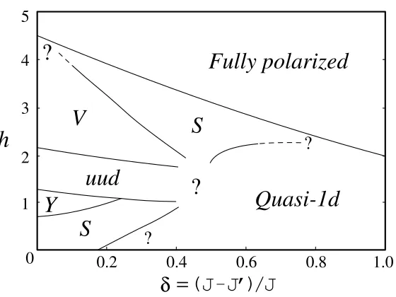
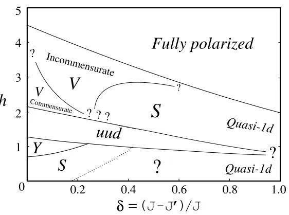
In Chapter 3, we investigate the anisotropic Heisenberg model in magnetic field by studying the equivalent hard-core boson model using the variational approach. Here, we provide a summary of our results in reference to a schematic phase diagram shown in Fig. 3.10 on page 55. Starting from the 1/3-magnetization for the isotropic regime, we construct an accurate Mott insulator wave function which features a short range correlation between every pair of sites. This wave function naturally generalizes to the nearby commensurate coplanarY and V states which are realized as supersolid states in the hard-core boson picture. Interestingly, the Y wave function has a short range correlation when at least one site resides on the “down” sublattice (see Fig. 1.1d). This contrasts with the long range correlation when both sites belong to the remaining sublattices. For the V phase, we construct a supersolid wave function having long range correlations between all sites on the lattice. Our accurate wave functions allow us to obtain upper and lower critical fields of the plateau which agree quantitatively with other studies. For magnetic fields close to zero, we find that Huse and Elser’s spiral wave function[14] performs better than the Y state.
a consequence of finite-size effects, thus suggesting that other numerical techniques such as the Density Matrix Renormalization Group (DMRG) would be necessary for unveiling the physics in the quasi one-dimensional regime.
1.3
Exciton Bose Liquid
The search for exotic quantum phases has gained a very wide audience in recent years. A number of years ago, Paramekanti et al.[18] proposed an interesting critical bosonic phase which shares many characteristics normally associated with electrons in a metal. Starting with a bosonic ring exchange model on the square lattice, where two bosons hop simultaneously on opposite corners of an elementary square plaquette to the other two corners, they derived a low energy effective Lagrangian in terms of the boson phase variable and its dual vortex phase variable. The effective theory demonstrates a remarkable similarity to the bosonized action for a one-dimensional Luttinger liquid, and can be traced back to the “dimensional reduction” of the system which results from the conservation of boson numbers along each row and each column of the square lattice. The energy spectrum of the system features lines of gapless excitations (see Fig. 1.2) that are responsible for various properties of the system such as a power-law decay in the correlations and a specific heat varying as T log(1/T). A striking parallel to electrons in a metal is pointed out by Sachdev[19], where the Fermi surface separates occupied electron states from the vacant states. Here, the zero energy lines in Brillouin zone can be analogously termed the “Bose surface” since low energy excitations of the system occur near this surface, and Bose-condensation does not occur in the system.
Figure 1.2: The EBL phase is characterized by a “Bose surface”, that is, the lines of gapless excitations in the Brillouin zone (i.e.,kx = 0 or ky = 0) which are responsible for the unusual low temperature properties.
The striking proposal of Paramekanti et al. stimulated a number of works which seek to establish the stability of the EBL phase in hard-core boson models with ring exchange interactions on the square lattice[20, 21, 22, 23]. However, these studies found that the EBL is not realized in these models. Instead, such ring interactions favor a (π, π) charge density wave (CDW) in the filled case, while away from half-filling they induce strong tendencies to phase separation. With a goal of realizing the novel EBL phase, we attempt to suppress the CDW order by adding competing ring exchanges to the system. We consider in Chapter 4 a specific hard-core boson model with competing ring-only exchanges on a square lattice, where aK1 term acts on 1×1 plaquettes and a K2 term acts on 1×2 and 2×1 plaquettes. We construct Jastrow-type variational wave functions for the EBL and study their formal properties using Variational Monte Carlo. The optimized trial wave functions are then used as starting points for a projective Quantum Monte Carlo study. Using Green’s Function Monte Carlo, we obtain an unbiased phase diagram (cf. Fig. 4.14 on page 83) which at half-filling reveals CDW for small K2, valence bond solid for intermediate K2, and possibly for large K2 the EBL phase. Away from half-filling, we argue that the EBL phase is present for intermediateK2 and remains stable for a range of densities below 1/2 before phase separation occurs at lower densities.
show that the Gutzwiller projection indeed leads to a state with subtle differences in the long-wavelength properties, thus suggesting that Gutzwiller wave functions may generally fail to capture long-wavelength physics.
1.4
Kagome antiferromagnet
In recent years, interest in the spin-1/2 Heisenberg antiferromagnetic model on the kagome lattice has been re-ignited by exact diagonalization (ED) and Density Matrix Renormalization Group (DMRG) studies which provide stronger evidence that the ground state of the system realizes a spin liquid[24, 25, 26]. At the classical level, geometrical frustration is known to result in a macroscopically large number of degen-erate ground states. This is easily seen by noting that any classical spin configuration having its spins oriented at 120◦ apart on every elementary triangular plaquette is
a ground state of the system. Thus, listing down these states amounts to assigning one out of three possible spin orientations (denoted A, B, and C) to every site such that no two nearest neighbors point in the same direction. As an illustration, Fig. 1.3 shows three out of 504 possibilities for a 36-site cluster with periodic boundary condi-tion. In addition to this huge degeneracy among coplanar states, the plane formed by any closed loop containing only two spin directions (e.g., A–B–A–B–A–B–A around an hexagon) can be rotated about the third direction (i.e., C) without incurring an energy penalty. This huge number of continuously degenerate ground states therefore cast doubts on the validity of a spin-wave expansion of the quantum model about a specific classical ordering, and instead raises the prospect of the system realizing a spin-disordered ground state.
Numerical evidence from ED and DMRG studies indicates that the Heisenberg antiferromagnet on the kagome lattice does not have any magnetic or valence bond ordering[27, 28, 25, 29]. These studies found short ranged spin-spin correlations and a finite spin gap estimated at J/20, where J is the nearest-neighbor coupling constant[28, 25, 26]. Interestingly, a large number of singlet excitations are observed in the spin gap[25]. On the experimental side, the lack of a magnetic order persists down to 50mK in the material Herbertsmithite which contains weakly coupled layers of spin-1/2 kagome antiferromagnets[30, 31, 32, 33]. Thus, there is a convergence of views over the years that the isotropic spin-1/2 Heisenberg antiferromagnet with only nearest-neighbor exchange indeed realizes a spin liquid.
A A A A A A A A A A A A B B B B B B B B
B B B
B C C C C C C C C C C C C
(a)q=0
C A A B B C C A A C B B A B C B A C B C
B C A
A A B C B C B A A B C A C
(b) √3×√3
C A B A B C C B B C A A B A C A B C B C
A C A
B B A C A C A B A B C B C (c)
Figure 1.3: Illustration of three possible spin orderings out of a total of 504 for a periodic 36-site cluster, where A, B and C denotes three coplanar vectors with 120◦
between them. These states have identical energy for the classical model, but the degeneracy may be lifted by thermal or quantum fluctuations.
bond crystal with a 36-site unit cell as the ground state, contractor renormalization (CORE)[37, 38], and multi-scale entanglement renormalization ansatz (MERA)[39].
Slave-particle approaches have also been used to explore the possible nature of the spin liquid ground state. An early study by Sachdev using Sp(N) Schwinger bosons in the large-N limit found the √3×√3 magnetically ordered ground state[40] for spinS >0.26, depicted in Fig. 1.3(b). Analysis of the gauge field fluctuations showed that the spinons remain deconfined for S < 0.26, while they condense for larger spin and result in the magnetic ordering. Attempts to extend the spin liquid regime to the physical spin S = 1/2 would fail to address the continuum of singlet excitations found in the spin gap by ED studies[25], since the Schwinger boson spinon spectrum is gapped. A different approach by Hastings uses slave fermions to construct a long range Resonating Valence Bond (RVB) state with a Dirac structure in the spinon spectrum[41]. Hastings’ state, also known as the Dirac spin liquid, is appealing since it contains low energy gauge excitations. A subsequent Gutzwiller projection on the mean-field Dirac spin liquid wave function by Ran et al. obtained a variational energy which lies close to the ED ground state energy[42, 27].
basis has been implemented for a projected Schwinger boson wave function on the triangular lattice[43]. The latter suffers from a less severe form of sign problem and such calculations are similarly restricted to small system sizes. For our study in Chapter 6, we extend the nearest-neighbor model to theJ1-J2 Heisenberg model with antiferromagneticJ2 coupling[44], and investigate the energetics of various wave func-tions. We find that Sachdev’s Q1 =Q2 Schwinger boson ansatz is a viable candidate for J2 &0.08J1 due to a stronger second-neighbor antiferromagnetic spin correlation compared to the Dirac spin liquid. For J2 . −0.04J1, Sachdev’s Q1 = −Q2 ansatz performs well due to its ferromagnetic second-neighbor correlations. Thus, our study shows that the Schwinger boson wave functions may still be relevant despite being eclipsed by the Dirac spin liquid wave function in recent years.
Chapter 2
Preliminaries
In this chapter, we discuss some of the models in this thesis using simpler or less accurate theoretical treatments for some special cases, with the purpose of bridging the transitional gap to the material presented in later chapters. In Sec. 2.1, we analyze the isotropic Heisenberg antiferromagnet in magnetic field using a spin-wave approach and discuss how this approach breaks down for the anisotropic lattice. Our variational Monte Carlo treatment in the next chapter allows us to compare competing phases identified by other theoretical approaches. This is achieved by constructing accurate wave functions which help to determine candidate quantum phases. In Sec. 2.2, we provide a parton-gauge perspective to the Exciton Bose Liquid phase whose interesting properties had motivated our search for a realizable concrete model in Chapter 4. In Sec. 2.3, we analyze the nearest-neighbor Heisenberg antiferromagnet on the kagome lattice using a mean-field Schwinger boson slave-particle treatment, while leaving the full analysis for the extension to the second-neighbor Heisenberg model to Chapter 6. Finally, in Sec. 2.4, we discuss the Monte Carlo implementations used in this thesis.
2.1
Spin-wave analysis of the triangular
Heisen-berg model
The nearest-neighbor antiferromagnetic Heisenberg spin model on an isotropic trian-gular lattice in magnetic field is given by the following Hamiltonian:
H =JX
hi,ji
Si ·Sj−~h·
X
i
whereJ is the coupling strength between spins on nearest-neighbor sitesiandj of the triangular lattice. Due to geometrical frustration on the lattice, it is not possible to saturate the lower bound in the interaction energy for every pair of nearest-neighbors. This results in degenerate ground states in the corresponding classical model at all magnetic fields. To see this, we note that the classical Hamiltonian is minimized when the spin configuration has a three-sublattice structure
Ecl/site = JS2(ˆnzA·nˆzB+ ˆnzB·ˆnzC + ˆnzC ·nˆzA)− 1
3~h·S(ˆn z
A+ ˆnzB+ ˆnzC), (2.2)
= 3 2JS
2
− 181 h2/J +1 2JS
2 nˆz
A+ ˆnzB+ ˆnzC − ~h 3JS
!2
, (2.3)
where ˆnz
A, ˆnzB and ˆnzC are unit vectors along the directions of the spin orderings on sublattices A, B and C. The ground state spin configurations satisfy
~h = 3JS(ˆnzA+ ˆnzB+ ˆnzC), (2.4)
and the only possible orderings are shown in Fig. 1.1, where we denote them by (a) Ψ, (b) V, (c) uud, (d) Y, and (e) spiral. The saturation field h= 4.5J for the spin-1/2 classical model follows from Eq. (2.4), and this value also holds for the quantum model. Forh <1.5J, thespiraland Y states are degenerate ground states, while for 1.5< h/J <4.5, the states V, Ψ, andspiral are degenerate. At h = 1.5J, all of the states shown in Fig. 1.1 have the same energy. In addition to these degeneracies, the energy is invariant under a rotation about the magnetic field.
In the presence of quantum fluctuations, some or all of the degeneracies existing in the classical model may be lifted. In the following, we apply the Holstein-Primakoff transformation:
S+ = p2S−a†a a≈√2Sa, (2.5)
S− = a†p2S−a†a≈√2Sa†, (2.6)
where a† is a bosonic creation operator, and obtain a spin-wave Hamiltonian
(HSW−Ecl)/JS = 1 2
X
k
νk(ˆea·eˆb a−kbk+ ˆeb·eˆc b−kck+ ˆec·eˆa c−kak)
+ 1 2
X
k
νk
ˆ
e∗a·ebˆ a†kbk+ ˆe∗b ·ecˆ b
†
kck+ ˆe∗c ·eaˆ c
†
kak
+ H.c.+ 3X
k
(a†kak+b†kbk+c†kck), (2.8)
whereνk=Pµeik·µˆand ˆeα= ˆnxα−iˆnyα. Here,a,b, andcare the annihilation operators on the respective sublattices, {µˆ} are three unit vectors on the lattice which make an angle 120◦ with one another, and ˆnj
α specifies the orientation of the local j-axis on sublatticeα. For non-collinear spin orderings, Eq. (2.4) is used to eliminate terms that are linear in the bosonic operators.
The spin-wave Hamiltonian can be diagonalized using Bogoliubov’s transforma-tion. For a general Hamiltonian that is quadratic in the bosonic operators, we may express it as follows:
H = α~†D~α, (2.9)
~
α = (γ1,· · · , γn, γn+1† ,· · · , γ2n† )T, (2.10) [αi, αj] = ηij ≡diag(1,· · · ,1,−1,· · · ,−1), (2.11)
where {γi} are 2n independent bosonic annihilation operators. If a canonical trans-formation α~ = U ~β results in a diagonal matrix Λ = U†DU, then U and Λ must
satisfy
U†ηU = η, (2.12)
(ηD)U = U(ηΛ). (2.13)
Since D is positive definite, the eigenvalues of the system are simply given by the absolute values of the corresponding eigenvalues ofηD.
-0.06 -0.04 -0.02 0.00
0.0 1.5 3.0 4.5
(E - E
cl
) / J
h / J
spiral Y uud V
[image:22.612.152.494.79.323.2]Ψ
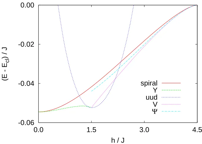
Figure 2.1: Comparison of the spin-wave energies (per bond) for each of the spin orderings listed in Fig. 1.1. The constant magnetization of the uud state leads to a 1/3-magnetization plateau for 1.4< h/J <2.17 on an isotropic lattice (see Fig. 3.5).
the high field regime extending up to saturation is dominated by the V state. Inter-estingly, the uud state is stable over the range 1.39< h/J < 2.17 despite a smooth interpolation between the classicalY and V configurations through the uud ordering as h approaches 1.5J. This results in a 1/3-magnetization plateau on the triangu-lar lattice (see Fig. 3.5 on page 41) and was observed in Cs2CuBr4[8]. In principle, renormalizations of the spin orientations may result from quantum fluctuations[7] and would lead to shifts in the upper and lower critical fields of the uud phase, but we have not taken this into consideration here. In contrast to the gapless spectra for the non-collinear spin orderings, we observe a finite gap in the uud spectrum which agrees with the absence of Goldstone modes since continuous symmetry has not been broken.
repeated for the anisotropic lattice would show that thespiral is the unique classical ground state at all magnetic fields. The semi-classical spin-wave treatment therefore runs into a difficulty since Cs2CuBr4 has been found to realize the 1/3-magnetization plateau despite having an anisotropy estimated to be J′/J ∼ 0.7. Our approach to
the problem is to study an equivalent hard-core boson model using variational Monte Carlo. In the bosonic picture, the spin orderings have interesting interpretations – namely, superfluid, supersolids and a Mott insulator. We study the model on the anisotropic lattice and obtain a very rich phase diagram (see Fig. 3.10). Possible im-plications to the triangular antiferromagnets Cs2CuBr4 and Cs2CuCl4 are discussed there.
2.2
Parton-gauge perspective on the Exciton Bose
Liquid
In this section, we provide a parton-gauge perspective on the EBL phase. The EBL phase is defined by a fixed point Lagrangian[18]
L0 =
X
r
i
π∂τϕ(r)∆xyϑ(R) +
Z
k
K(k)
2 |(∆xyϕ)k|
2+U(k)
2π2 |(∆xyϑ)k| 2
, (2.14)
where ϕ is the phase of a bosonic field andϑ is related to the boson density through n−n¯ = π1∆xyϑ. The “EBL parameters” K(k) and U(k) are functions of k which respect the square lattice symmetries[18]. Long-wavelength properties such as various power-law exponents depend only on the functionK(0, ky)/U(0, ky). Notice the strong similarity between this Lagrangian and the bosonized action for Luttinger liquid. An effective “dimensional reduction” noted by some authors[18, 45, 46, 47, 48, 49] is suggestive of a decomposition of each boson into two partons with one-dimensional (1D) character, interacting strongly via a gauge field. Below, we show that the gauge fluctuation effects can be treated accurately and lead to the same EBL description. We will also see how the familiar 1D Bosonization techniques[50, 51] allow us to quickly obtain physical observables and important residual interactions in the EBL theory. We emphasize, however, that the EBL phase is qualitatively different from sliding or crossed-sliding Luttinger liquids[52, 53, 54, 55]—for example, it has specific heat C ∼T ln(1/T), cf. Ref. [18].
parton-gauge system, we consider the following Lagrangian:
L[ϕ1, θ1, ϕ2, θ2, ax, ay] = X
r
κ
2(∇xay− ∇yax)
2 (2.15)
+ X
r
hJ
2(∇xϕ1−ax) 2+u
2
∇xθ1
π
2
+ i
π∂τϕ1∇xθ1
i
+ X
r
hJ
2(∇yϕ2+ay) 2+u
2
∇yθ2
π
2
+ i
π∂τϕ2∇yθ2
i
.
The phase and dual variables ϕ1(x, y) and θ1(X, y) describe a harmonic fluid[50, 51] of partons moving on a horizontally oriented chain located at a vertical coordinatey, while variablesϕ2(x, y) andθ2(x, Y) describe a harmonic fluid of partons moving on a vertically oriented chain at a horizontal coordinatex. Note thatϕ1(x, y) andϕ2(x, y) reside on the sites of the original lattice, whileθ1(X, y) resides on the horizontal links and θ2(x, Y) on the vertical links as illustrated in Fig. 2.2. The coupling parameters J and u represents parton hopping and on-site repulsion, respectively. Note that we assume a stable phase where (ax, ay) can be treated as a non-compact gauge field with a large “stiffness” parameter κ. The parton densities are given by
n1(x, y) = 1
π∇xθ1, (2.16)
n2(x, y) = 1
π∇yθ2, (2.17)
and we now introduce the following constraint to realize the microscopic boson in the EBL phase using a 2-parton composite:
∇xθ1 =∇yθ2 . (2.18)
At this stage, we can integrate out the fields ϕ1 andϕ2 and obtain the Lagrangian density
l[θ1, θ2, ax, ay] = u
2π2
(∇xθ1)2+ (∇yθ2)2
+ 1 2π2J
(∂τθ1)2+ (∂τθ2)2
+ i
π(ax∂τθ1−ay∂τθ2) + κ
2(∇xay − ∇yax)
(X,Y)
(X,y)
(X,Y−1) (x,Y)
(x,y)
(x,Y−1) (X−1,Y)
(X−1,y)
[image:25.612.235.413.52.254.2](X−1,Y−1)
Figure 2.2: The parton phase fieldsϕ1(x, y), ϕ2(x, y) reside on the sites of the original square lattice (black circles); the 1D dual field θ1(X, y) resides on the horizontal links and θ2(x, Y) on the vertical links (white boxes). The dual EBL theory field ϑ(X, Y) resides on the plaquettes of the original lattice, or equivalently on the sites of the dual lattice (stars).
We then solve the constraint Eq. (2.18) via
θ1(X, y) =∇yϑ ≡ϑ(X, Y)−ϑ(X, Y −1), (2.20)
θ2(x, Y) =∇xϑ ≡ϑ(X, Y)−ϑ(X−1, Y) , (2.21)
cf. Fig. 2.2. Integrating out the field a, we finally obtain Lagrangian density
l[ϑ] = u
π2(∇ 2
xyϑ)2+ 1
2π2J(∂τ∇ϑ)
2+ 1
2π2κ(∂τϑ)
2. (2.22)
This is essentially the EBL theory written in the dual variables ϑ [after integrating out the ϕ variables from Eq. (2.14)], with U(k) = 2u and 1/K(k) = 4[sin2(kx/2) + sin2(k
y/2)]/J+ 1/κ. Note that one may be tempted to drop the (∂τ∇ϑ)2/J term as it contains more derivatives than the (∂τϑ)2/κterm. However, the long-distance EBL properties such as power-law exponents are determined by the full function K(0, ky) which does depend on J if we want to be accurate in the simple model Eq. (2.15) that we took. If we include from the start general interactions among the partons and general Maxwell terms for the gauge field, we obtain the general Gaussian EBL theory with k-dependent K(k) and U(k).
and bond energy are given by
δn1(r) = ∇xθ1
π +Acos [2θ1+ 2πn(x¯ −1/2)] , (2.23) δBr,r+ˆx = A′cos [2θ1+ 2πnx]¯ . (2.24)
Hereθ1 already means the long-wavelength component and the precise location where it is evaluated along the chain is unimportant. In terms of the original variables of the EBL theory [replacing θ1 by Eq. (2.20)], we obtain
n(r) = ¯n+δn0+Acos[2∇yϑ+ 2π¯n(x−1/2)]
+ Acos[2∇xϑ+ 2π¯n(y−1/2)] , (2.25)
δBr,r+ˆx = A′cos[2∇yϑ+ 2π¯nx] . (2.26) We can also express inter-chain density-density interactions
Vjn1(r)n1(r+jyˆ) ∼ Vjcos [2θ1(r) + 2θ1(r+jyˆ) + 4π¯nx−2π¯n]
+ Vjcos [2θ1(r)−2θ1(r+jyˆ)], (2.27)
where we have only retained cosine terms. Written in terms of the ϑ fields, the first line is non-oscillatory only at half-filling and corresponds to the Umklapp interaction, while the second line is the non-Umklapp interaction.
Let us remark about the effects of compactness of the microscopic gauge field. As is known from the 1D folklore, allowing cosines of the dual fields in the action effectively allows vortices in the microscopic phase variables and provides a faithful treatment of the compactness of the phase variables. In this respect one may wonder about the status of our theory once we allow the described cosine terms in theθ1 and θ2 variables. It turns out that it is not complete yet, but becomes so after we allow terms like
Lv =−
∞
X
q=1
vqcos[q(2ϑ+ 2π¯nXY)], (2.28)
2.3
Schwinger boson Spin liquid
The Schwinger boson representation[56] of a spin S is given by
S= 1 2
X
σ,σ′
b†σσσσ′bσ′, (2.29) where{bσ, σ=↑,↓}are bosonic operators andσ are the Pauli matrices. The physical Hilbert space lies in the sector with P
σnσ = 2S. A standard recipe for constructing a spin liquid often begins from a schematic Heisenberg Hamiltonian and follows by a mean-field decoupling which leads to a solvable model. In terms of Schwinger bosons, the spin coupling between sites i and j may be written as
Si·Sj = : Bij†Bij :− A
†
ijAij, (2.30)
Aij = 1 2
X
σ,σ′
ǫσσ′biσbjσ′, (2.31)
Bij = 1 2
X
σ
b†iσbjσ, (2.32)
where : : denotes normal ordering. The decoupling leads to the mean-field Hamilto-nian
Hm.f. = 1 2
X
i,j
¯
Bij∗Bij + ¯BijBij† − |Bij¯ i|2 (2.33)
− 1
2
X
i,j
¯
A∗ijAij + ¯AijA†ij− |Aij¯ |2−µX i,σ
b†iσbiσ, where the chemical potential µis tuned to fulfill the conditionP
σhniσi= 2S at each lattice site. The collection of parameters {A¯ij} and {B¯ij} is treated as an ansatz which determines the type of spin liquid realized by the ground state.
a
b
c
Figure 2.3: The Schwinger boson ansatze from Ref. [40], where Aij = 1 if an arrow points from site ito a nearest-neighbor sitej,−1 for the opposite direction, and zero for all further neighbors. The shaded region shows a unit cell of the ansatz, and a, b and c label the three bosonic operators in each unit cell.
can be evaluated as follows:
hSi·Sji = hSii · hSji+ 1 2
X
α,β
hb†iαbjαihbiβb†jβi (2.34) + 1
4
X
α,β,σ
hb†iαb†jβ +σbiβ† b†jαihbiβbjα+σbiαbjβi
− 1
8
X
α,β,σ
hb†iαb†jβ +σb†iβb†jαihbiαbjβ+σbiβbjαi
− 1
8
X
σ
hb†i↑bj↑+σb†i↓bj↓ihbi↑b†j↑+σbi↓b†j↓i
= 3
2 |hBiji| 2
− |hAiji|2
. (2.35)
Equation (2.35) suggests that an energy cost is incurred for ansatze with ¯Bij 6= 0 when considering spin liquids on antiferromagnetic models. In Ref. [57], Wanget al. classi-fied all possibleZ2 symmetric spin liquids withA-only ansatze on the kagome lattice allowed by the Projective Symmetry Group analysis and showed that there are only four distinct classes for nearest-neighbor Aij. Below, we study one of the ansatze shown in Fig. 2.3 (first found by Sachdev[40]), which we denote by “q=0 ansatz.”
written in momentum space as follows:
H = X
k
Ψ†k
−µ iDk
−iDk −µ
Ψk+ 3µ
, (2.36)
Dk =
i 2
0 1 +e−ik·eˆ1 −e−ik·ˆe1 −eik·eˆ3
−1−eik·ˆe1 0 1 +eik·eˆ3
eik·eˆ1 +e−ik·eˆ3 −1−e−ik·eˆ3 0
, (2.37) ˆ
e1 = ˆx, eˆ2 = (ˆx+
√
3ˆy)/2, eˆ3 = (−xˆ+
√
3ˆy)/2, (2.38)
ΨTk = (ak↑, bk↑, ck↑, a†−k↓, b † −k↓, c
†
−k↓), (2.39)
where a, b and c are the three bosonic annihilation operators in each unit cell of the kagome lattice (see Fig. 2.3). The Hamiltonian can be simplified further by applying a 3×3 unitary transformation Mk onDk which gives
H = X
k,γ=a,b,c ˜ γk↑
˜ γ−†k↓
†
−µ iλk˜γ
−iλk˜γ −µ
˜ γk↑
˜ γ−†k↓
+µ
, (2.40)
˜ γk↑ =
X
α=a,b,c
(Mk)γα˜ αk↑, ˜γ−†k↓ =
X
α=a,b,c
(Mk)˜γαα−†k↓ , (2.41)
Λk = diag(λk˜γ) = MkDkMk† . (2.42)
It is now straightforward to diagonalize the Hamiltonian using a 2×2 Bogoliubov’s transformation and we obtain the following excitation spectrum:
ǫ(1)k =|µ|, ǫ(2)k =ǫ(3)k =pµ2−[3 + cos(k·ˆe
1) + cos(k·eˆ2) + cos(k·eˆ3)]/2. (2.43) The spinon spectrum is gapped forµ <−√3 and the q=0ansatz realizes a spin liquid wave function. As µ → −√3, the energy gap vanishes, causing the spinons to condense and resulting in a magnetically ordered state. By requiring that the expectation of the total boson density at each lattice is equal to 2S, we obtain
S = 1 3N
X
k
−1 + |µ| ǫ(2)k
!
≤0.25. (2.44)
value of S that separates the magnetically ordered phase for large spins from the spin-disordered phase for small spins. In Chapter 6, we improve upon the mean-field treatment by applying a Gutzwiller projection to enforce the stricter constraint
P
σnσ = 2S at each site. We study the energetics of the projected Schwinger boson wave functions in the spin-1/2 Heisenberg antiferromagnetic model with first- and second-neighbor couplings.
2.4
Quantum Monte Carlo Techniques
Quantum Monte Carlo (QMC) is a class of algorithms widely used to simulate many-body systems in physics. It allows us to study problems where analytically exact so-lutions or well-controlled approximations are not available. For unfrustrated strongly correlated models in two dimensions or higher, QMC is often the method of choice for obtaining unbiased information on the ground state or finite temperature properties and is therefore an invaluable tool. The essential ingredient of QMC algorithms is the stochastic approach of sampling important configurations in systems with large number of degrees of freedom.
Different flavors of QMC algorithms exist, for example, variational Monte Carlo (VMC), Diffusion Monte Carlo (DMC), Green’s Function Monte Carlo (GFMC), Path Integral Monte Carlo (PIMC), and Stochastic Series Expansion (SSE). In this thesis, we make extensive use of the VMC to investigate the ground state properties of a number of quantum lattice models. In the absence of frustration, where QMC does not suffer from the well-known sign problem, we set up a GFMC simulation which provides exciting evidence that a concrete realization of the exotic Bose Liquid phase may be possible in a hard-core boson model with ring-exchange interaction. In the remainder of this section, we review the VMC and GFMC techniques employed in this thesis.
2.4.1
Variational Monte Carlo
The variational Monte Carlo (VMC) approach relies on the variational principle, which states that the average energy ET of any trial wave function ΨT provides an upper bound to the exact ground state energy E0 of a system
E0 ≤ET = hΨT|H|ΨTi
and this forms the basis for the variational approach. By itself, VMC does not provide an exact solution of the problem but it instead allows one to identify a candidate ground state among competing wave functions. This is very useful in many problems where other unbiased QMC techniques fail due to the sign problem. In addition, it is often possible to implement contraints such as hard-core repulsion in wave functions where approximate treatments are rather crude. Thus, the VMC allows us to obtain reliable upper bounds using trial wave functions that lie in the physical Hilbert space. We apply the VMC technique to study the energetics of a variety of quantum phases ranging from insulator to magnetic orderings, spin liquids, and bose liquids. To assess the accuracy of a trial state, it is often useful to determine where the trial energy lies in relation to the exact diagonalization spectrum:
|ΨTi = X
i
ai|Eii, X i
|ai|2 = 1, (2.46) ET −E0
E1−E0 =
P
i|ai|2(Ei−E0) E1 −E0 ≥
X
i>0
|ai|2. (2.47)
Equation (2.47) shows that it is necessary for the trial energy of a variational wave function to be close to the ground state energy compared to the excitation gap in order to achieve a good overlap with the true ground state. However, it is important to note that the accuracy of other measurements such as correlation functions may not be satisfactory since variational energies are mainly sensitive to the local energetics[58]. The expectation value of an operatorO can be computed stochastically for a given trial state |ΨTias follows:
hOi=
P
xhΨT|O|xihx|ΨTi
P
xhΨT|xihx|ΨTi
=X
x
pxOx, (2.48)
px = PhΨT|xihx|ΨTi
x′hΨT|x′ihx′|ΨTi
, Ox = h
ΨT|O|xi
hΨT|xi , (2.49)
where |xi is a basis vector in the Hilbert space. The probability distribution {px} can be statistically sampled by generating a markov chain{xτ} using the metropolis algorithm, where an arbitrary configuration is selected at a time step τ and accepted with probability min(1, |hxτ|ΨTi|2
|hxτ−1|ΨTi|2). The expectation value of the operator becomes
hOi= 1 M
M
X
τ=1
This simple formulation allows us to study a large number of problems in quantum many-body systems.
2.4.2
Green’s Function Monte Carlo
The Green’s function Monte Carlo (GFMC) is a projector method used for studying the ground state properties of many-body quantum systems. Starting from an initial trial wave function with a sufficiently good overlap with the ground state of a system, a projection operator G is applied repeatedly to the trial wave function to filter out the excited states:
|ψgi= lim n→∞G
n
|ψTi. (2.51)
This iterative procedure is also known as the power method which singles out the eigenvector of G with the largest eigenvalue as n → ∞. Possible choices of the operator G include exp(−Hδτ) and 1−(H−Er)δτ, whereEr and δτ are chosen to ensure that the desired state is projected out. As with other Quantum Monte Carlo techniques, the GFMC can be used only if there is no sign problem, i.e., the matrix elements of Gare all positive in a known basis.
We now review Hetherington’s GFMC scheme[59] for calculating the expectation of the energy:
hHni = hΨT|HG n|φi
hΨT|Gn|φi , (2.52)
=
P
xExhΨT|xihx|Gn|φi
P
xhΨT|xihx|Gn|φi
, (2.53)
where |φi is a starting wave function for the projection and Ex is the “local energy” defined in Eq. (2.49). In the limit n→ ∞, hHni converges to the exact ground state energy. Defining
Gxy =hx|G|yi, φ(x) =hx|φi, (2.54)
and
˜
Gxy =hΨT|xiGxy/hΨT|yi, (2.55)
the energy becomes
hHni=
P
{xi}Exn ˜
Gxnxn−1· · ·Gx˜ 1x0ΨT(x0)φ(x0) P
{xi}Gx˜ nxn−1· · ·Gx˜ 1x0ΨT(x0)φ(x0)
To see how Eq. (2.56) can be evaluated stochastically, note that the non-negative matrix ˜G can be decomposed into the product of a diagonal matrix and a stochastic matrix ˜Kxy = ˜Gxy/by with by =P
xGxy. Equation (2.56) now becomes˜
hHni=
P
{xi}ExnKx˜ nxn−1bxn−1· · ·bx0P(xn−1,· · ·, x0) P
{xi}bxn−1· · ·bx0P(xn−1,· · · , x0)
, (2.57)
where P(xn−1,· · · , x0) = ˜Kxn−1xn−2· · ·Kx˜ 1x0ΨT(x0)φ(x0) may be interpreted as the
probability distribution for sampling the path {xn−1,· · · , x0}, and ˜Kxnxn−1 is the
probability for sampling the next configuration, xn. In a Monte Carlo implementa-tion, the stochastic matrix ˜K is used to generate a markov chain of states starting from an initial configuration state. For example, to evolve from a configuration x to the next time step, we first list all possible configurations {y} with ˜Kyx 6= 0. We then compute the cumulative probabilities F(yj) =
P
i≤jK˜yix and select the new configuration based on a uniform random number drawn from the interval [0,1]. Equation (2.55) shows that importance sampling can be achieved by using a|ΨTithat has good overlap with the ground state so that configurations with higher weights are sampled more often. The local energyEx and the weighting factorbx required for the calculation of the energy are tabulated at each time step during the simulation. The energy is computed using
hHni =
P
τExτbxτ−1· · ·bxτ−n+1 P
τbxτ−1· · ·bxτ−n+1
, (2.58)
and evaluating it for different n allows us to check for convergence in the simulation. Next, we consider an ensemble of random walkers propagating simultaneously. To generalize the previous results to the many-walker case[60], we define the following for a single walker
Pn(ω, x) =X
{xi}
δ(xn−x)δ(bxn−1· · ·bx0 −ω) ˜Kxnxn−1· · ·Kx˜ 1x0ΨT(x0)φ(x0), (2.59)
and obtain the following forms for the single-walker case:
Pn(ω, x) = X x′
˜
Kx,x′Pn−1(ω/bx′, x′), (2.60)
hHni =
P
ω,xEx ωPn(ω, x)
P
ω,xωPn(ω, x)
Here, ω is the product of the weights b’s accumulated by a walker along the path
{x0,· · · , xn−1}. The probability distribution Pn(ω, x) of the walker’s configuration (ω, x) evolves according to the stochastic matrix ˜K in Eq. (2.60). ForM independent and identically distributed walkers, Eq. (2.61) generalizes to
hHni =
PM
j=1hωjExji
PM
j=1hωji
, (2.62)
where the averaging is taken with respect to Pn(~ω, ~x) = Pn(ω1, x1)· · ·Pn(ωM, xM). The independent-walkers formulation is equivalent to the single-walker case, and thus offers no improvement. By allowing stochastic reconfigurations such that irrelevant (relevant) walkers with small (large) weights are instead eliminated (duplicated) with probabilities depending on their weights, an additional form of importance sampling can be realized.
Hetherington[59] introduced the following reconfiguration for a fixed number of walkers:
Pn′(ω~′, ~x′) =X
~ ω,~x
Pn(~ω, ~x) M
Y
i=1
P
jωjδxjx′i
P
jωj δ
ωi′−
P
jωj M
, (2.63)
which was shown by Buonaura et al.[60] to introduce no bias in simulations, i.e., the energy is still given by Eq. (2.62) after each reconfiguration. Buonaura et al. imple-mented the reconfiguration using the following scheme. For a given set ofM walkers and their corresponding weights {wi}, generate a random permutation σ and define pj =ξ+Pj
i=1ωσ(i)/
PM
i=1ωi up to modulo one, where ξ is a random number in (0,1). The new set of walkers after reconfiguration is selected by counting the number of points from the set {k/M, k = 1,· · · , M} which lie in the intervals (pj−1, pj). By performing the fixed-population reconfigurations at regular intervals in a simulation, this scheme overcomes the problem of exponential growth or decay in population size which results from the “birth-death” process in an earlier GFMC scheme[61] where each walker is independently allowed to be duplicated or eliminated.
we adopted for our work in Chapter 4. For a single walker,
hΨT|GnO|ψgi = X
{xi}
bxn−1· · ·bx0Ox0Kx˜ nxn−1· · ·Kx˜ 1x0ΨT(x0)ψg(x0), (2.64)
= X
ω,γ,x
ωγPn(ω, γ, x), (2.65)
hΨT|Gn|ψgi = X
{xi}
bxn−1· · ·bx0Kx˜ nxn−1· · ·Kx˜ 1x0ΨT(x0)ψg(x0), (2.66)
= X
ω,γ,x
ωPn(ω, γ, x), (2.67)
hOi ≈ hΨT|G
nO|ψgi
hΨT|Gn|ψgi =
hωγi
hωi , (2.68)
wherePn(ω, γ, x) =P
{xi}δ(bxn−1· · ·bx0−ω)δ(Ox0−γ) ˜Kx,xn−1· · ·Kx˜ 1x0ΨT(x0)ψg(x0),
|ψgi is the ground state of the system, and the averaging in Eq. (2.68) is taken over Pn(ω, γ, x). Equation (2.68) becomes exact in the limit n → ∞. The probability distribution Pn(ω, γ, x) evolves according to
Pn(ω, γ, x) =X x′
˜
Kx,x′Pn−1(ω/bx′, γ, x′). (2.69)
For the case of M random walkers, the forward walking result in Eq. (2.68) gen-eralizes to the following:
hOi=
PM
j=1hωjγji
PM
j=1hωji
, (2.70)
where the averaging is taken over the many-walker distribution
Pn(~ω, ~γ, ~x) =Pn(ω1, γ1, x1)· · ·Pn(ωM, γM, xM). (2.71)
Just as reconfiguration is important for reducing the statistical errors in the energy calculation, this is even more so for forward walking since the relative weights of indi-vidual walkers diverge rapidly with the number of forward time steps nin Eqs. (2.64) and (2.66). Buonaura et al.[60] introduced the following forward walking bias-free reconfiguration for a fixed number of walkers:
Pn′(ω~′, ~γ′, ~x′) = X
~ ω,~γ,~x
Pn(~ω, ~γ, ~x) M
Y
i=1
P
jωjδx′ixj
P
jωj δ
ωi′−
P jωj M δ P
jωjγjδx′ixj
P
jωjδx′
ixj
−γi′
!
.
a reconfiguration takes place, all but one walker among those having identical present configuration x are discarded, and the remaining walker acquires the total weight of the walkers that had the same configuration. The new set of M walkers is then sampled from the reduced set of walkers analogous to the non-forward-walking case used for calculating the energy.
Note that the ground state |ψgiused in Eq. (2.64) requires that the accumulated weight w comprises a product of b’s that includes not only the n forward steps but also an appropriate number of backward steps, saym. The expectation of an operator
O therefore has the following form
hOn,mi=
P
τγxτbxτ−1· · ·bxτ−n−m+1 P
τbxτ−1· · ·bxτ−n−m+1
. (2.73)
Chapter 3
Heisenberg antiferromagnet on
triangular lattice
3.1
Introduction
The spin-1/2 Heisenberg antiferromagnet on a spatially anisotropic 2D triangular lat-tice is an apparently simple spin system which nevertheless possesses very rich physics. Despite having attracted much attention, a complete understanding of the model has not been achieved. This can be attributed to the enhanced quantum fluctuations arising from a combination of low dimensionality, small spin, geometrical frustration and spatial anisotropy, thus leading to a rich phase diagram. At zero field, studies have suggested that the anisotropic system may possibly remain disordered even at zero temperature[62, 15]. In experimental realizations of the triangular antiferromag-net, a 1/3-magnetization plateau was found for the approximately isotropic material Cs2CuBr4 but not for the more anisotropic Cs2CuCl4[8, 63, 64, 65, 66, 67]. A recent experimental study of Cs2CuBr4 further revealed a cascade of phases in the fields above the 1/3 plateau, which are still not understood[9].
J’
J’
J
A
B
C
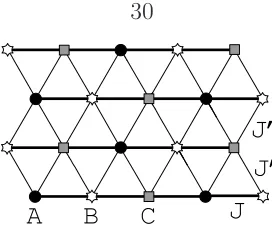
Figure 3.1: Triangular antiferromagnet with coupling constants J and J′ between
nearest-neighbors along horizontal and oblique directions, respectively. Three sublat-tices A, B, and C important in the isotropic case are also labelled.
V
(d)
Y
(b) (c)uud
Spiral (a)
Figure 3.2: Spin orderings on the isotropic triangular lattice in the field, where three arrows refer to three sublattices indicated in Fig. 3.1: a) spiral (non-coplanar um-brella); b, c, d) coplanar Y, uud, and V.
We consider the Heisenberg model in external magnetic field h,
ˆ
H = X
hrr′i
Jrr′ Sr·Sr′ −~h·
X
r
Szr , (3.1)
where Sr is the spin operator on site r and Jrr′ are the nearest-neighbor exchange
couplings. Throughout, we extensively use a hard-core boson picture, mappingS+ r = br and Sz
r = 12 −nr: ˆ
H = −X
hrr′i
trr′ b†rbr′ + H.c.
+X
hrr′i
Jrr′nrnr′ −µ
X
r
nr+ const , (3.2)
trr′ = −
1
2Jrr′, µ=−h+ 1 2
X
r′∈r
Jrr′ . (3.3)
[image:38.612.253.389.53.167.2]The boson hopping amplitudes are negative and therefore frustrated on the triangular lattice, making this a challenging interacting problem.
cap-(a)
(c)
(b)
(d)
n=0 n=1
[image:39.612.183.468.65.323.2]Boson density
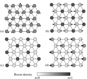
Figure 3.3: Boson interpretation of the spin orderings in Fig. 3.2. Gray scale shows density order hnri, while arrows show superfluid order hb†
ri. a) Spiral is a uniform superfluid phase with rotating phase angles; c)uud is a Mott insulator with√3×√3 CDW order; b,d) Y and V are supersolid phases which contain both charge density and particular superfluid orderings.
in Section 3.4.
3.2
Isotropic triangular antiferromagnet: 6
×
6 Study
In this section, we consider the isotropic triangular Heisenberg antiferromagnet with Jrr′ =J for all nearest-neighbor links. Beginning at density n = 1/3, where we have
an excellent wave function for theuudMott insulator phase of Fig. 3.3c, we construct similarly inspired wave functions for nearby supersolid phases of Figs. 3.3b,d. Next, we describe Bijl-Jastrow-type wave functions for the spiral of Fig. 3.3a and V super-solid of Fig. 3.3d, which perform better for n further from 1/3. We also discuss an alternative construction of the uud state using a det×det (“2-parton”) trial wave function. For the ED calculations, we compute ground state energies for Nb ≤ 12, while Nb ≥13 data is taken from Bernu et al.[68].
We perform all studies at fixed boson number Nb. For each wave function below, we also include a Jastrow factor
Jastrow({nr}) =e−12 P
r,r′urr′nrnr′ (3.4)
with simple choices of pseudopotentialsurr′ providing additional variational freedom.
3.2.1
uud
state at
n
= 1
/
3
At densityn = 1/3, theuudphase is stabilized by quantum fluctuations. We construct a simple boson wave function by using Nb = N/3 orbitals localized around sites Aj, j = 1. . . N/3, from sublatticeA:
|ψuudi = N/3
Y
j=1
X
r
φlocj (r)b†r
!
|0i, (3.5)
φlocj (r) =
1, r =Aj
−α, r = neighbor of Aj 0, otherwise
, (3.6)
h{rk} |ψuudi = Perm
φlocj (ri)
. (3.7)
Trial state Norb
par NJasshort NJaslong Ntotpar E/bond
classical -0.0833
spiral 0 1 2 4 -0.1265
uud 1 0 0 1 -0.1347
1 1 0 2 -0.1354
1 2 0 3 -0.1355
exact -0.1361
Table 3.1: Comparison of uud trial energies for different number of short-range Jas-trow parameters for 12 bosons on a 6×6 cluster. Localized orbitals in the permanent extend only to nearest-neighbor sites with amplitude α, which is single variational parameter in the first listed uud case. The second uudcase has one nearest-neighbor (nnb) Jastrow pseudopotential which is taken to be the same between any pair of nnb sites, while the third case has two such parameters, one for A−B and A−C nnb pairs and the other for B −C nnb pairs, as is appropriate given lattice symmetries of the uud state. We also show trial energy for the spiral state with 4 variational parameters (same as in table 3.3); this state performs poorly compared to the uud state.
boson hopping trr′ < 0. In Eq. (3.7), column j of the Permanent matrix is given
by the j-th orbital (centered on Aj) evaluated on the occupied sites {ri}[76]. One can loosely connect this wave function with a picture starting from the “Ising” limit, Jz ≫ |t|, and perturbatively building in boson kinetic energy effects[72].
Table 3.1 compares the trial energies for different number of variational parame-ters. Excluding any Jastrow factor, the single-parameter trial state already captures the important exchange energies; for example, it is closer to the exact ground state in the zero momentum sector than to the first excited state in this sector (not shown)[68]. Adding a short-range Jastrow factor further improves the trial energy, while longer-range Jastrow parameters are unimportant since correlations in the Mott insulator decay rapidly (see Fig. 3.11 in Appendix 3.B). We see that the simplest localized orbitals extending only to nearest-neighbor sites (and with relatively small amplitude α∼0.23) perform very well, which suggests stronguudorder in the 1/3-filled system. Indeed, for the optimal wave function, we calculate the boson density to be 0.76 on A sites and 0.12 on BC sites.
3.2.2
Y
state at
n
&
1
/
3
Trial state Norb
par NJasshort NJaslong Ntotpar E/bond
classical -0.0961
spiral 0 1 2 4 -0.1424
Y 1 0 0 1 -0.1461
1 1 0 2 -0.1477
1 2 0 3 -0.1478
exact -0.1489
Table 3.2: Comparison ofY trial energies for different number of short-range Jastrow parameters for 13 bosons on a 6×6 cluster. The Y state is constructed by adding one boson to the uud state as described in the text; we allowed the same variational parameters as in the uud case in Table 3.1. We also show trial energy for the spiral state with 4 variational parameters, which has higher energy than the Y state.
bosons to an extended orbital on BC:
|ψYi = X
r
φextBC(r)b†r
!Nb−N/3
|ψuudi , (3.8)
φextBC(r) =
+1, r ∈B
−1, r ∈C 0, r ∈A
(3.9)
Just as in the uud case, the wave function can be written as an Nb×Nb permanent. The first N/3 columns contain the same φloc
j orbitals as in the uud state, while the remaining Nb−N/3 columns all contain the extended orbital φext
BC residing on the B and C sublattices. The alternating signs of the extended orbital are appropriate for bosons hopping on the BC honeycomb with trr′ < 0. Nearest-neighbor contacts on
BC are suppressed by adding a Jastrow factor.
Table 3.2 compares the Y energy against spiral and ED energies for 13 bosons on the 6×6 cluster. Our Y state is close to the ED ground state from Bernu et al.[68]; thus, the trial energy is below the first excited state in the same sector (not shown), while the spiral is significantly higher.
can-Trial state Norb
par NJasshort NJaslong Ntotpar E/bond
classical -0.1250
Y 1 1 2 4 -0.1774
spiral 0 1 0 1 -0.1728
0 1 0 2 -0.1791
0 1 2 4 -0.1795
exact -0.1868
Table 3.3: Comparison of spiral energies for different number of variational parame-ters for 18 bosons on a 36-site cluster. The extended orbital of the spiral state has amplitudes 1, ei2π/3, andei4π/3 for sites on sublatticesA, B, andC respectively. The first spiral case has one nnb Jastrow pseudopotential which is taken to be the same between any pair of nnb sites, while the second spiral case has an additional parame-ter γ for the Huse-Elser phase factor. The third case has two more parameters wand p for a long-range pseudopotential w
|i−j|p between any pair of sites i and j. We also show trial energy for the Y state with 4 variational parameters, which has slightly higher energy than the spiral state.
cellations from alternating superfluid order parameter on theB andC sublattices[75]. In particular, just as in the uud case, we can not construct Bijl-Jastrow-type wave function for the Y state.
3.2.3
Spiral state at
n
.
1
/
2
At half-filling, the 120◦magnetically ordered state (spiral) is believed to be the ground
state. We use Huse and Elser wave function[14], which generalizes Bijl-Jastrow-type wave function by including complex 3-body terms, to accurately describe the corresponding superfluid state of bosons near half-filling. In this wave function, all the bosons reside on an extended orbital,
|ψSi=eiPijkγijk ninjnk X r
ei ~Q·~r b†r
!Nb
|0i, (3.10)
with Q~ = (4π/3,0). Despite frustration, the bosons gain some kinetic energy while hopping along any lattice link. Nearest-neighbor contacts are suppressed by adding a long-range Jastrow factor. The three-body phase factor, which respects the symme-tries of the classical state, serves as an additional variational parameter. For details, the reader is referred to the original Ref. [14].
Trial state Norb
par NJasshort NJaslong Ntotpar E/bond
classical -0.0683
spiral 0 1 2 4 -0.1081
Vperm 1 0 0 1 -0.1141
1 1 0 2 -0.1153
1 2 0 3 -0.1154
exact -0.1161
Table 3.4: Comparison ofVpermenergies for different number of variational parameters for 11 bosons on a 36-site cluster. The Vperm state is constructed by removing one boson from theuudstate as described in the text, and the parameters here are of the same type as in the uudcase in Table I. We also show trial energy for the spiral state with 4 variational parameters, which has higher energy than the Vperm state.
that the 18-boson spiral energy is only slightly lower than the Y energy. This is perhaps not surprising since the classical 120◦ order may be viewed as the spiral
or Y-shape order depending on the plane’s orientation. A recent variational study using different constructions of the spiral and Y states obtained −0.1827 for their many-parameter spiral state, which is also lower than theirY trial energy by a small amount similar to that in our study[62]. Other recent works[75, 74] observed an abrupt change from the spiral to Y supersolid as the spin anisotropy is varied through the Heisenberg point. In principle, thinking in terms of wave functions, the spiral and Y can be distinct phases with different postulated symmetry breaking also in the SU(2)-invariant model. However, this could also be a plane reorientation transition, and the closeness in energy of the Y trial states reflecting their ability to capture the 120◦ spiral order.
3.2.4
V
state at
n
.
1
/
3
Let us now consider densities slightly less than 1/3. We start from the uud state and picture it as a filled A sublattice. An appealing scenario is to introduce holes and let them move around onA and condense. We automatically retain charge order selecting the A sublattice vs. B and C. The condensation of holes on the A gives boson superfluid order there and by proximity effect also on theB and C sublattices. Since tAB =tAC <0, we expect the phase angle on the BC to be shifted by π from the A. The resulting supersolid is precisely the V state.
function with a simpler amplitude given by a single permanent,
h{rk} |ψVpermi= Perm
φloc
1 (r1) . . . φlocN/3(r1) ... . .. ... φloc
1 (rNb) . . . φ loc N/3(rNb) 1 . . . 1
... . .. ... 1 . . . 1
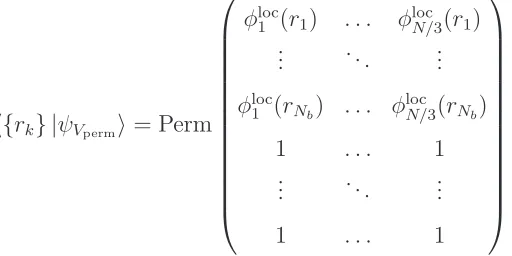
. (3.11)
[image:45.612.186.442.105.233.2]The first Nb rows contain the localized orbitals of the uud construction evaluated at the boson positions, while the remainingN/3−Nbrows are filled with 1-s correspond-ing to “zero wavevector” condensate of holes (see Appendix 3.A for details).
Table 3.4 shows the Vperm energy for 11 bosons on the 6×6 cluster. Being a descendant of the excellent uudstate, even with no Jastrow factor theVperm performs very well and lies roughly half-way between the ground state and the first excited state with the same quantum numbers (the latter is not listed in the table). In particular, the Vperm clearly wins over the spiral superfluid with uniform density. Just as in the uud case, adding simple short-range Jastrow parameters further improves the trial energy of the Vperm state. At this stage, we did not include long-range Jastrow pseudopotentials, which would be needed for a correct long-wavelength description[77] of superfluid correlations in the V phase.
The Vperm state gives our best variational energies for Nb = 6, . . . ,11. In Ap-pendix 3.B, we measure properties of this state and verify the superfluid order with opposite signs on the A and BC sublattices as anticipated above.
3.2.5
V
state at
n
≪
1
/
3
Trial state Norb
par NJasshort NJaslong Ntotpar E/bond
classical 0.13542
spiral 0 1 2 4 0.12885
VBJ 1 0 0 1 0.13216
1 1 0 2 0.12913
1 1 2 4 0.12871
exact 0.12845
Table 3.5: Comparison ofVBijl−Jastrowtrial energies for different number of variational parameters for 2 bosons on a 36-site cluster. The

![Figure 2.3: The Schwinger boson ansatze from Ref. [40], where Aij = 1 if an arrowpoints from site i to a nearest-neighbor site j, −1 for the opposite direction, and zerofor all further neighbors](https://thumb-us.123doks.com/thumbv2/123dok_us/16090.1178/28.612.256.395.53.240/schwinger-arrowpoints-nearest-neighbor-opposite-direction-zerofor-neighbors.webp)