Algorithm for MTF estimation by histogram modeling of an edge

Rochester Institute of Technology

RIT Scholar Works

Theses Thesis/Dissertation Collections

2001

Algorithm for MTF estimation by histogram

modeling of an edge

Brian Perry

Follow this and additional works at:http://scholarworks.rit.edu/theses

This Thesis is brought to you for free and open access by the Thesis/Dissertation Collections at RIT Scholar Works. It has been accepted for inclusion in Theses by an authorized administrator of RIT Scholar Works. For more information, please [email protected].

Recommended Citation

SIMG-503

Senior Research

Algorithm for MTF Estimation by

Histogram Modeling of an Edge

Final Report

Brian Perry

Center for Imaging Science Rochester Institute of Technology

Table of Contents

I. Abstract……… 3

II. Copyright………. 4

III. Acknowledgment………. 5

IV. Background……….. 6

V. Experimental Design and Methods……….. 8

VI. Results……….. 11

VII. Discussion and Conclusion……….. 15

I. Abstract

The Modulation Transfer Function, or MTF, is a property of an imaging system

that describes the effect that the system has on the sharpness of an object. It is an

important image quality metric that has applications in almost every major Imaging

Science application. The traditional method of determining the MTF, however, relies on

aligning an edge perpendicular to the scan line that will be used to take the measurement.

This may not always be a convenient orientation for your experiments. It is hypothesized

that there is a relationship between the histogram of the scan line (regardless of its

position) and the MTF of the system. This research project will explore this relationship

II. Copyright

Copyright © 2001

Center for Imaging Science

Rochester Institute of Technology

Rochester, NY 14623-5604

This work is copyrighted and may not be reproduced in whole or part without permission of the Center for Imaging Science at the Rochester Institute of Technology.

This report is accepted in partial fulfillment of the requirements of the course SIMG-503 Senior Research.

Title: Algorithm for MTF Estimation by Histogram Modeling of an Edge. Author: Brian Perry

Project Advisor: Dr. Jonathan Arney SIMG 503 Instructor: Anthony Vodacek

III. Acknowledgment

I want to extend a special thanks to Dr Jonathan Arney for his outstanding help

and guidance in this Research Project in his role as my Research Advisor. I would also

like to thank him for his support and guidance in my studies here at the Center for

IV. Background

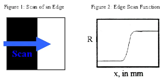
The traditional method of calculating the MTF involves taking an edge scan of an

image perpendicular to the edge as illustrated in Figure 1. The scan averages all the

pixels in the vertical direction parallel to the edge, and the result is a graph of reflectance

versus position as shown in Figure 2.

Figure 2 is also referred to as the edge spread function. This function gives a very good

description of what the line scan looks like. In this case you can see that the edge doesn’t

appear to be an instantaneous transition, but in fact it is a gradual transition from Black

through the grays to white. This begins to give us some information about how the

imaging system treats edges.

The next step is to take the derivative of the edge scan function.

dx dR x Function Spread

Line ( )= (1)

The resultant Line Spread Function, illustrated in figure 3, gives us a function that

The line spread function is the probability density function for the location of the edge in

the output image. In an imaging system with perfect resolution, this function would be a

delta function of zero width.

The Modulation Transfer function, MTF(ω), is the line spread function

represented in the frequency domain, ω. In this new space the MTF provides us

information on what frequencies are attenuated by the imaging system. In order to get

from the Line Spread Function to the MTF you have to use a Fourier Transform function

as illustrated in equation 2.

( )

{

}

MTFω = (2)

The value of MTF(ω) in Figure 4 is the fraction of the contrast of the image that is

attenuated by the imaging system for image features at each spatial frequency, ω. In this

particular graph the low frequencies get through with little attenuation but quickly drop

off at higher frequencies. In this way the MTF is an important tool in describing how an

V. Experimental Design and Methods

The main problem that this project was designed to solve involves finding the

MTF of images in which the edge is not perfectly perpendicular.

If the MTF were taken of these two images, one would find that the MTF of the second

image appears lower, even though both images are from the same system and therefore

must have the same MTF. The challenge is to find a technique that will produce the same

MTF regardless of the orientation of the edge. One might, for example, try to develop a

way to locate the perpendicular direction and perform a slant scan, or to adjust the image

to make the edge perpendicular to the direction of the scan. The approach taken in this

project was to abandon the scan process and to show that the edge scan function, R(x) vs

x, can be calculated directly from the gray level histogram of the image regardless of the

orientation of the edge.

Traditional wisdom in imaging science holds that the gray level histogram of an

image contains no spatial information. This, however, is not entirely true. The histogram

by itself is not sufficient to give spatial information, but with additional information

about the spatial characteristics of an image, it is often possible to extract quantitative

spatial information from the histogram. The additional information needed to constrain

The additional information is that the image is an edge. This means the gray values

increase monotonically across the image in the direction perpendicular to the edge.

Figures 5 and 6 demonstrate how the histograms of a sharp and a smooth edge

must differ. The gray levels increase in the histogram from left to right. This also

represents a monotonic spatial motion across the edge in the perfectly orthogonal scan

direction. The differences between the histograms of the sharp and soft edges is clearly

shown in Figures 5 and 6. There are far fewer mid-tone gray values in the sharp edge.

Indeed, as will be shown below, the shape of the mid-tone gray portion of the histogram

is a direct measure of the edge sharpness and the line spread function.

The histogram of an edge image can be interpreted as being proportional to the

rate of change of position with respect to the change in R.

dR dx R

Histogram( )= (3)

By integrating the Histogram we find the Cumulative Distribution Function.

∫

The CDF(R) function is the location along the edge according to equation (5), and the

inverse of Figure 7 is the edge function, R(x) versus position, x.

) ( )

(R CDF R

x = (5)

Experimentally, we rotate Figure 7 ninety degrees clockwise and obtain the line spread

function of Figure 2. This is the line scan function for x as the scan direction that is

orthogonal to the edge. We should then be able to derive the MTF using the steps outline

VI. Results

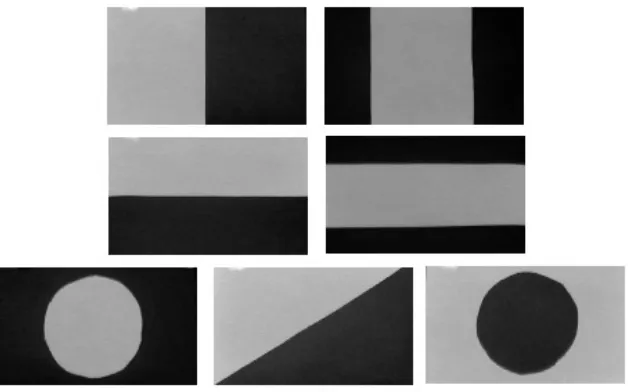
We designed 7 different geometries to test our theory. All of the images contained

approximately the same amount of light and dark space. Figure 8 shows the 7 different

targets: Single Vertical Edge, Double Vertical Edge, Single Horizontal Edge, Double

Horizontal Edge, Single Diagonal Edge, Light Circle on a Dark Background and Dark

Circle on a light background.

Figure 8: The different test images

Figure 9 shows the results of our histogram analysis for the single vertical edge.

Our histogram method produced line (A), and line (B) was produced by the traditional

method. This shows that the histogram method produces a remarkably similar result to

the traditional edge method. We would expect this to happen considering that our theory

is based on the assumption that the image is increasing monotonically in the horizontal

Figure 9: Comparison of the histogram analysis, Line (A), with the traditional edge analysis, Line (B). Responsivity is the MTF for the traditional edge analysis, Line (B), but it is the response function F(ω) for the histogram analysis technique. The frequency

at 1/2 response is the same for both.

0 50 100 150 200

1

0 0.5

(A) (B)

Frequency ω in cycles per field of view

Responsivity _ω

1/2 = 78 cy/fov

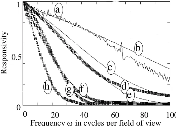
Figure 10: The MTF for the traditional edge scan technique (a), and the response functions for the histogram technique applied the images in Figure 1. Lines (b) through

(h) are respectively the single vertical, double vertical, diagonal, single horizontal, double horizontal, dark circle, and light circle.

Responsivity

1

0.5

0

0

0

20

40

60

100

Figure 11 shows the results of the histogram analysis applied to all of the test

edges of Figure 8, and clearly the nature of the edge has a significant effect on the results

of the analysis. Figure 11 indicates that as the length of the edge increases, the response

curve shifts to lower frequency. Table I summarizes the effect of edge length on the

wavelength (1/frequency) at a response of 0.5.

Table I: Summary of edge length and 50% wavelength (L and λ1/2 ) for the images in Figure 8.

Type of Edge

Image

Edge Length (pixels)

λ

(mm)

One Vertical

374

7.0

Two Vertical

635

16.2

One Horizontal

748

15.5

Two Horizontal

1270

45.4

One Diagonal

737

12.5

Dark Circle

1000

28.9

White Circle

1000

28.9

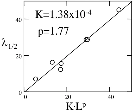
Figure 11: Wavelength at 50% response, λ1/2 , versus a power

function of the edge length, K.Lp, from the data in Table I.

0 20 40

0 20 40

λ

K

L

K=1.38x10

Figure 11 illustrates the data in Table I. Empirically it was found that the data fit

well with equation (6) with constants K = 0.000138 and p = π .

p

K

L= ⋅(λ1/2) (6)

Using this equation, we can derive a general expression for converting the histogram

response function, F(ω), to an estimate of the MTF(ω) function. We do this by

assuming, based on experimental evidence, that F(ω) = MTF(ω) for the single vertical

edge of length Lo. Then it can be shown from equation (6) that the MTF(ω) function is

given by equation (7).

⎥ ⎥ ⎦ ⎤ ⎢ ⎢ ⎣ ⎡ ⎟ ⎠ ⎞ ⎜ ⎝ ⎛ ⋅ = P o L L F

MTF(ω) ϖ (7)

The advantage of using a test target with multiple edges is in the increased data available

for estimation of the shape of the MTF. By using equation (7), the multiple edge target

can be used with the histogram analysis technique to estimate the MTF. However, it is

important to recognize that equation (7) is an empirical expression found by fitting

experimental data. It would be very useful to derive a justification for equation (7) from

VII. Discussion and Conclusion

In this experiment we demonstrated that it is possible to arrive at the modulation

transfer function by having only a histogram and an assumption about image

composition. We know that this technique is not sensitive to small errors in the edge

orientation. We were able to derive an expression to describe the relationship between

wavelength and edge length in this set of images. Our data can be calibrated to a wide

range of edge types ranging from a single vertical edge to a circle. In addition, this

project has exposed some issues that deserve more research attention.

• The Theoretical Origin of Equation 6

We are still attempting to understand the theory that dictates equation 6. The

constant K depends on the experimental field of view and must be determined by

calibration every time the instrument is set up. It seems logical that the power p should

be a universal characteristic, and we hope that future research will help to derive the

theory that gives us the value of p.

• Noise

Experimental noise seems to manifests itself differently in this analysis, and we

still don't have a full evaluation of the effect of noise. The histogram analysis technique

assumes that gray level changes monotonically with location orthogonal to the edge.

Random fluctuations in gray level are treated experimentally as monotonic gray level

and after the location of the edge. Presumably it will be possible to correct for such

random noise by a simple slope adjustment, but further research will be needed to fully

develop this analytical technique of MTF estimation.

• What are the Boundaries of this Technique

We know already that there will be limitations to this technique. For example, if

the edges are enhanced in a way that results in a non-monotonic change in gray level with

location, this technique will incorrectly reconstruct the MTF. We need to know what

other limits may exist in this analysis.

Although a number of uncertainties remain regarding the extraction of spatial

information form the histogram, this project has demonstrated that histograms, with

limits, do have the potential of providing useful spatial information. Thus, the major

contribution of this project is to demonstrate that additional research in this area would be

VII. References

Arney, J.S and Wong, Yat-Ming, “Histogram Analysis of the Microstructure of

Halftone Images.” IS&T’s 1998 PICS Conference