A fully Bayesian approach to shape estimation of objects from tomography data using MFS forward solutions

(1)

This is a repository copy of

A fully Bayesian approach to shape estimation of objects from

tomography data using MFS forward solutions

.

White Rose Research Online URL for this paper:

http://eprints.whiterose.ac.uk/79318/

Version: Accepted Version

Article:

Aykroyd, RG, Lesnic, DL and Karageorghis, A (2015) A fully Bayesian approach to shape

estimation of objects from tomography data using MFS forward solutions. International

Journal of Tomography and Simulation, 28 (1). 1 - 21. ISSN 0972-9976

[email protected] https://eprints.whiterose.ac.uk/ Reuse

Unless indicated otherwise, fulltext items are protected by copyright with all rights reserved. The copyright exception in section 29 of the Copyright, Designs and Patents Act 1988 allows the making of a single copy solely for the purpose of non-commercial research or private study within the limits of fair dealing. The publisher or other rights-holder may allow further reproduction and re-use of this version - refer to the White Rose Research Online record for this item. Where records identify the publisher as the copyright holder, users can verify any specific terms of use on the publisher’s website.

Takedown

If you consider content in White Rose Research Online to be in breach of UK law, please notify us by

(2)

A fully Bayesian approach to shape estimation of objects

from tomography data using MFS forward solutions

Robert G. Aykroyd1_{, Daniel Lesnic}2 _{and Andreas Karageorghis}3

1_{Department of Statistics}

University of Leeds Leeds, LS2 9JT, UK [email protected]

2_{Department of Applied Mathematics}

University of Leeds Leeds, LS2 9JT, UK [email protected]

3_{Department of Mathematics and Statistics}

University of Cyprus Nicosia, Cyprus [email protected]

ABSTRACT

(3)

1 INTRODUCTION

Inverse problems occur in a wide range of practical applications in geophysics, industry and medicine – see Stuart (2010) for a Bayesian perspective of inverse problems. For example in electrical tomography, voltages are recorded between multiple electrode-pairs attached to the boundary and the aim is to reconstruct the interior conductivity distribution – a review of statistical modelling for such examples can be found in Watzenig and Fox (2009). The standard method of analysis involves domain discretization and the use of the finite element method. This, however, inevitably leads to an ill-posed inverse problem demanding regular-ization. For examples of this approach to electrical impedance tomography (EIT), see West et al. (2004; 2005) and references therein. In the following sections an alternative approach is proposed. A parametric model of the inclusion will be defined and brief details of the method of fundamental solutions (MFS) will be given. Then, Bayesian statistical modelling will be dis-cussed with specific examples given and an outline of the Markov chain Monte Carlo (MCMC) method presented – for a detailed theoretical discussion of the MCMC method see, for exam-ple, Geyer (2011) and Brooks et al. (2011). To demonstrate the proposed approach a series of numerical simulations are described which highlight the flexibility of the modelling and estima-tion procedures.

2 MATHEMATICAL MODELLING

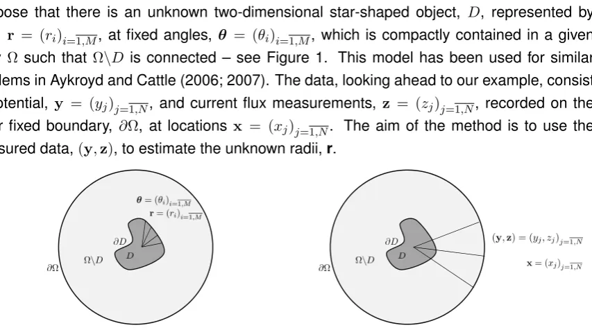
[image:3.595.93.520.425.663.2]

Suppose that there is an unknown two-dimensional star-shaped object, D, represented by radii, r = (ri)_i=1,M, at fixed angles, θ = (θi)i=1,M, which is compactly contained in a given body Ω such that Ω\D is connected – see Figure 1. This model has been used for similar problems in Aykroyd and Cattle (2006; 2007). The data, looking ahead to our example, consist of potential, y = (yj)j=1,N, and current flux measurements, z = (zj)j=1,N, recorded on the outer fixed boundary, ∂Ω, at locations x = (xj)_j=1,N. The aim of the method is to use the measured data,(y,z), to estimate the unknown radii,r.

Figure 1: Diagram of star-shaped object model (left) and data measurements (right).

The data model defines the measurements on ∂Ωin terms of exact values of the potential,u, and the current flux,∂u/∂n, combined with additive Gaussian noise, that is,

yj =u(xj) +ϵj, zj =

∂u

(4)

where n is the outer unit normal to the boundary ∂Ω, and the noise (ϵj)_j=1,N and (ζj)j=1,N follow independent normal distributions, with zero means and variancesσ2

yandσ2z, respectively, andusatisfies the Laplace equation inΩ\D. Further, ifDis a rigid inclusion thenu= 0on∂D, otherwise ifDis a cavity then∂u/∂n= 0on∂D. We can also have thatDis an inclusion with a different conductivity than that of the backgroundΩ\Din which case transmission conditions are applied at the interface∂D.

The values of the potential and current flux on ∂Ωare calculated using the MFS, see Borman et al. (2009) and Karageorghis et al. (2011; 2013), as a linear combination of fundamental solutions of the governing Laplace equation

u(c,ξ, xj) = 2M ∑

k=1

ckG(ξk, xj),

∂u

∂n(c,ξ, xj) =

2M ∑

k=1

ck

∂G

∂n(ξk, xj), j = 1, N , (2.2)

whereG(ξ, x) =− 1

2πlog|ξ−x|is the fundamental solution in two-dimensions of the governing Laplace equation and ξ = (ξk)k=1,2M are sources which are located on pseudo-boundaries inside the rigid object D and outside the outer fixed boundary ∂Ω. We also need to impose thatDis a rigid inclusion, that isu= 0on∂D, which can be rewritten as

2M ∑

k=1

ckG(ξk,(ricos(θi), risin(θi))) = 0, i= 1, M . (2.3)

Notice that the MFS introduces an additional 2M unknown coefficients,c = (ck)_k=1,2M, which must be estimated in addition to theM radii,r= (ri)_i=1,M from the system given by equations (2.3) and those obtained by fitting (2.2) to match the Cauchy data measurements (2.1), that is,

2M ∑

k=1

ckG(ξk, xj) =yj, j= 1, N , (2.4)

and

2M ∑

k=1

ck

∂G

∂n(ξk, xj) =zj, j= 1, N . (2.5)

A geometric nonlinear constraint that D is compactly contained in Ω can also be imposed. Altogether, equations (2.3)–(2.5) form a system of(2N+M)equations with3Munknowns. Out of these equations, (2.4) and (2.5) are linear in c, whilst equation (2.3) represents nonlinear equations. The tomographic inverse rigid inclusion problem is nonlinear and ill-posed, but provided u

∂Ω ̸≡ 0 the solution is unique (Haddar and Kress, 2005). The solution may not exist, but even if the solution exists it is not stable with respect to the noise in the Cauchy data measurements defined in equation (2.1).

3 STATISTICAL MODELLING

(5)

modelling, see Gelman et al. (2003), and for applications of Bayesian modelling in electrical tomography problems, see West et al. (2004; 2005) and Aykroyd and Cattle (2006; 2007).

With data (y,z), and assuming (conditional) independence of yandzgivenrandc, then the appropriate form of the likelihood is:

l(y,z|r,c) =l(y|r,c)×l(z|r,c). (3.1)

The likelihood quantifies both the inaccuracies in the measuring equipment and other uncon-trolled influences. From (3.1), the likelihood ofygivenrandcis

l(y|r,c) = (2πσ_y2)−N/2_exp {

− 1

2σ2 y

||y−yˆ(r,c)||2 }

, (3.2)

whereyˆ(r,c) = (ˆyj(r,c))j=1,N are fitted values assuming inclusion radiirand MFS coefficients

c. The structure of the likelihood ofz givenrandcis identical to (3.2), except thatz replaces

y,ˆzreplacesyˆ andσ2

z replacesσy2.

Estimating from the likelihood alone may not be possible due to the non-linear relationship between the radii,r, and the data, and the ill-posed nature of the problem in terms of the MFS coefficients, c. In a standard approach, progress can be made by imposing regularization. This leads to a numerical approach which will produce point estimates, but there will be no information about confidence, that is, about the precision of the point estimates. Here an alternative approach is adopted based on the widely used Bayesian modelling framework. The key addition to the modelling is to consider prior distributionsfor the model parameters which quantify specific expert opinion or more vague knowledge of the relative ranking of the various alternatives.

It is assumed that there is some knowledge of the values, or relationship between, the model parametersrand c. In the examples considered here we expect the boundary to vary gently around the object, which suggests smoothing, leading to a prior distribution such as

π(r|βr) =

1 (2πβ2

r)M/2

exp

{ − 1

2β2 r

||∇r||2 2

}

, (3.3)

which uses a 2-norm, and hence corresponds to a Gaussian distribution, or

π(r|βr) =

1 (2βr)M

exp

{ −1

βr ||∇r||1

}

, (3.4)

which uses the 1-norm, and hence gives a Laplace distribution. In each case,||∇r||qq =∑|ri−

ri−1|

q_{, with periodic boundary, and}_β

rdefines the amount of variability between adjacent radii.

The whole prior modelling can be repeated for the MFS coefficients producing prior distribution,

π(c|βc), forc. Here, the same first-order smoothing prior distribution will be used, but the range of alternatives is still available and there is no requirement for this to be of the same type as for the radii.

Bringing the likelihood functions and prior distributions together gives the corresponding pos-terior distributionas the product of likelihood and prior distribution

(6)

,

r

,

r

,

rrrr

[image:6.595.157.474.80.256.2]

Model 1 Model 2 Model 3

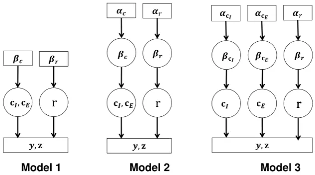
Figure 2: Hierarchical relationship between data, model parameters and hyper-parameters.

The hierarchical structure of this model is represented in the directed graph in Figure 2 (left). The boxed variables are fixed data and prior parameters whereas the circled variables are to be estimated. The arrows indicate causal relationships.

Now, of course, the prior parameters, βr and βc, are also unknown and hence should be included in the modelling process. Here thehyper-prior distributionforβris taken as

π(βr) =α2r exp {

−α2_r/β_r2}

. (3.6)

This is an example of the, widely used, inverse-gamma prior for a variance parameter (Gelman, 2006). The value of thehyper-parameter,αr, can be fixed at a reasonable value chosen during initial trials. In addition, there will be a similar prior, π(c|βc), forc and hyper-prior distribution forβc with a hyper-parameterαc. This leads to the full posterior distribution as the product of likelihood, prior and hyper-prior distributions

Figure 2 (centre) illustrates the hierarchical relationship between the model variables.

Taking the modelling one final step further, it is entirely reasonable to allow separate prior distributions, π(cI|βc_I) and π(cE|βc_E), for the two sets of MFS coefficients in (2.2), that is,

cI = (ck)k=1,M, those associated with the interface∂D, andcE = (ck)k=M+1,2M, those associ-ated with the outer boundary∂Ω. This then also suggests corresponding separate hyper-prior distributionsπ(cI)andπ(cE), with separate hyper-prior parameters,αcI andαcE. Again these

hyper-prior parameters will be fixed at reasonable values chosen during initial trials. The result-ing posterior distribution is again the product of likelihood, prior and hyper-prior distributions

(7)

4 MARKOV CHAIN MONTE CARLO ESTIMATION

The Markov chain Monte Carlo (MCMC) approach is now widely used for many Bayesian sta-tistical estimation problems in situations were model complexity and parameter dimensionality make other procedures infeasible – see, for example, Gamerman and Lopes (2006) and Liu (2008). The procedure has come to mean much more than an alternative numerical method. In particular, the approach allows a deeper exploration of the posterior distribution than permitted by other approaches.

The MCMC approach gives a framework which can be used to design tailor-made iterative al-gorithms for many estimation problems. In particular, a resulting algorithm is used to produce a correlated sample from some target statistical distribution – usually the posterior distribution in a Bayesian analysis. Specifically, the transitions in the Markov chain are designed so that an equilibrium distribution exists and is equal to the target distribution. If the transitions are designed well, then after an initial transient period, referred to as burn-in, the remaining sam-ple will have the same statistical properties as a samsam-ple obtained directly from the posterior distribution. The only exception is that, by the very nature of a Markov chain, there will be correlation within the sample which must be taken into account when the algorithm output is summarised. If transitions are designed badly however, then the initial transient period could be long and the within sample correlation could be high. This means that the algorithm is inefficient and would require larger samples to achieve acceptable accuracy and precision.

Our particular implementation is now described. Suppose, that all the model parameters are stored in a single vector, Θ = (Θi)i=1,p. Examples of this are, Θ = (r,c),Θ = (r,c, βr, βc) and Θ = (r,c, βr, βcI, βcE) – these are the three cases illustrated in Figure 2. Starting from

an arbitrary value, Θ0, K random walk transition steps are performed based on Gaussian perturbations. At each step,k= 1, K, the proposed value is accepted with a probability which depends on a posterior ratio. The algorithm is summarised in Figure 3. The statement and implementation of the algorithm are straightforward and a sensible choice for the variance,τ2

, in the proposal distributions can be made from initial experimentation.

Set an initial value forΘ= (Θ)_i₌₁_,p, call thisΘ0

Repeat the following steps fork= 1, K

Repeat the following steps fori= 1, p

Propose new valueΘk_i = Θk−1

i +N(0, τ2) Evaluateα= min{

1, π(Θk|y,z)/π(Θk−1|_y,_z)}

Generateufrom a uniform distribution,U(0,1)

Ifα > uthen accept the proposal, otherwise reject and setΘk= Θk−1

End repeat End repeat

Discard initial values and use remainder to make inference.

(8)

As this is a very simple estimation problem, an equally simple random walk proposal is very likely to work well. When considering more complex estimation problems, particularly with many parameters, more careful consideration may be needed. The efficiency of the algorithm, however, is heavily dependent on the choice of the proposal scheme.

When choosing a value for τ2_{, it is important to realise that both low and high values lead to} long transient periods and highly correlated samples and hence unreliable estimation. A rea-sonable proposal variance can be chosen adaptively during the early burn-in period, and it has been proven theoretically that for a wide variety of high-dimensional problems an acceptance rate of 23.4% (Roberts et al., 1997) is optimal. Further, if different types of parameter are be-ing estimated, then it may be appropriate to have a separate proposal variance for each type. Further, it is wise to also check Markov chain paths and to calculate sample autocorrelation functions. For good estimation the paths should look “random” and the autocorrelation func-tions be close to zero for all except small lags. For suggesfunc-tions on judging the appropriate size of MCMC samples, and other convergence issues, see Raftery and Lewis (1995), Cowles and Carlin (1996) and Geyer (2011).

Once the sample has been generated from the posterior distribution, a number of possible es-timators are available. One choice is the posterior mean, which can be estimated by the mean of the sample collected after a suitable burn-in period to allow the chain to reach equilibrium. The whole MCMC sampling ethos encourages the investigation of a variety of summary mea-sures, and not only mean and variance. Instead the sample can be used to calculate interval estimates using sample percentiles, or in fact the whole of the posterior distribution can be examined. Also, it is usual not to assume normality of the sampling distributions of the various quantities being estimated, but instead the sample histogram is used to estimate the unknown distribution. In the following numerical results section a variety of output will be shown, but as a minimum it is usual to examine the histogram of the sampling distributions and to form credible intervals using the percentage points of the corresponding sampling distribution. For applications of MCMC methods to electrical tomography, see West et al. (2004; 2005) and Aykroyd and Cattle (2006; 2007).

5 NUMERICAL RESULTS

5.1 Preliminary

In this section part of a series of numerical experiments based on simulated data will be re-ported. Three true object geometries forDwill be considered, namely: (i) a circle of radius0.5

centred at the origin given by the radial parameterization

r(θ) = 0.5, θ∈[0,2π); (5.1)

(ii) a bean-shaped obstacle given by the radial parameterization (Ivanyshyn and Kress, 2006),

r(θ) = 0.5 + 0.4 cos(θ) + 0.1 sin(2θ)

(9)

and (iii) a round-cornered rectangle given by the radial parameterization (Ivanyshyn, 2007)

r(θ) = 2 3

[

sin10(θ) +

(

2 3cos(θ)

)10]

,

−0.1

θ∈[0,2π); (5.3)

each of these being contained in the unit discΩ.

First we determine the current flux data,∂u/∂n, on∂Ωby solving the direct Dirichlet problem

∇u= 0 inΩ\D, (5.4a)

u= 0 on∂D (5.4b)

u(1, θ) = exp(

−cos2(θ))

on∂Ω ={(1, θ)|θ∈[0,2π)}, (5.4c)

using the MFS with M = 500 degrees of freedom. The boundary potential and current flux measurements were then selected atN = 30equally-spaced points on the outer fixed bound-ary∂Ω. Data, as defined in equations (2.1), was then produced by addition of Gaussian noise withσy =σz = 0.01(corresponding to a signal-to-noise ratio of 1%). We also takeM = 50such that the discretised problem defined in equations (2.3)–(2.5) is underdetermined as it contains

M+ 2N = 110equations with3M = 150unknowns. Of course, by increasingnto50or beyond we obtain the determined and the overdetermined situations. For more details of applying the MFS to these three scenarios, see Smyrlis and Karageorghis (2009). The contraction and dila-tion parameters,η andχ, entering the boundaries{χr(θ)|θ∈[0,2π)}andη∂B(0; 1), on which the sources(ξk)_k=1,2M are positioned, are taken to beη= 1.8andχ= 0.9.

The first section below reports a pilot study to understand the effects of smoothing on the estimation of the MFS coefficients, as well as on the rigid inclusion shape. Then the second section considers full model estimation using Gaussian prior distributions and the final section shows results of full estimation using Laplace prior distributions.

5.2 Understanding the influence of the prior distribution

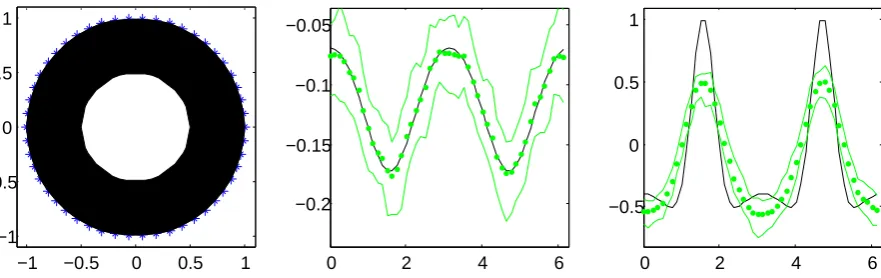
In the first set of examples the true object, D, is taken as the disk of radius 0.5 centred at the origin as parameterised by equation (5.1). The simplest possible model includes a single unknown radius,r, along with unknown MFS coefficients,c. Figure 4 shows the object recon-structed (left), without prior information, using the radius estimated as the mean of the posterior sample. Also shown are the estimated MFS coefficients (centre and right) surrounded by 95% credible intervals. In all the relevant figures these coefficients are plotted as functions ofθ.

The posterior estimate of the radius is 0.4997, compared to the true value of 0.5, with an estimated standard deviation of0.00107. The estimated MFS coefficients follow the true values, which were obtained from the MFS direct problem solution and are shown in all relevant figures as a continuous dark line, but clearly those associated with the interface source points (centre) show substantially more variability between values and greater uncertainty in the estimates than those associated with the outer boundary points (right).

(10)

param-−1 −0.5 0 0.5 1 −1

−0.5 0 0.5 1

0 2 4 6

−0.2 −0.15 −0.1 −0.05

0 2 4 6

[image:10.595.70.519.144.281.2]

−0.5 0 0.5 1

Figure 4: Circular inclusion and circle model fitted with no prior information: fitted circle (left) and MFS coefficients (with credible intervals) associated with the interface (centre) and outer boundary (right).

−1 −0.5 0 0.5 1

0 2 4 6

−0.2 −0.15 −0.1 −0.05

0 2 4 6

−0.5 0 0.5 1

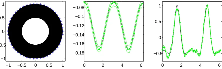
Figure 5: Circular inclusion and circle model with strong prior information (βcI =βcE = 0.01):

[image:10.595.75.516.496.635.2]

(11)

eters βcI = βcE = 0.01. The reconstructed object (left) is indistinguishable from the previous

reconstruction, but the estimated MFS coefficients are very different to those without prior smoothing. The coefficients for the interface (centre) very closely follow the true values and the credible intervals are reasonably constant in width. Notice, however, that overall the width of the credible intervals has not changed dramatically. For the coefficients associated with the outer boundary (right) the variability between estimates has reduced (for example, focus on the region between2and4), but there is a dramatic bias in the estimated values. In particular, the width and height of the peaks is lost. In summary, the coefficients for the interface are well-estimated with this choice of smoothing parameters, but those for the outer boundary are over-smoothed.

The obvious suggestion is to reduce the amount of smoothing by reducing the value of the smoothing parameters. In another experiment, not shown here, the values βcI = βcE = 0.1

[image:11.595.72.517.444.582.2]

were used. The estimates of the coefficients for the interface, however, resemble those without smoothing even though those coefficients for the outer boundary are well estimated. The conclusion from these two experiments is that the coefficients for the interface benefit from more smoothing than those for the outer boundary.

Figure 6 shows the object reconstructed using fixed prior parameters βcI = 0.01 and βcE = 0.1. Clearly, for both sets of coefficients the estimates closely follow the true values and have narrow credible intervals. As well as producing good object reconstruction the process has also produced accurate coefficient estimates which could be easily described. Hence, we conclude that smoothing of the MFS coefficients is worthwhile, but that it is not appropriate to use the same degree of smoothing for the interface and outer boundary coefficients.

−1 −0.5 0 0.5 1

0 2 4 6

−0.18 −0.16 −0.14 −0.12 −0.1 −0.08

0 2 4 6

−0.5 0 0.5 1

Figure 6: Circular inclusion and circle model with separate prior information (βcI = 0.01,

βcE = 0.1): fitted circle (left) and MFS coefficients (with credible intervals) associated with

the interface (centre) and outer boundary (right).

5.3 Full estimation using Gaussian prior distributions

Consider now the full estimation incorporating the hyper-prior distributions and hence including estimation of the prior parameters βcI andβcE. For this, we must specify values for the

hyper-prior parametersαcI andαcE. Here the values of the fixed smoothing parameter values from

(12)

show summaries from the MCMC estimation.

0 0.05 0.1 0.15

0.44 0.46 0.48 0.5 0.52 0.54

0 0.1 0.2 0.3

0 0.1 0.2

[image:12.595.66.527.87.225.2]

0 0.1 0.2 0.3

Figure 7: Circular inclusion and circle model with full posterior distribution and separate prior information (αcI = 0.01and αcE = 0.1): histograms, showing the posterior relative frequency,

for radius (left) and MFS interface (centre) and outer boundary coefficients (right).

−1 −0.5 0 0.5 1

0 2 4 6

−0.18 −0.16 −0.14 −0.12 −0.1 −0.08

0 2 4 6

[image:12.595.69.518.289.425.2]

−0.5 0 0.5 1

Figure 8: Circular inclusion and circle model with full posterior distribution and separate prior information (αcI = 0.01 and αcE = 0.1): fitted circle (left) and MFS coefficients (with credible

intervals) associated with the interface (centre) and outer boundary (right).

Figure 7 shows posterior histograms for the object radius,r, and for the prior parametersβc_I and βc_E. As summaries of this information, posterior estimates (with standard deviations) are

ˆ

r = 0.4992 (0.0024),βˆCI = 0.0116(0.0045), and βˆCE = 0.2457 (0.0891). Clearly, the variation

in the radius is very small indicating that it can be well estimated. Similarly, the smoothing parameter, βcI, for the interface coefficients has low variability. In contrast, the smoothing

parameter for the outer boundary, βcE, has higher variability and slight positive skew. It is

worth noting that the posterior estimate of the smoothing parameter for the interface, βcI, is

close to the prior mean and hence the likelihood has little effect. In contrast, the posterior estimate of the smoothing parameter for the outer boundary, βcE, is not sensitive to the prior

mean value,αcE.

Figure 8 shows the reconstructed object and estimates of the MFS coefficients with credible intervals. The inclusion remains well estimated and, although the MFS coefficient smooth-ing parameters are besmooth-ing estimated, the estimates of MFS coefficients have not significantly changed. This demonstrates that it is possible to successfully estimate the prior smoothing parameters and the inclusion shape together without loss of accuracy.

(13)

[image:13.595.71.519.382.518.2]

equally-spaced angles. The prior parameter for the radii smoothing, βr was fixed at1.0, and the prior parameters for the MFS coefficient smoothing were fixed at the posterior estimates from the previous example, that isβcI = 0.0116andβcE = 0.2457.

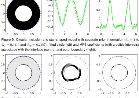
Figure 9 shows the reconstructed inclusion and estimated MFS coefficients. The dataset used is based on a circular true object and so the reconstruction is very accurate. The mean of the posterior radii (with standard deviation) is 0.5012(0.0012). Similarly, the MFS coefficients are well estimated. It is worth noting that the object reconstruction is not sensitive to the value of the prior parameter,βr, but the reconstruction is significantly worse if this smoothing is removed completely from the modelling. Accuracy and variability in the object reconstruction are shown in Figure 10. The estimation errors (left), defined as the difference between the estimated and true radii, are indicated by the very thin region around the inner circle. This shows that the esti-mation errors are very small and are reasonably evenly distributed around the circle. A circular histogram (centre) and circular credible interval (right) aim to describe estimation variability. In the histogram the darker regions indicate the higher frequencies and in the credible interval the thickness of the region indicates the amount of variability. From this, it is clear that the circular histogram tends to exaggerate the slightly non-circular shape of the reconstructed object and hence perhaps the credible interval gives a more reliable representation. These results show that fitting of the star-shaped model to data from a circle truth has been successful.

−1 −0.5 0 0.5 1

0 2 4 6

−0.18 −0.16 −0.14 −0.12 −0.1 −0.08

0 2 4 6

−0.5 0 0.5 1

Figure 9: Circular inclusion and star-shaped model with separate prior information (βr = 1.0,

βcI = 0.0116andβcE = 0.2457): fitted circle (left) and MFS coefficients (with credible intervals)

associated with the interface (centre) and outer boundary (right).

−1 −0.5 0 0.5 1

[image:13.595.66.522.399.721.2]

−1 −0.5 0 0.5 1

Figure 10: Circular inclusion and star-shaped model with separate prior information (βr= 1.0,

βcI = 0.0116 and βcE = 0.2457): estimation errors (left), object boundary histogram (centre)

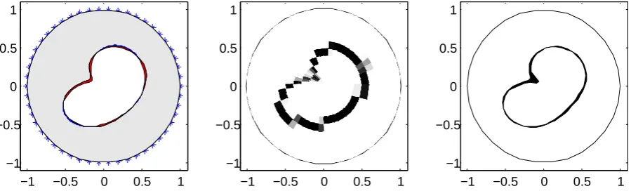
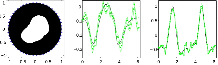
[image:13.595.65.520.562.711.2]

(14)

In the next experiment the star-shaped model is applied for recovering the bean-shaped truth, as defined in equation (5.2), with the prior parameters kept fixed as before. Figure 11 shows the reconstructed object and estimated MFS coefficients for the interface and outer boundary. The rigid bean-shaped inclusion is clearly recovered and MFS coefficients are well estimated without the need for any adjustments.

−1 −0.5 0 0.5 1

0 2 4 6

−0.25 −0.2 −0.15 −0.1 −0.05 0

0 2 4 6

[image:14.595.71.519.154.290.2]

−0.5 0 0.5 1

Figure 11: Bean-shaped inclusion and star-shaped model with separate prior information (αr =

1.0, βcI = 0.0116 and βcE = 0.2457): fitted circle (left) and MFS coefficients (with credible

−1 −0.5 0 0.5 1

1.0,βcI = 0.0116andβcE = 0.2457): estimation errors (left), object boundary histogram (centre)

and object boundary credible interval (right).

Accuracy and variability in the object reconstruction are shown in Figure 12. The estimation errors (left) are small and are reasonable evenly spread around the boundary. The circular histogram (centre) and circular credible interval (right) indicate that there is greater variability at the “cusp” than elsewhere. This is, however, a very difficult feature to reconstruct accurately and so this estimate can be considered more than acceptable. Overall, the estimation of the star-shaped model to data from the bean-shaped truth has also been very successful.

Now consider the full estimation problem, that is, including estimation of the smoothing param-eters of the MFS coefficients. This requires choice of the hyper-prior paramparam-etersαr,αcI and

αcE and then the estimation of βr, βcI and βcE in addition to the radii and MFS coefficients.

In pilot runs, not reported here, it was found that if these hyper-parameters are chosen small enough then good estimation is possible – for example using αr = 0.1, αc_I = 0.0001 and

[image:14.595.69.519.356.492.2]

(15)

[image:15.595.67.520.153.291.2]

Figure 13 shows the posterior histograms of the prior parameters, with posterior means (and standard deviations): βˆr = 0.0383 (0.0070),βˆc_I = 0.0754 (0.0322)and βˆc_E = 0.2384 (0.0651). Figures 14 and 15 show estimated of the inclusion shape and MFS coefficients which clearly indicate less accuracy and greater variability Hence, in this case allowing estimation of the prior parameters has produced a less accurate reconstruction of the shape of the object.

0 0.1 0.2 0.3

0 0.01 0.02 0.03 0.04 0.05

0 0.1 0.2 0.3

0 0.05 0.1 0.15 0.2 0.25 0.3

0 0.1 0.2

[image:15.595.71.520.355.490.2]

0 0.05 0.1 0.15 0.2 0.25 0.3

0.1,αcI = 0.0001andαcE = 0.0001): histograms, showing the posterior relative frequency, for

radius (left) and MFS interface (centre) and outer boundary coefficients (right).

−1 −0.5 0 0.5 1

0 2 4 6

−0.3 −0.2 −0.1 0

0 2 4 6

[image:15.595.68.519.552.688.2]

−0.5 0 0.5 1

0.1, αcI = 0.0001 and αcE = 0.0001): fitted shape (left) and MFS coefficients (with credible

−1 −0.5 0 0.5 1

Figure 15: Bean-shaped inclusion and star-shaped model with separate prior information (αr = 0.1,αc_I = 0.0001andαc_E = 0.0001): estimation errors (left), object boundary histogram (centre) and object boundary credible interval (right).

(16)

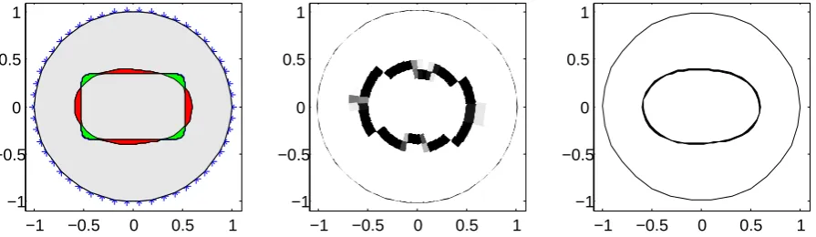
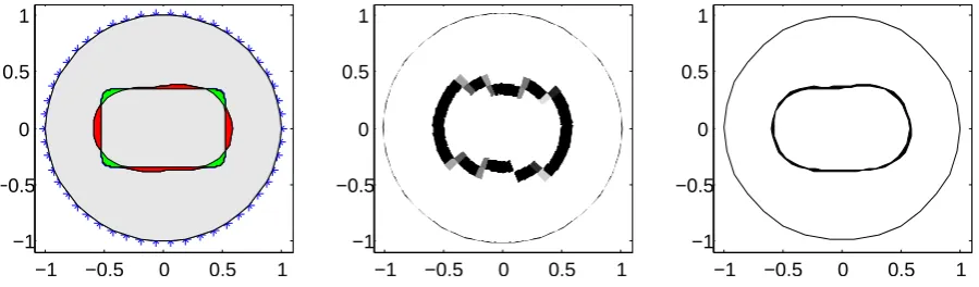
rect-angle defined in (5.3)–most numerical methods will find this problem challenging because of the relatively sharp corners to the shape. Figure 16 shows the reconstructed object and esti-mated MFS coefficients for the interface and outer boundary with prior parameters kept fixed as before. The most dramatic change is in the pattern of true MFS coefficient for the interface which is caused by the rounded corners of the rectangle. In spite of this, the reconstruction resembles the truth and the MFS coefficients for the outer boundary are well estimated. The MFS coefficient estimates for the interface however are not good, though they do following the general pattern of the interface coefficients. The posterior mean (and standard deviations) of the radii smoothing parameter is βˆr = 0.028886 (0.02519). Accuracy and variability in the object reconstruction are shown in Figure 17. The estimation errors (left) clearly show over-rounding at the corners and bulging in between – the reconstruction is too circular. The circular histogram (centre) and circular credible interval (right) indicate that variability in the posterior distribution is small.

−1 −0.5 0 0.5 1

0 2 4 6

−0.4 −0.2 0

0 2 4 6

[image:16.595.75.516.288.419.2]

−0.5 0 0.5 1

Figure 16: Round-cornered rectangular inclusion with star-shaped model with separate prior information (αr = 1.0,βc_I = 0.0116andβc_E = 0.2457): fitted shape (left) and MFS coefficients (with credible intervals) associated with the interface (centre) and outer boundary (right).

−1 −0.5 0 0.5 1

Figure 17: Round-cornered rectangular inclusion with star-shaped model with separate prior information (αr= 1.0,βc_I = 0.0116andβc_E = 0.2457): estimation errors (left), object boundary histogram (centre) and object boundary credible interval (right).

Finally, consider the full estimation, including the smoothing parameters of the MFS coeffi-cients, that is, fixing values for hyper-prior parameters αr,αcI and αcE and allowing the

esti-mation of βr,βcI and βcE in addition to the radii and MFS coefficients. Figure 18 shows the

[image:16.595.72.520.497.627.2]

(17)

rectangular object reconstruction is slightly better, with a useful improvement in the estimation of the interface MFS coefficients, and the coefficients on the outer boundary remain well esti-mated. The posterior mean estimates of the prior parameters (and standard deviations) are:

ˆ

βr= 0.0307 (0.0426),βˆc_I = 0.0322 (0.0301)andβˆc_E = 0.2331 (0.0941). Accuracy and variability in the object reconstruction are shown in Figure 19. The estimation errors (left) show a slight improvement but still the reconstruction is too circular. The circular histogram (centre) and circular credible interval (right) indicate that the posterior distribution is concentrated, hence this time allowing estimation of the prior parameters has produced a slightly more accurate reconstruction of the shape of the object. As with the bean-shape, this is also a very difficult feature to reconstruct accurately and so this estimate can be considered more than acceptable. Overall, the estimation of the round-cornered rectangular truth has been very successful.

−1 −0.5 0 0.5 1

0 2 4 6

−0.4 −0.2 0

0 2 4 6

[image:17.595.71.520.259.389.2]

−0.5 0 0.5 1

Figure 18: Round-cornered rectangular inclusion with star-shaped model with separate prior information (αr= 0.1,αc_I = 0.0001andαc_E = 0.0001): fitted shape (left) and MFS coefficients (with credible intervals) associated with the interface (centre) and outer boundary (right).

−1 −0.5 0 0.5 1

Figure 19: Round-cornered rectangular inclusion with star-shaped model with separate prior information (αr = 0.1,αc_I = 0.0001andαc_E = 0.0001): estimation errors (left), object boundary histogram (centre) and object boundary credible interval (right).

5.4 Full estimation using Laplace prior distributions

[image:17.595.70.520.466.598.2]

(18)

−1 −0.5 0 0.5 1 −1

−0.5 0 0.5 1

0 2 4 6

−0.3 −0.25 −0.2 −0.15 −0.1 −0.05 0

0 2 4 6

[image:18.595.70.518.63.199.2]

−0.5 0 0.5 1

Figure 20: Bean-shaped inclusion with star-shaped model with separate prior information (αr =

0.1,αcI = 0.0001andαcE = 0.0001) and Laplace prior distributions: fitted shape (left) and MFS

coefficients (with credible intervals) associated with the interface (centre) and outer boundary (right).

−1 −0.5 0 0.5 1

Figure 21: Bean-shaped inclusion with star-shaped model with separate prior information (αr =

0.1, αcI = 0.0001 and αcE = 0.0001) and Laplace prior distributions: estimation errors (left),

object boundary histogram (centre) and object boundary credible interval (right).

parameters,βr,βcI andβcE, as well as the MFS coefficients and the radii.

For the bean-shaped object, Figure 20 shows the reconstructed object and estimated MFS coefficients and Figure 21 shows the variability summaries. There has been little change, compared to the corresponding results using the Gaussian prior distribution (see Figures 14 and 15). However, there is a slight improvement in the accuracy of the “cusp” which reflects the Laplace distributions ability to better model abrupt changes.

[image:18.595.68.521.269.412.2]

(19)

−1 −0.5 0 0.5 1 −1

−0.5 0 0.5 1

0 2 4 6

−0.5 −0.4 −0.3 −0.2 −0.1 0 0.1

0 2 4 6

[image:19.595.73.518.136.271.2]

−0.5 0 0.5 1

Figure 22: Round-cornered rectangular inclusion with star-shaped model with separate prior information (αr = 0.1, αc_I = 0.0001and αc_E = 0.0001)and Laplace prior distributions: fitted circle (left) and MFS coefficients (with credible intervals) associated with the interface (centre) and outer boundary (right).

−1 −0.5 0 0.5 1

[image:19.595.69.519.488.625.2]

(20)

6 DISCUSSION

This paper has described the Bayesian approach to parameter estimation and the MCMC estimation algorithm, and applied them to the very practical problem of reconstructing the shape of an object from a continuous model EIT data. The MFS provides a simple yet accurate and fast approach to solving the forward problem. It is easy to describe and simple to program. However, it introduces additional, nuisance, parameters which must be estimated along with the variables of interest.

The Bayesian modelling approach gives a rigorous framework for including expert knowledge into the estimation process through prior distributions. Any beliefs regarding the nature of the parameter values, and relationships between the parameters can be incorporated. Also it provides a natural hierarchical structure to describe the dependence between variables which then allows a more intuitive description and interpretation of these relationships. Unfortunately, the prior distributions will contain additional unknown parameters. The framework also allows uncertainty in these parameters to be modelled via hyper-prior distributions. It would be pos-sible to further define hyper-hyper-prior distributions, but this usually does not add anything to the performance, nor even the flexibility, of the model.

A simple MCMC estimation algorithm was developed which allowed all parameters to be well estimated. It is important to emphasise that such algorithms must be designed with care and should be tested widely to have good confidence that they are performing well. The great bene-fit when using MCMC algorithms is that complex models can be used easily. Also, there is great flexibility in the choice of output. The posterior sample can be used to estimate any summary. For example, posterior marginal distributions can be checked for normality, and where appro-priate non-parametric techniques can be used to make inference in place of normal-based methods.

A range of simple examples have been considered and the proposed methods illustrated and developed. In the first set of examples a circular inclusion and a circular object model were used. Although of limited practical use this allowed the focus to be on the estimation of the MFS coefficients. It is clear that estimation can be improved substantially by the inclusion of prior information regarding boundary smoothing and that the two sets of MFS coefficients should be treated separately. These experiments highlight an important point that although maximum likelihood estimation is sometimes possible for such problem, and will produce a good fit to the data, it can leave parameter estimates which are not interpretable. With the inclusion of prior smoothing there is no significant deterioration in the goodness-of-fit but there is a substantial improvement in the interpretability of the MFS coefficients.

(21)

leads to a robust approach.

The results clearly indicate that the combined Bayesian/MCMC procedure has worked well, and that the MFS provides a very good and fast approximation to the forward solution. The examples have demonstrated the range of statistical models and prior distributions which can be used and the range of output summaries which are possible using MCMC sampling proce-dures. Also, the whole approach can easily be generalised making it a feasible approach even for complex modelling problems.

References

Aykroyd, R. and Cattle, B. (2006). A flexible statistical and efficient computational approach to object location applied to electrical tomography,Statistics and Computing16: 363–375.

Aykroyd, R. and Cattle, B. (2007). A flexible statistical and efficient computational approach to object location applied to electrical tomography,Inverse Problems Sci. Eng.15: 441–461.

Borman, D., Ingham, D. B., Johansson, B. T. and Lesnic, D. (2009). The method of fundamental solutions for detection of cavities in EIT,J. Integral Eqns and Appl.21: 381–404.

Brooks, S., Gelman, A., Jones, G. and Meng, X.-L. (2011). Handbook of Markov Chain Monte Carlo, Chapman & Hall/CRC.

Cowles, M. K. and Carlin, B. P. (1996). Markov chain Monte Carlo convergence diagnostics: A comparative review,J. Am. Stat. Soc.91: 883–904.

Gamerman, D. and Lopes, H. F. (2006). Markov Chain Monte Carlo: Stochastic Simulation for Bayesian Inference, 2nd edn, Chapman & Hall/CRC Texts in Statistical Science.

Gelman, A. (2006). Prior distributions for variance parameters in hierarchical models,Bayesian Analysis1: 515–533.

Gelman, A., Carlin, J. B., Stern, H. and Rubin, D. (2003). Bayesian Data Analysis, second edn, Chapman & Hall/CRC.

Geyer, C. J. (2011). Introduction to Markov Chain Monte Carlo,inS. Brooks, A. Gelman, G. L. Jones and X.-L. Meng (eds), Handbook of Markov Chain Monte Carlo, Chapman and Hall/CRC.

Haddar, H. and Kress, R. (2005). Conformal mappings and inverse boundary value problems,

Inverse Problems21: 935–953.

Ivanyshyn, O. (2007). Shape reconstruction of acoustic obstacle from the modulus of the far field pattern,Inverse Problems and Imaging1: 609–622.

(22)

Karageorghis, A., Lesnic, D. and Marin, L. (2011). The MFS for inverse geometric problems,

inL. Marin, L. Munteanu and V. Chiroiu (eds),Inverse Problems and Computational Me-chanics, Chapter 8, pp. 191–216.

Karageorghis, A., Lesnic, D. and Marin, L. (2013). A moving pseudo-boundary MFS for void detection,Numerical Methods for Partial Differential Equations29: 935–960.

Liu, J. (2008). Monte Carlo Strategies in Scientific Computing, Springer.

Raftery, A. and Lewis, S. (1995). The number of iterations, convergence diagnostics and generic Metropolis algorithms,inW. R. Gilks, S. Richardson and D. J. Spiegelhalter (eds),

Practical Markov Chain Monte Carlo, Chapman and Hall.

Roberts, G., Gelman, A. and Gilks, W. (1997). Weak convergence and optimal scaling of random walk Metropolis algorithms,Ann. Appl. Prob.7: 110–120.

Smyrlis, Y.-S. and Karageorghis, A. (2009). Efficient implementation of the mfs: The three scenarios,J. Comput. Appl. Math.227: 8392.

Stuart, A. M. (2010). Inverse problems: A Bayesian perspective,Acta Numerica19: 451–559.

Watzenig, D. and Fox, C. (2009). A review of statistical modelling and inference for electrical capacitance tomography,Meas. Sci. Technol.20: 052002 (22pp).

West, R., Aykroyd, R., Meng, S. and Williams, R. (2004). Markov chain Monte Carlo techniques and spatial-temporal modelling for medical EIT, Physiological Measurements 25: 181– 194.