This is a repository copy of Reverse glacier motion during iceberg calving and the cause of glacial earthquakes.
White Rose Research Online URL for this paper: http://eprints.whiterose.ac.uk/97243/
Version: Supplemental Material
Article:
Murray, T., Nettles, M., Selmes, N. et al. (9 more authors) (2015) Reverse glacier motion during iceberg calving and the cause of glacial earthquakes. Science, 349 (6245). pp. 305-308. ISSN 0036-8075
https://doi.org/10.1126/science.aab0460
eprints@whiterose.ac.uk https://eprints.whiterose.ac.uk/ Reuse
Unless indicated otherwise, fulltext items are protected by copyright with all rights reserved. The copyright exception in section 29 of the Copyright, Designs and Patents Act 1988 allows the making of a single copy solely for the purpose of non-commercial research or private study within the limits of fair dealing. The publisher or other rights-holder may allow further reproduction and re-use of this version - refer to the White Rose Research Online record for this item. Where records identify the publisher as the copyright holder, users can verify any specific terms of use on the publisher’s website.
Takedown
If you consider content in White Rose Research Online to be in breach of UK law, please notify us by
1 1
2
3
Supplementary Materials for
4 5
Reverse Glacier Motion During Iceberg Calving and the Cause of Glacial
6
Earthquakes
7
T. Murray, M. Nettles, N. Selmes, L. M. Cathles, J. C. Burton, T. D. James, S. Edwards, 8
I. Martin, T. OÕFarrell, R. Aspey, I. Rutt, and T. BaugŽ 9
. 10
11
correspondence to: t.murray@swansea.ac.uk 12
13 14
This PDF file includes: 15
16
Materials and Methods 17
Fig. S1 18
2 Materials and Methods
24 25
Glacial earthquake analysis 26
27
We detected glacial earthquakes by back-propagation of vertical-component seismic 28
signals recorded at stations of the global seismographic network (13, 23). We also 29
inspected back-propagated seismograms and array stacks interactively to identify 30
earthquakes too small for automatic detection by our standard algorithm (10). The 31
earthquakes were initially identified independently of image analysis; one additional 32
weak seismic signal was confirmed as an earthquake after comparison with camera 33
imagery. 34
We modelled the seismic waveforms using a centroid-single-force (CSF) formalism 35
(11, 25) to confirm earthquake locations and obtain earthquake source parameters 36
including the orientation of the force active during the earthquake, the earthquake CSF 37
amplitude, and the earthquake centroid time, tc (centroid of the temporal force history).
38
The inversion approach and data processing follow ref. 6. We assume a force-time 39
history 50 s long in which the force has a constant amplitude for one half the earthquake 40
duration, followed by a constant amplitude of opposite polarity for the remainder of the 41
duration; that is, the time function is a square wave of one cycle. The centroid time 42
corresponds to the time of the polarity reversal of the force at the earthquake half 43
duration. We note that the force-time history used in the seismic inversions is not derived 44
from the seismic data, but is prescribed. The most important feature of the time function 45
for the current analysis is the rapid change in force amplitude that occurs at tc. As
46
discussed in ref. 16, the true earthquake time function may not be symmetric, and may 47
have longer duration. Here, we choose to use the 50-s boxcar function for consistency 48
with previous systematic studies of glacial earthquakes (6, 10, 11, 13, 16). 49
We performed an experiment using the scaled force and pressure timeseries from the 50
laboratory experiments to provide input, time-varying force histories simulating a glacial 51
earthquake. The pressure timeseries were converted to a vertical force history by 52
multiplication by the map-view area of the iceberg calved, as determined from 53
photogrammetric analysis. Vertical and horizontal force histories were downsampled to 54
one sample every 10 s and modelled as a series of overlapping isosceles triangles of 55
varying height. Synthetic seismograms were calculated by summation of normal modes 56
in the preliminary reference Earth model (PREM) (26) for each triangular sub-source and 57
the seismograms summed to form the complete records. Seismograms were calculated for 58
stations at a range of distances and azimuths representative of those typically available 59
for analysis of glacial earthquakes at Helheim Glacier. The seismograms were then 60
inverted using the same approach as for data seismograms to obtain earthquake 61
parameters. 62
63
Photogrammetric analysis 64
65
Two 15.1 megapixel Canon 50D single lens reflex (dSLR) cameras were installed in 66
stereo configuration on the bedrock margins of Helheim Fjord ~4 km down-fjord (east) 67
3 hourly photographs and operated between 2013 DOY 196 and 245. Fixed 28 mm wide-69
angle lenses were used in order to capture the majority of the calving front. Digital 70
elevation models (DEMs) were produced photogrammetrically from stereo imagery using 71
the 3D visualization capabilities of SocetSET digital photogrammetry suite alongside the 72
bundle adjustment and DEM extraction components of TopconÕs ImageMaster. Ground 73
control information was extracted from a 2013 lidar DEM (27). We compared DEMs 74
prior to and following calving events to obtain three-dimensional calving geometry, 75
including the locations of the calving margins. Detailed methodology of the 76
photogrammetric processing is described in the Methods and Supplementary Material of 77
ref. 8. 78
79
Estimates of glacier thickness and iceberg aspect ratio 80
81
Estimates of glacier thickness for the DOY 206 and 212 events were made using 82
IceBridge MCoRDS L3 Gridded Ice Thickness, Surface, and Bottom, Version 2 (28). 83
Mean bottom elevations of flightline points that fell within the areal extent of each 84
calving event provided our estimates. In the vicinity of the heavily crevassed calving 85
front, errors are estimated to be ±60 m (8). 86
Iceberg aspect ratios, defined as the along-flow width of the calved iceberg to the 87
estimated iceberg height, were estimated using the photogrammetric results and an 88
equivalent rectangular iceberg, together with the estimated glacier thickness. Idealized 89
rectangular dimensions were constructed by measuring iceberg cross-glacier and along-90
flow widths and adjusting these to rectangular dimensions matching the measured map-91
view area of ice lost in each calving event. 92
93
GPS data processing 94
95
GPS sensors on ice and bedrock used Ashtech MB100 dual-frequency geodetic 96
receiver boards and ASH111661 dual-frequency antennas. 97
The position of the base station located on bedrock was estimated using the Precise 98
Point Positioning (PPP) method (29) with GIPSY-OASIS version 6.2 software from JPL. 99
In addition to base-station coordinates and a receiver clock offset, a zenith wet 100
tropospheric delay and tropospheric gradients were estimated. JPL fiducial orbit and 30-s 101
clock products were held fixed. Hydrostatic zenith delay was modelled (30) with zenith 102
delays mapped to elevation using the Global Mapping Function (GMF) (31). Ocean tide 103
loading displacements were corrected for using the FES2004 model (32) and solid Earth 104
tides were corrected according to the IERS 2010 conventions (33). Carrier-phase 105
ambiguities were fixed to integers where possible (34). 106
GPS data from sensors on the glacier surface were processed using the relative 107
carrier-phase method with TRACK version 1.29 software (35) from GAMIT 10.50. 108
Kinematic positions were estimated with respect to the fixed base station using the 109
ionosphere-free linear combination of L1 and L2 observations (LC). Baseline lengths 110
ranged from 1.5-5.6 km. An elevation-angle cutoff of 10¡ was applied. We used orbit 111
and high-rate (5 s) clock products from CODE (36). Zenith delays were modelled and 112
mapped as above (30, 31) but no wet tropospheric correction was estimated. Observations 113
4 data appended to facilitate TRACKÕs interpolation scheme. Kinematic site motion was 115
modelled using a random-walk stochastic model. The model standard deviation was set at 116
0.01 m/s0.5. Position time series were filtered to exclude data where the number of 117
unfixed biases was greater than 2, the number of double differences was fewer than 10, or 118
the height uncertainty was greater than 0.1 m. 119
120
Laboratory Experiments 121
122
Data acquisition
123 124
The laboratory experiments were performed in a fresh-water tank 244 cm long, 30 125
cm wide, and 30 cm tall, similar to tanks used previously (19, 24, 37). A model glacier 126
terminus was secured at one end of the tank. Plastic icebergs made from polyethylene 127
with a density nearly identical to glacier ice (920 kg/m3) and height HL = 20.3 cm, width
128
εHL , and cross-tank dimension DL = 26.7 cm were placed flush against the terminus and 129
allowed to capsize spontaneously under the influence of gravitational and buoyancy 130
forces. Experiments were conducted with icebergs of aspect ratio ε = 0.22, 0.28, 0.43, 131
0.54. Three levels of perforated plastic sheet were secured at an incline to the waterÕs 132
surface at the other end of the tank to damp seiche modes (38). Two different model 133
termini were used: one with an embedded pressure sensor that monitored pressure at 134
three water depths and one that was coupled to four force sensors located at each corner 135
of the terminus. The pressure and force data were acquired at a rate of 200 Hz. 136
The pressure sensor (GEMSª) had a maximum range of 2500 Pa hydrostatic 137
pressure and a response time of 5 ms. We used the pressure data recorded at the deepest 138
of the three measured depths in our analyses. The force sensors (Strain Measurement 139
Devices) each had a maximum range of 0.5 N. The sensors rely on mechanical deflection 140
to measure the force. The terminus used to measure the force was designed so that its 141
frequency response was flat in the bandwidth produced by the motion of the iceberg and 142
subsequent waves. The total force was calculated by summing the signals from all four 143
sensors and inherently represents a sum of contact and pressure forces acting on the 144
terminus. Repeat experiments showed nearly identical results for both the pressure and 145
force measurements. The results shown in Figure 3 represent the average of 3 force 146
measurements and 5 pressure measurements. The position and orientation of the plastic 147
iceberg were determined by image analysis and were used to synchronize the force and 148
pressure measurements in time. 149
150
Scaling of laboratory data
151 152
In order to compare lab data to field data, the forces and pressures measured in the 153
laboratory were scaled up to match the dimensions of icebergs at Helheim Glacier, as 154
measured by photogrammetry. Following previous studies (19, 24), the laboratory data 155
were scaled by powers of the ratio of the iceberg height in the field, HF, to the iceberg
156
height in the laboratory, HL. Because the gravitational potential energy released by
157
iceberg capsize scales as H4 (24, 39), force measurements from the laboratory were 158
scaled by (HF/HL)3, pressure measurements by (HF/HL) and time scales by (HF/HL)1/2.
159
5 field can be considered dynamically similar. The Reynolds number for flow is ~1010 in 161
the field and ~105 in the lab, but the flow is turbulent in both cases and typical drag 162
coefficients on solid bodies vary little in this flow regime (19, 24). 163
164
Prediction of glacier deflection
165 166
The scaled force and pressure are used to predict the time history of deflection of the 167
glacier-terminus region. We modeled the deflection of the calving region as an elastic 168
response to the force applied. The total force per unit area acting on the glacier terminus 169
produces a linear deflection orthogonal to the calving front such that Ftot/AF = EΔL/L,
170
where E is the YoungÕs modulus of glacial ice (~1 GPa; refs. 40, 41). The area over 171
which the total force acts is the surface area of the terminus adjacent to the capsizing 172
iceberg, AF ~ HFDF, where DF is the cross-glacier length of the calved iceberg. In Figure
173
3, the value of L was chosen so as to best match the GPS data (L=4.9 km). The length-174
scale L likely represents the approximate distance from the terminus to the grounding 175
zone. 176
The pressure reduction in the water behind the rotating iceberg creates a downward 177
force on the front of the glacier (in contrast to the upward force it causes on the solid 178
earth). The water under the ungrounded region of the glacier responds to this reduction in 179
pressure (~ 5 x 10⁴ Pa), creating a net vertical force acting on the glacier over an area AP
180
~ κLDF, where κ is the fraction of the length L over which the pressure is initially 181
reduced beneath the glacier. We model the glacier tongue as an EulerÐBernoulli beam of 182
length L with a varying load due to gravitational, buoyant, and pressure forces acting on 183
it. Our simplified model assumes the beam is clamped at the grounding line and stress 184
free at the terminus. Varying κ to match the L determined from the horizontal deflection 185
(L = 4.9 km) yields κ = 0.02, such that the pressure load is applied over a narrow region 186
parallel to the glacier terminus consistent with the dimensions of the capsizing iceberg. 187
For the comparison of predicted and observed deflection shown in Figure 3, we low-188
pass filter the scaled pressure and force traces using a 5-pole Butterworth filter with a 189
corner period of 40 s. The pressure and force records are dominated by the very-long-190
period deflection signal, and this choice of filtering does not affect our results or 191
interpretation, but serves to reduce the presence of high-frequency oscillations of the 192
water column in the tank that are expected to be damped by ice mŽlange in the glacier 193
fjord. It also removes low-amplitude, very-high-frequency sensor noise. 194
We find that the model iceberg aspect ratio for which the scaled laboratory data best 195
match the observed GPS data shown in Figure 2 is ε = 0.22, compared to a measured 196
iceberg aspect ratio from field data of 0.23. 197
6 200
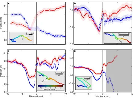
Fig. S1. 201
Additional examples of glacier response at times of glacial earthquakes. (A) Sensor 6 202
at 03:13 on DOY 206 2013; some data missing due to communications failure. (B) 203
Sensor 15 at 03:13 on DOY 206 2013. (C) Sensor 1 at 12:56 on DOY 206 2013. (D) 204
Sensor 15 at 12:56 on DOY 206 2013; sensor is lost shortly after this event. Symbols as 205
in Figure 2. Horizontal displacement for B-D has trend of 30-10 mins before tc removed
206
(B=27.6 m/day, C=27.5 m/day, D=29.4 m/day) and for panel A the trend from 10-5 mins 207
before tc (36.0 m/day). Height has mean removed. Insets (grey boxes) show plan view of
208
GPS trace during 30 minutes around tc, marked as 0; in panel (D), grey shaded region
209