Three-dimensional static and dynamic analysis of a composite cruciform structure subjected to biaxial loading: a discontinuum approach

cruciform structure subjected to biaxial loading: a discontinuum approach

.

White Rose Research Online URL for this paper:

http://eprints.whiterose.ac.uk/90590/

Version: Accepted Version

Article:

Navarro-Zafra, J., Curiel-Sosa, J.L. and Serna Moreno, M.C. (2015) Three-dimensional

static and dynamic analysis of a composite cruciform structure subjected to biaxial loading:

a discontinuum approach. Applied Composite Materials, 2015. ISSN 1573-4897

https://doi.org/10.1007/s10443-015-9453-4

eprints@whiterose.ac.uk https://eprints.whiterose.ac.uk/

Reuse

Unless indicated otherwise, fulltext items are protected by copyright with all rights reserved. The copyright exception in section 29 of the Copyright, Designs and Patents Act 1988 allows the making of a single copy solely for the purpose of non-commercial research or private study within the limits of fair dealing. The publisher or other rights-holder may allow further reproduction and re-use of this version - refer to the White Rose Research Online record for this item. Where records identify the publisher as the copyright holder, users can verify any specific terms of use on the publisher’s website.

Takedown

If you consider content in White Rose Research Online to be in breach of UK law, please notify us by

(will be inserted by the editor)

Three-dimensional static and dynamic analysis of a

composite cruciform structure subjected to biaxial

loading: a discontinuum approach

J.Navarro-Zafra · J.L. Curiel-Sosa ·

M.C Serna Moreno

Received: date / Accepted: date

Abstract A three-dimensional structural integrity analysis using the eX-tended Finite Element Method (XFEM) is considered for simulating the crack behaviour of a chopped fibre-glass-reinforced polyester (CGRP) cruciform spec-imen subjected to a quasi-static tensile biaxial loading. This is the first time this problem is accomplished for computing the stress intensity factors (SIFs) produced in the biaxially loaded area of the cruciform specimen. A static crack analysis for the calculation of the mixed-mode SIFs is carried out. SIFs are calculated for infinite plates under biaxial loading as well as for the CGRP cru-ciform specimens in order to review the possible edge effects. A ratio relating the side of the central zone of the cruciform and the crack length is proposed. Additionally, the initiation and evolution of a three-dimensional crack are suc-cessfully simulated. Specific challenges such as the 3D crack initiation, based on a principal stress criterion, and its front propagation, in perpendicular to the principal stress direction, are conveniently addressed. No initial crack lo-cation is pre-defined and an unique crack is developed. Finally, computational outputs are compared with theoretical and experimental results validating the analysis.

Keywords biaxial testing _· chopped glass-reinforced composite _· stress intensity factors·3D crack initiation and propagation

J. Navarro-Zafra

Department of Mechanical Engineering, The University of Sheffield, Sir Frederick Mappin Building, Mappin Street, S1 3JD Sheffield, United Kingdom

Tel.: +44 0014-22-7794

E-mail: jnavarrozafra1@sheffield.ac.uk J.L Curiel-Sosa

Department of Mechanical Engineering, The University of Sheffield, Sir Frederick Mappin Building, Mappin Street, S1 3JD Sheffield, United Kingdom

M.C Serna Moreno

1 Introduction

Advanced composite materials (ACM) are widely used in many industrial sec-tors such as aircraft industry, automobile industry, etc. Fundamentally, their interest is attributed to its properties: high strength-weight ratio, excellent resistant to fatigue and corrosion, satisfactory durability. However, because of the complex mechanical behaviour of these high-performance materials many experimental tests are required for designing safe components [6]. As an al-ternative for reducing the high number of experimental tests computational modelling is a remarkable approach.

Nowadays, by means of computer simulations, many phenomena of interest have already been successfully simulated e.g. car crash, a human aorta with an aneurysm, etc [15]. Nevertheless, other computational applications in the in-dustry and the scientific community remain unsolved. In computational terms, a well-known numerical method is the Finite Element Method (FEM)[3]. Most of structural integrity analyses using FEM have been based in continuum dam-age mechanics, see for instance some works applied to composites in [10] [9] [5]. This paper is proposing a discontinuous approach as explained below. When using FEM for simulating moving cracks throughout a material, several lim-itations are observed [7]. To accurate represent discontinuities with FEM it becomes necessary to conform the discretization to the discontinuity. Then, in the case of crack propagation the mesh is re-generated at each crack-growth increment with a considerable computational cost.

Over the last decades several approaches for modelling material disconti-nuities have been proposed based on the partition of unity method [14], as the GFEM [11] or the XFEM [4] developed by Belytschko and Black in 1999. In particular, XFEM permits the representation of discontinuities independently of the mesh. This characteristic makes this method able to model moving cracks with no update of the mesh during crack propagation. New develop-ments in analysis of crack growth modelling are carried out since XFEM came up [1], for instance the implementation of XFEM in 3D [22], the implementa-tion of XFEM inABAQU ST M _{[12], the delamination of GLARE [8], etc. For}

interested readers, a detail understanding of XFEM is presented in the work of Mohammadi [21].

The calculation of SIFs into the cruciform specimen are influenced by the edge effects of the specimen. A ratio relating crack size and the dimensions of the cruciform is proposed. The proposed ratio allows edge effects to be minimized with the smallest cruciform design possible. In the best authors knowledge, the SIFs calculation into a CGRP cruciform submitted to biaxial loading by means of XFEM has never been undertaken. Additionally, a 3D moving crack initiation and propagation into the structure is simulated. The crack is devel-oped as a natural outcome for all geometries based on the maximum stress criterion. Computational results are validated with experimental tests. The studied cruciform is designed for reproducing a pure biaxial loading in its central zone where shear is negligible. The CGRP composite under study be-haves in a quasi-isotropic manner. This fact is justified because of the random distribution of the fibres throughout the matrix [18],[19].

The article is organized as follows. In section 2, an introduction to XFEM is presented briefly. In section 3, the numerical model considered for repre-senting the crack behaviour of the CGRP structure is described. Section 4.1 compares computational and experimental results for three different cruciform geometries analysed under different biaxial in-plane loading cases. In Section 4.2 a static analysis of the cruciforms is completed and mixed-mode SIFs are calculated for infinite plates and the cruciform specimens under consideration. Finally, in section 5, the conclusions of the work are explained, summarizing the main achievements as a result of the research process.

2 A discontinuous approach/model based on the eXtended Finite Element Method

The general idea of the XFEM is based on including discontinuous enrichment functions to the approximation of displacements. For a 3D case, a single crack is considered (see Figure 1). The pointx∗ _{defines the crack front as depicted}

in Figure 1. It is defined also n as the normal to the crack plane. Then, the Heaviside functionH(x) takes value +1 if (x−x∗_{)·nnn≥0 and -1 otherwise,}

i.e.

H(x) =







1 if (x₋x∗_)·nnn≥0

−1 otherwise

(1)

The isotropic near-tip asymptotic functions ψj(r, θ) are included in the

displacement approximation in order to represent the asymptotic crack-tip field.

Ψ Ψ

Ψ(x) = [√rcos(θ 2),

√

rsin(θ

2),

√

rsin(θ)sin(θ

2),

√

rsin(θ)cos(θ

2)] (2)

X* X



X

X

X

1 2

3

n

Crack front

Fig. 1 Cordinate system for the crack front in 3D

uuu(e)₌

nnodes

∑

i=1

N

NNi(x)(uuui+HHH(x)aaai+

4

∑

α=1

ψ

ψψα(x)bbbαi) (3)

WhereNNNi(x) are the shape functions andnnodesnnodesnnodesthe number of nodes per

element.uuui corresponds with the nodal displacement vector used in FEM;aaai

is the nodal enriched degree of freedom vector,HHH(x) is the Heaviside function,

bbbα

i are nodal enriched degrees of freedom and ψψψα(x) the elastic asymptotic

crack-tip functions for representing the crack singularity. For the calculation of SIFs the software considers full enrichment in order to represent the dis-placement field ahead of the crack-tip. Instead, during 3D crack propagation analysis partial enrichment is considered. Particularly, the isotropic crack-tip enrichment functions are not taken into account and the only enrichment func-tion is the Heaviside funcfunc-tionHHH(x). Thus, during crack propagation the crack crosses at once a whole element without need of enriching nodes with crack-tip enrichment functions. Then, Eq.(3) becomes:

uuu=

nnodes

∑

i=1

N N

Ni(x)(uuui+HHH(x)aaai) (4)

In this work, SIFs are calculated for infinite plates and CGRP cruciforms. SIFs are extracted from the J-integral calculation [2]. This integral is a contour integral for bi-dimensional geometries and its definition in this application is extended to three-dimensional geometries. The relation between the J-integral

J and SIFs for linear elastic material [13] is given by the following equation:

J = 1

8πKKK

T_PPP−1_{KKK (5)}

whereKKK= [KI, KII, KIII]T andPPP the pre-logarithmic energy factor tensor.

Interested readers for a better understanding of fracture mechanics concepts can consult fracture mechanics references such as [2].

3 Numerical model

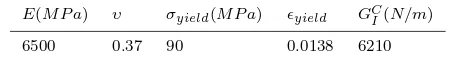
uniformly random distribution of the fibres. The material properties are de-picted in Table 1. In that table,E represents the modulus of elasticity, υthe Poisson ratio, ϵyeild the yield strain and σyield the yield strength which are

obtained in [19].

A B C

Central zone Pure biaxial stress

Fig. 2 CGRP cruciform specimens under analysis: geometry A, B and C. Notice a detailed view of geometry A in the central zone where pure biaxial loading state is observed.

Experimentally different biaxial loading cases are applied in each geometry. These loading cases cause failure through the diagonal of the central zone. 1/8 of the model for each geometry is simulated due to the symmetry. The boundary conditions applied to the three different geometries are depicted in Figure 3. Also, the cruciform specimen is fixed in the out-of-plane direction.

Fig. 3 Boundary conditions considered in the simulations for the three different cruciform geometries under biaxial loading: A,B and C.

Table 1 Material parameters

E(M P a) υ σyield(M P a) ϵyield GCI(N/m)

6500 0.37 90 0.0138 6210

4 Computational and experimental crack behaviour of the CGRP cruciform specimen

In previous work, the authors presented a two-dimensional crack initiation and propagation analysis [17]. The computational results were validated by means of comparison with experimental results. In this paper, the main objective is focused in the calculation of SIFs for the real cruciforms submitted to biaxial loading as well as quantify the edge effects into each geometry. For making that possible, previous computational tests are needed. It is important to notice that in this work a 3D model is simulated. This model has not been validated before and higher numerical complexity is expected compare with the 2D case. Therefore, in Section 4.1 crack initiation and propagation is simulated within the 3D cruciform and compared with experimental outcomes. By means of this first computational analysis the three-dimensional abilities of XFEM are demonstrated. With the confidence of this analysis, the authors are able to go further when dealing with a 3D model. In Section 4.2, a 3D static crack analysis is carried out. This section can be divided into two main parts. The first part, Section 4.2.1, considers a quasi-infinite plate subjected to biaxial loading. Those plates are equivalent to the central zone of the cruciforms and SIFs are obtained using XFEM and afterwards compared with the theoretical solution. This analysis serves to show that XFEM is capable of accurately obtain SIFs in a biaxial loading context. The second part, Section 4.2, it is focused in the calculation of SIFs within cruciform specimens once the capabilities of XFEM has been validated in previous sections.

4.1 Crack initiation and propagation

4.1.1 Constitutive Model

The constitutive model for modelling crack initiation and propagation into the cruciform is defined by means of three characteristic steps (see Figure 4) and it needs to represent the fragile fracture process of the CGRP cruciform: - Linear elastic traction-separation behaviour (point 1 to 2 in Figure 4). The elastic behaviour is defined in terms of elastic constitutive matrix that relates normal and shear stresses with nominal strains.

- Damage initiation (point 2 in Figure 4). It is connected with the begin-ning of the degradation of the cohesive response in an enriched element. The criterion of initiation selected is based on maximum principal stresses

achieve a value that it is the sum of yield stress σyield and a certain value of

toleranceσtol(define by the user) the damage process starts.

- Damage evolution (point 2 to 3 in Figure 4). Once the initiation criterion is satisfied, damage evolution defines the degradation of the stiffness (softening). The constitutive relation is written as follows σ = (1−ω)Cδ, whereω is a scalar variable that is responsible for the degradation of the stiffness. Initially this variable is zero (full load-carrying capability) and at the end of the degra-dation process this variable takes value 1 (no load-carrying capability). For a proper definition of that variable, it is requested a critical fracture energyGC

for each pure failure mode. Based on experimental observations, the dominant mode of fracture in the cruciform specimen is mode I. Then, it is assumed that the mode I of failure defines the fracture process and consequently it is defined the critical energy for pure mode I of failureGC

I. This energyGCI refers

to the energy dissipated during the damage process per unit area and its value is estimated by means of uniaxial testing. Therefore, the energy dissipated per unit volume during damage evolution isGC

I =

σyield0.01ϵyield

2 (Table 1). In this case,GC

I is equal to the critical fracture energy per unit area because the

traction-separation model considered a unitary cohesive thickness. Due to the brittle material behaviour of the composite, it is assumed that the fracture strainϵuis 1% higher than the yield strainϵyield.

Difficulties of convergence using implicit solver are detected when

strain-1



2

yield

yield



u

3

Fig. 4 Segment form by point 1 to 2: Undamaged liner elastic behaviour, point 2: damage initiation and segment form by point 2 to 3: softening.

softening behaviour is modelled. For solving this difficulty, a viscous regulariza-tion of the constitutive equaregulariza-tions defining the cohesive behaviour is adopted. In the regularization scheme a viscous damage variable is definedωv= (ω−ωv)/η,

whereη is the viscosity coefficient that represent the relaxation of time of the viscous system andω the damage variable in the inviscid model. The viscous coefficientη increments the rate of convergence of the model when it is deal-ing with strain-softendeal-ing material behaviour. Then, usdeal-ing a small coefficient (small compared with a characteristic timetc of the system) convergence can

no-Table 2 Simulation parameters

F igure Geometry Loading case σtol[P a] η[s] Initial crack

F igure5(b) A 1/2 1 10−7 _{N o}

F igure5(a) A 1/1 1 10−7 N o

F igure6(a) B 1.5/1 1 10−3 _{N o}

F igure7 C 0.5/1 1 10−3 _{N o}

ticed that one of the viscous coefficient considered during crack propagation is higher than the characteristic time of the system. However, the viscous energy involved during simulations is a 0.16 % of the total internal energy stored in the system, then, the viscous regularization does not compromise the solution and realistic results are consequently provided. It is noticed that during this research the damage tolerance σtol and viscous parameter η have a

consid-erable influence on the progression of the crack and the convergence of the solution. It is assumed that the specimen is in elastic equilibrium during the loading process so quasi-static simulations are developed employing an im-plicit solver for solving the momentum equation. An automatic time stepping is chosen. Maximum and minimum values of the time step are 10−2_{and 10}−20

respectively. 10000 increments per time step are used.

4.1.2 Validation of the 3D model by comparison with experimental tests

Crack path

(a) _(b)

Fig. 5 (a) View of the crack propagation in geometry A under loading 1/1 without definition of a priori crack (b) View of the crack propagation in geometry A under loading 1/2 without definition of a priori crack

translucent view where the surface of the crack is appreciated in the 3D ge-ometry. In Figure 6(b) it is illustrated the experimental results for geometry B under biaxial loading 1.5/1. That figure serves to illustrate the pattern of failure to achieve the correct collapse of the cruciform i.e. across the central zone. Geometry C is under a biaxial loading 0.5/1. Experimental results are accurately predicted by the simulations, therefore the computational crack is developed crossing the central zone (Figure 7).

(a) (b)

Fig. 6 (a) Computational crack propagation in geometry B under loading case 1.5/1 with-out definition of a priori crack location (b) Experimental path failure in geometry B for a biaxial loading 1.5/1 [18].

4.2 Biaxial static crack analysis

In this section, a static crack analysis is carried out into the CGRP composite. Firstly, three different quasi-infinite plates are simulated with the objective of validating XFEM for the calculation of SIFs in a biaxial contest. The size of these quasi-infinite plates is proportional to the central zone of the cruciform specimens. Secondly, SIFs are also obtain for the real cruciforms and com-pared with the analytical solution for infinite plates. A 3D model is needed for studying static crack analysis [13] within the quasi-infinite plates and the cruciform specimens. The edge effects into the SIFs calculation are studied.

4.2.1 Inclined crack in a biaxial stress field

In this section, the objective is to validate XFEM for calculating the mixed-mode SIFs in a 3D biaxial scenario. Therefore, the part of the structure with interest is the central zone of geometry A,B and C because it is where a biaxial loading is located. To study independently these regions, rectangular plates are considered for simulations (see Figure 8). The dimensions of the plates (Table 3) are one order of magnitude higher that the original central zone on the cruciforms to consider the study of an ideal quasi-infinite plate respect to the real critical area. Thus, the solution of the SIFs in mode-I and mode-II is admissible and its expression is [16]:

KIT heo=σ

√

πa(sin2β+αcos2β) (6)

KT heo II =σ

√

πa(1−α)cosβsinβ (7)

where β is the angle form by the crack and the vertical direction, σ is the stress, ais half-crack length, KT heo

I and K

T heo

II are the first and second

theoretical mode SIF, respectively.αis defined as the ratio between the major and minor stress into the plate.

As it is illustrated in Figure 8, a centre crack is defined in each plate under analysis. This crack is 2 mm long for all geometries. The crack size chosen for this analysis is relatively small compared with the dimensions of the quasi-infinite plates considered. Therefore, the quasi-quasi-infinite plate can be considered as a infinite respect to the crack size and edge effects are then minimized. The crack under analysis is inclined with an angleβ. This angle is the angle form between the crack and the vertical direction. This angle is subtracted from experiments and corresponds with the failure angle observed in the rounded zone for each geometry. The crack path is almost constant throughout the cruciform so the crack angle observed in the rounded zone is approximately the same as the central zone. Thus, for geometry A this angle is 45◦_{, for B}

33.69◦ _{and C 63.43}◦_{. The values of the load applied to the plates in each}

Table 3 Dimensions and loading in the infinite plates considered

Geometry A B C

Dimensions plate(W|H)[mm] 220x220 220x330 220x110 Loading (σx-σy)[MPa] 84-84 81.8-49.9 48-103.5

represent the width andH the hight of the plates. Thus, different values ofW

andH are considered for simulations as shows Table 3.

W

2a

H







Fig. 8 Boundary conditions of the centre crack under biaxial loading

In the neighbourhood of the crack location, it is considered a square area of 4x4 mm around a centre crack where 2500 elements are stacked in order to capture the crack-tip stress field. The major edges of the plate are partitioned into 80 equal subdivisions for each plate. The thickness of the plate is 2 mm and two mesh subdivision are considered throughout the thickness. SIFs obtain by simulations are presented in Table 3. The analytical solution is compared with the results obtained with XFEM.

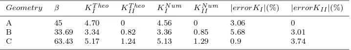
Computationally, the J-integral is considered for the SIFs calculation. It is well-known that in theory the J-integral is path independent. However, computationally this is not true. Therefore, different contours give different solutions of SIFs. In this study five contours are taken into account. Because of numerical singularities, the first contour is not considered as it is suggested in [13]. Then, the SIFs depicted on Table 4 have been obtained as the mean of the five consecutive values starting from the second value of KI andKII

calculated.

Table 4 SIFs for a 2 mm crack in the central zone of the plate

Geometry β KT heo

I KIIT heo KIN um KIIN um |errorKI|(%) |errorKII|(%)

A 45 4.70 0 4.56 0 3.06 0

B 33.69 3.34 0.82 3.36 0.85 5.68 3.01

C 63.43 5.17 1.24 5.13 1.29 0.9 3.74

mixed-mode fracture process here considered and validates its use for SIFs calculation considering a biaxial loading.

4.2.2 SIFs into the real cruciforms

In this section, SIFs are calculated for the real cruciform specimens and then compared with the theoretical solution. 1/8 of each cruciform is simulated with inclined cracks in the central zone. Different values of a i.e. half-size of the crack length, are considered,a= 0.5,1,1.5,2mm. The angle of inclination

β considered is the same as for the quasi-infinite plate analysed in previous section. Three different mesh regions can be distinguished with different ele-ment size in the structure. The first one defined is in the central zone with a 0.5 mm size, the second one defined in the arms with 1.5 mm size and the third one in the proximity of the static crack as depicted in Figure 9. For the third mesh refinement, a 4x4mm square is defined surrounding the crack with 1600 elements. The loading applied in this case is on the arms of the cruci-form. Then, for geometry A, 54M P aare applied in each arm, in geometry B,

61M P aand in geometry C, 44.25M P a. These values of load in each arm are

responsible for the final fracture of the structure. The values of SIFs obtain with the quasi-infinite plates presented on Table 4 show that the values ofKI

obtained by XFEM are higher than the ones KII. This fact is also observed

provide results close to the ones computed numerically (see Figure 12 and 13). This is justified because the length of the area loaded biaxially is not infinite if it is compared with the size of the crack

a

4 mm

4 mm

Fig. 9 Crack location in cruciform A for SIFs calculation. Note a 4x4 quadrilateral area where a special refinement is required to accurately represent the crack-tip behaviour.

In Figure 10 and 11 it is depicted the values ofKI andKIIobtained. These

values calculated by means of XFEM are represented against the half-crack size considered for each cruciform. In theory, under a biaxial loading any in-crement of the crack lengtha(maintaining all other parameters constant) will always contribute to increment the values of SIFs. This tendency is observed numerically in Figure 10 and 11. However, it is noticed a reduction in the ac-curacy of the SIF calculation when the crack size is incremented within each geometry. This is due to the edge effects that influence the SIFs calculation when using XFEM. The influence of the edge effects for the SIFs calculation depends of the size of the central zone of each geometry as shows Figure 12 and 13. In these figures, the absolute value of the relative error between theo-retical and numerical solution is presented. Higher values of error forKI and

KII are found in geometry C while geometry B is noticed a less influence of

half-crack lengthaas follows:

α= L

a = 66 (8)

According to Equation 8, for a crack size bigger than L

66 not negligible edge effects into the SIF calculation are appreciated compared with the theoretical solution. Obviously, considering a specimen with a higherα edge effects are reduced. Additionally, this analysis serves to give us a first idea of the relation between central zone and the crack size and allow future experiment tests to by oriented according to the ratio presented. It is important to notice that the values ofKI are higher thanKII in the cruciform specimens. Therefore, taken

into account the SIFs calculation with XFEM, for geometry A only mode I is observed and the shear does not exist. However, for geometry B and C it is noticed a mixed mode failure. The values of shear in geometries B and C are small compared with the normal stress. In previous studies, the shear has not been considered nevertheless here it is demonstrated computationally that it has its influence within geometry B and C.

a [mm]

0.5 1 1.5 2

K

I

[MPa m

1/2

]

0 0.5 1 1.5 2 2.5 3 3.5 4 4.5

5 A

B C

Fig. 10 KI obtained by means of XFEM is represented against the half-crack lengtha

defined for geometry A,B and C.

5 Conclusions

a [mm]

0.5 1 1.5 2

K

II

[MPa m

1/2

]

0 0.2 0.4 0.6 0.8 1 1.2 1.4

A B C

Fig. 11 KII obtained by means of XFEM is represented against the half-crack lengtha

defined for geometry A,B and C.

a [mm]

0.5 1 1.5 2

|error K

I

| [%]

0 5 10 15 20 25

30 A

B C

Fig. 12 The absolute relative error for mode-I |errorKI|(%) is represented against the

half-crack lengthafor geometries A,B and C.

a [mm]

0.5 1 1.5 2

|error K

II

| [%]

0 5 10 15 20

25 A

B C

Fig. 13 The absolute relative error for mode-II|errorKII|(%) is represented against the

half-crack lengthafor geometries A,B and C.

proposed in order to minimize edge effects and specimen size simultaneously. The dominant fracture mode into the cruciform structure is mode I according to the comparison between the numerical value ofKI andKII. In other words,

neigh-bourhood of the crack tip. In the authors best knowledge, this is the first time that SIFs are calculated for this kind of CGRP cruciform specimens. Modelling initiation and propagation was not straightforward as has been shown above and challenges that are not an issue indeed becomes critical in a 3D context, overall when dealing with fracture. The following points were addressed during this research:

- Propagation of a 3D crack front without pre-notching. - Criteria for crack initiation.

- Although re-meshing was not carried out, no deterioration of the solution was observed in terms of validation against experimental tests.

Overall, the application of XFEM here presented contributes to emphasizes that using XFEM for modelling crack in biaxial loading cases is adequate. Ad-ditionally, dealing with 3D XFEM a more realistic view of cracks is provided.

Acknowledgements This work has been financially supported by EPSRC Doctoral Train-ing Grant.

References

1. Abdelaziz, Y., Hamouine, A.: A survey of the extended finite element. Computers & Structures86(11), 1141–1151 (2008)

2. Anderson, T.L.: Fracture mechanics: fundamentals and applications. CRC press (2005) 3. Belytschko, T.: Nonlinear finite elements for continua and structures. Chichester : John

Wiley, c2000, Chichester (2000)

4. Belytschko, T., Black, T.: ELASTIC CRACK GROWTH IN FINITE ELEMENTS

620(July 1998), 601–620 (1999)

5. Carneiro Molina, A.J., Curiel-Sosa, J.L.: A multiscale finite element technique for non-linear multi-phase materials. Finite Elements in Analysis and Design94, 64–80 (2015) 6. Cox, B., Yang, Q.: In Quest of Virtual Tests for Structural Composites. Science

314(5802), 1102–1107 (2006)

7. Curiel-Sosa, J.L., Brighenti, R., Serna Moreno, M.C., Barbieri, E.: Computational tech-niques for simulation of damage and failure on composites In Beaumont P, Soutis C & Hodzic A (Ed.). Structural Integrity and Durability of Advanced Composites Woodhead Publishing (2015)

8. Curiel-Sosa, J.L., Karapurath, N.: Delamination modelling of GLARE using the ex-tended finite element method. Composites Science and Technology 72(7), 788–791 (2012)

9. Curiel-Sosa, J.L., Petrinic, N., Wiegand, J.: A three-dimensional progressive damage model for fibre-composite materials. Mechanics Research Communications35(4), 219– 221 (2008)

10. Curiel-Sosa, J.L., Phaneendra, S., Munoz, J.J.: Modelling of mixed damage on fibre reinforced composite laminates subjected to low velocity impact. International Journal of Damage Mechanics p. 1056789512446820 (2012)

11. Fries, T., Belytschko, T.: The extended/generalized finite element method: an overview of the method and its applications. International Journal for Numerical Methods in Engineering84(3), 253–304 (2010)

12. Giner, E., Sukumar, N., Taranc´on, J., Fuenmayor, F.: An Abaqus implementation of the extended finite element method. Engineering Fracture Mechanics76(3), 347–368 (2009)

14. Melenk, J.M., Babuˇska, I.: The partition of unity finite element method: basic theory and applications. Computer methods in applied mechanics and engineering139(1), 289–314 (1996)

15. Oden, J., Belytschko, T., Babuska, I., Hughes, T.: Research directions in computational mechanics. Computer Methods in Applied Mechanics and Engineering192(7-8), 913– 922 (2003)

16. Rooke, D., Cartwright, D., of Defence, G.B.M.: Compendium of stress intensity factors. London: H.M.S.O. (1976)

17. Serna Moreno, M.C., Curiel-Sosa, J.L., Navarro-Zafra, J., Mart´ınez Vicente, J.L., L´opez Cela, J.J.: Crack propagation in a chopped glass-reinforced composite under biaxial testing by means of XFEM. Composite Structures (2014)

18. Serna Moreno, M.C., L´opez Cela, J.J.: Failure envelope under biaxial tensile loading for chopped glass-reinforced polyester composites. Composites Science and Technology

72(1), 91–96 (2011)

19. Serna Moreno, M.C., Mart´ınez Vicente, J.L., L´opez Cela, J.J.: Failure strain and stress fields of a chopped glass-reinforced polyester under biaxial loading. Composite Struc-tures103, 27–33 (2013)

20. Soden, P.D., Hinton, M.J., Kaddour, A.S.: Biaxial test results for strength and defor-mation of a range of E-glass and carbon fibre reinforced composite laminates: failure exercise benchmark data. Composites Science and Technology62(12), 1489–1514 (2002) 21. (Soheil), S.M.: Extended finite element method for fracture analysis of structures.

Ox-ford : Blackwell, c2008, OxOx-ford (2008)