Theses
7-31-2019
Identifying Galaxy Mergers with Quantitative
Morphological Parameters in Simulated James
Webb Space Telescope Images
Caitlin Rose
crr9508@rit.edu
Follow this and additional works at:https://scholarworks.rit.edu/theses
This Thesis is brought to you for free and open access by RIT Scholar Works. It has been accepted for inclusion in Theses by an authorized administrator of RIT Scholar Works. For more information, please contactritscholarworks@rit.edu.
Recommended Citation
Quantitative Morphological
Parameters in Simulated James
Webb Space Telescope Images
Caitlin Rose
A Thesis Submitted in Partial Fulfillment of the
Requirements for the Degree of Master of Science in
Astrophysical Sciences & Technology
School of Physics and Astronomy
College of Science
Rochester Institute of Technology
Rochester, NY
July 31, 2019
Approved by:
Andrew Robinson, Ph.D. Date
Director, Astrophysical Sciences and Technology
Contents
1 Introduction 1
1.1 Merger Identification . . . 1
1.2 Morphology Measurements . . . 3
1.2.1 Visual Inspections . . . 3
1.2.2 Parametric Measures . . . 5
1.2.3 Nonparametric Measures . . . 8
1.2.4 High Redshift Merger Statistics . . . 18
1.3 Motivation for Current Work . . . 26
1.3.1 The Need for James Webb Space Telescope Imaging . . . 27
2 Methodology 29 2.1 Tools for Calculating Morphology Measurements . . . 29
2.1.1 The MegaMorph Project . . . 29
2.1.2 statmorph . . . 33
2.2 The SimulatedJames Webb Space Telescope Images . . . 36
2.2.1 Adding Background Noise . . . 37
2.2.2 Modifying Image Headers . . . 41
2.2.3 Resizing the Short Wavelength Images . . . 44
2.2.4 Creating Weight, Sigma, and Segmentation Maps . . . 44
2.3 The Merger History Catalog . . . 46
3 Analysis and Discussion 51 4 Conclusions 73 4.1 Summary . . . 73
Abstract
Mergers play an important role in the formation and evolution of galaxies by triggering
starbursts, AGN activity, and morphological transitions from disks to ellipticals. They
can also cause morphological disturbances in a galaxy’s appearance, such as double
nuclei, tidal tails, and other asymmetries, which can appear before or after a merger
has occurred. Therefore, one way to identify low redshift galaxy mergers is to search
for these morphological signatures via quantitative morphological parameters, which
quantify a galaxy’s light distribution (such as S´ersic profiles, or theCAS system,G and
M20, and the M ID statistics). However, for high redshift galaxies, these parameters
can be affected by biases due to poor resolution and noisy images. The upcoming
James Webb Space Telescope (JWST) will be able to probe higher redshifts than ever
before for morphological studies with high spatial resolution. The Cosmic Evolution
Early Release Science (CEERS) Survey will use JWST’s near-infrared camera to reveal
detailed galaxy morphologies over a wide range of redshifts. In preparation for CEERS
images, this works seeks to understand how well those common morphological statistics
will be able to identify JWST mergers.
Multiwavelength S´ersic profile fitting program Galapagos-2 and the
nonpara-metric morphology programstatmorphwere run on simulated JWST images from
Illus-tris, which were modified to match the specifications of CEERS imaging. Using Illustris
merger history catalogs, plots of different combinations of the rest-frame morphologies of
the simulated galaxies, binned by redshift, were made as functions of merger timescales.
These plots do not separate mergers from non-mergers as cleanly as previous studies
have found, regardless of redshift or merger timescale. This indicates that a more
so-phisticated analysis method, such as principal component analysis, will be required in
1
Introduction
1.1
Merger Identification
Mergers play an important role in the formation and evolution of galaxies – they can
cause starbursts and AGN activity when the gravitational interactions between the two
galaxies drive gas inwards from the galaxies’ disks to their centers (and the resulting
feedback can quench star formation by heating up and blowing out gas), as well as
induce morphological transitions by turning spirals into ellipticals, which occurs when
the merging process disrupts the orderly rotation of disk stars (e.g., Cox et al. 2006;
Kormendy et al. 2009). Quantifying the impact of mergers as well as how their role in
galaxy evolution has changed over cosmic time is a necessary part of understanding the
overall evolution of galaxies. However, in order to study galaxy mergers, one must first
be able to identify them in images.
There are two general methods for identifying galaxy mergers:
1. identifying close pairs (e.g., Duncan et al. 2019); and
2. identifying morphological signatures of mergers via visual classifications (e.g.,
Kar-taltepe et al. 2015) or quantitative parameters (e.g., Conselice 2003; Lotz et al.
2004; Freeman et al. 2013).
The first method finds close pairs of galaxies that have yet to merge or that are in
early phases of an interaction. This method works by selecting galaxies with projected
separations less than some chosen radius on the sky. Then true pairs are separated
from those with chance alignments along the line-of-sight by using photometric and
spectroscopic redshifts (e.g., Duncan et al. 2019).
The second method works by searching for morphological disturbances in a galaxy’s
re-cent or ongoing mergers. This project focuses on this second method and, specifically,
the quantitative tools used to characterize galaxy morphology – such as the S´ersic index
(n) andCAS, G, M20, and M IDparameters (described in Section 1.2) – some of which
have been shown to effectively locate mergers in populations of low redshift galaxies.
Section 1.2 reviews several observational and simulation papers that attempt to apply
these parameters to high redshift galaxies to better understand which parameter(s) can
effectively identify mergers in the early universe. This becomes a difficult task as redshift
increases, since image resolution, signal-to-noise, and galaxy size decrease, leading to the
loss of low surface brightness features and blurring of small scale structure. This is
il-lustrated in Figure 1, which compares the same simulated z ∼2 galaxy as seen with the
Spitzer Space Telescope (SST) and theJames Webb Space Telescope (JWST), which will
have better spatial resolution than current space telescopes (see Section 1.3.1). Clearly,
use of the SST image would result in much poorer morphological measurements than
use of the JWST image.
Figure 1: A simulated z ∼2 galaxy as seen with SST (left) and JWST (right). Source:
1.2
Morphology Measurements
1.2.1 Visual Inspections
Historically, galaxy structure has been understood through the galaxies’ visual
appear-ances. The famous “Hubble Tuning Fork,” one of the first classification systems
estab-lished by Hubble (1926, 1936) and Sandage (1961), sorted galaxies into spirals (disk
galaxies with spiral arms, gas, and young and old stars), ellipticals (smooth and round
galaxies lacking gas and young stars), lenticulars (disk galaxies lacking spiral structure,
gas, and young stars), and irregulars (galaxies that lack organized structure,
includ-ing mergers). De Vaucouleurs (1959) expanded on the Hubble Tuninclud-ing Fork to create
more elaborate spiral galaxy classifications that included bars, rings, and the degree
of tightness of the spiral arms. Van den Bergh (1960) further modified spiral galaxy
classifications to include descriptions of their bulge-to-disk ratios and van den Bergh
(1976) and Elmegreen & Elmegreen (1987) emphasized spiral arm structure in terms
of how developed or patchy the arms appear. Galaxy morphology has also been shown
to correlate with physical properties, such as mass, color, and degree of star formation
(e.g., Holmberg 1958; Roberts & Haynes 1994; Conselice 2006).
Mergers can affect these classifications by introducing features such as tidal loops
and tails, which are caused by gravitational interactions between the merging galaxies, or
double nuclei, which is when the two cores of the merging galaxies are still apparent in the
remnant. Examples of nearby interacting and merging galaxies are shown in Figure 2. In
terms of searching for mergers, visual classifications involve human classifiers inspecting
each galaxy image for these merger signatures. Visual classifications are generally robust
since the human eye is adept at picking up low surface brightness features in noisy images
(e.g., Kocevski et al. 2012; Hung et al. 2013; Kartaltepe et al. 2015).
Figure 2: Examples of nearby interacting and merging systems. Credit: NASA, ESA, the Hubble Heritage (AURA/STScI)-ESA/Hubble Collaboration, and A. Evans (University
of Virginia, Charlottesville/NRAO/Stony Brook University). Source:
http://candels-collaboration.blogspot.com/2012/09/the-role-of-mergers-in-galaxy-evolution.html
select a main morphology class, an interaction class, and various flags for each galaxy.
The main morphology class contains five options: disk, spheroid, irregular/peculiar,
compact/unresolved, and unclassifiable. The irregular/peculiar classification can
in-clude strongly disturbed objects like mergers, but not all irregular/peculiar galaxies are
mergers. The interaction class contains four options:
1. merger – single objects that appear to have undergone a merger by evidence of
tidal features/structures such as tails, loops, or double nuclei;
2. interaction within SExtractor segmentation map1– two (or more) distinct galaxies
that appear to be interacting (with clear evidence such as tidal arms, bridges, and
dual asymmetries) within one segmentation map (segmap);
1Map created bySExtractor(Bertin & Arnouts 1996) that shows where each galaxy is located and
3. interaction beyond SExtractor segmentation map – two (or more) distinct galaxies
that appear to be interacting, each with their own segmentation map; and
4. non-interacting companions – two (or more) distinct galaxies that appear near each
other on the sky, but no evidence of interactions (such as disturbed morphologies)
is present.
In Kartaltepe et al. (2015), several classifiers make visual classifications of
Hub-ble Space Telescope (HST) Cosmic Assembly Near-infrared Dark Energy Legacy Survey
(CANDELS; Grogin et al. 2011; Koekemoer et al. 2011) galaxies at z < 4. Internal
consistency tests show that the level of agreement among the classifiers depends on both
galaxy magnitude and morphology class – the fraction of objects that classifiers agree on
increases with brightness and diskiness, where disks showed the highest level of
agree-ment (>50%) while irregulars (including mergers) showed the lowest level of agreement
(< 10%). The highest levels of agreement were for the “non-interacting companions”
set and the “any interactions” set which includes the “merger,” ”interactions within
segmap,” and “interactions beyond segmap” categories. Although visual classifications
are robust, classifiers found irregulars, mergers, and interactions to be the hardest to
identify in the CANDELS sample. Additionally, classifiers had difficulty agreeing on the
specific type of interactions that merging/interacting galaxies were experiencing.
Visual classifications can be both subjective and time-consuming, especially for
large surveys. While citizen science projects (such as Galaxy Zoo; Lintott et al. 2008)
can help alleviate this problem, less subjective quantitative methods like those described
below have also been developed.
1.2.2 Parametric Measures
Galaxy structure was first quantified through the use of integrated light profiles, which
determined the mathematical form of the light profiles of elliptical galaxies while S´ersic
(1963) then generalized that to different types of galaxies:
I(r) = Ie×exp
(
−bn
"
r re
!1/n
−1
#)
, (1)
where re is the effective, or half-light, radius (the radius that contains half of the light
emitted by the galaxy), Ie is the light intensity at that radius, n is the S´ersic index,
and bn is a function of n (Graham & Driver 2005). Elliptical galaxies typically have a
de Vaucouleurs profile, where n = 4, while disks typically have an exponential profile,
where n = 1. Both re and n are used as fundamental structural parameters of galaxies
(Conselice 2014). Galaxies can also be decomposed into two-component systems: a
disk with an exponential profile and a bulge with de Vaucouleurs profile (e.g., Caon
et al. 1993; Graham & Guzm´an 2003). The bulge-to-disk (B/D) luminosity ratio is also
considered a fundamental parameter for spiral galaxies, and has been shown to decrease
from early- to late-type spirals (e.g., Graham 2001). A number of software packages
have been written to produce S´ersic fits and perform bulge-disk decompositions, such
as GALFIT (see Section 2.1.1). S´ersic index alone is unable to distinguish irregulars and
mergers from other morphological types. Irregulars, which generally lack bulges or have
weak bulges, tend to mimic disks and haven ∼1 (Tasca & White 2011; Kartaltepe et al.
2015). Therefore, studies that search for mergers using morphological signatures usually
use nonparametric measurements, which do not assume an underlying mathematical
form for the light distribution, as described in Section 1.2.3.
One possible way to use S´ersic fits to find mergers is described in Mantha et al.
(2019). They produce single S´ersic fits usingGALFITfor 17 CANDELS galaxies (z <2.5),
a simulated HST z ∼ 1.5 major2 merger, a simulated HST z ∼ 3 major merger, and
2Progenitors are two galaxies of comparable mass - typically with mass ratios >1/3 or >1/4; see
a simulated James Webb Space Telescope (JWST) z ∼ 3 major merger. By examining
GALFIT residuals (images that show the difference between the original galaxy image
and the image of the S´ersic model), Mantha et al. (2019) develop a pipeline3 to extract
residual merger signatures such as tidal tails, in addition to normal disk and spiral
substructures. For the z ∼3 major merger, Mantha et al. (2019) are unable to extract
residual features for the HST image. However, they successfully extract extended
tidal-fan features for the JWST image, which highlights JWST’s potential to better probe
high redshift mergers than HST (see Section 1.3.1 for more about the impact of JWST).
See Figure 3 for examples of their method at work.
Figure 3: Example residual structure extraction for three CANDELS galaxies: GDS
4608 (z = 1.067), GDS 14637 (z = 1.045), and GDS 14876 (z = 2.309). For each galaxy,
the original image (left), single S´ersic residual image (middle), and the extracted residual
features (solid black outlines with red shading) (right) are shown. Source: Mantha et al.
(2019)
1.2.3 Nonparametric Measures
Bershady et al. (2000), Conselice et al. (2000), and Conselice (2003) introduced
con-centration (C), asymmetry (A), and clumpiness (or smoothness) (S) in order to define
objective and quantitative measures of galaxy structure that can be used over a wide
redshift range and for many galaxy types. Together, C, A, and S comprise the CAS
system.
Concentration (C) measures how much light is in the center of a galaxy compared
to its outer regions (Bershady et al. 2000; Conselice 2003). Conselice (2003) define C as
C = 5×log10
r80%
r20%
, (2)
wherer80% and r20% are the radii of circular apertures that contain 80% and 20% of the
galaxy’s light, respectively (see Figure 4). C can range from roughly 2 to 5. Ellipticals
and spheroidal systems tend to have C >4 while disk galaxies tend to have 3< C <4.
Objects with smallC are those with low central surface brightnesses (weak bulges) and
low internal velocity dispersions (Conselice 2003). C < 0 is unphysical, and galaxies
with C < 0 may be unresolved or contaminated by point sources (Peth et al. 2016).
Asymmetry (A) measures the fraction of the galaxy’s light that is from
asymmet-ric components (Conselice et al. 2000; Conselice 2003). A is obtained by rotating the
galaxy image 180◦ around the galaxy’s center and subtracting the rotated image (I180)
from the original image (I0) and summing pixel intensities (Conselice et al. 2000) (see
Figure 4):
A =
P
|(I0−I180)|
2P
|I0|
. (3)
The center of galaxy is defined as the position that gives a minimum A value (this
center is then usually used in the determination of C and S) (Conselice et al. 2000).
which can produce asymmetric light distributions (Conselice 2003). A can range from
0 (completely symmetric) to 1 (completely asymmetric). Smooth and uniform elliptical
galaxies will have small A values (∼ 0.02), spirals generally have A ∼ 0.07 to 0.2, and
visually identified merger remnants tend to have A ∼0.3, while low surface brightness
galaxies in high background regions can have negative A values (Peth et al. 2016).
Figure 4: Graphical representation of how A, S, and C are calculated. I represents
the original image, R is the image rotated by 180◦, and B is the smoothed out image.
Source: Conselice (2003)
Clumpiness (or Smoothness) (S) measures the patchiness of a galaxy’s light
dis-tribution (Conselice 2003). First, the resolution of a galaxy image is reduced in order
to create a new image with smoothed out high spatial frequency structures. The new
smoothed image (IS) is subtracted from the original image (I0) to create a residual image
that contains only the high frequency clumps of the stellar light distribution (see Figure
4). Conselice (2003) define S as
S = 10×X(I0−IS)−B0
I0
where B0 is the background flux over an area of the sky equal to the area of the galaxy.
Galaxies with few clumpy components, such as ellipticals, will have S values near zero
while star-forming patchy galaxies, such as spirals, will have large S indices (Conselice
2003). The highly concentrated central regions are excluded from this calculation, as
are pixels with (I0−IS)<0 (Conselice 2003; Peth et al. 2016).
Conselice et al. (2000) showed that asymmetry strongly correlated with (B−V)
color for nearby galaxies undergoing normal star formation (“flocculent asymmetry”).
However, asymmetries can also be caused by dynamical events (“dynamical
asymme-try”), such as interactions and mergers which can warp disks. Merging galaxies have
dynamical asymmetries in addition to flocculent asymmetries, so their total asymmetries
deviate from the asymmetry-color sequence for normal galaxies. Therefore, Conselice
et al. (2000) find that nearby galaxy mergers are too asymmetric for their colors and
can be distinguished from other galaxy types on an asymmetry-color diagram.
Conselice (2003) extend the analysis from Conselice et al. (2000) to include 66
nearby luminous and ultraluminous infrared galaxies (LIRGs and ULIRGs), which are
very luminous galaxies that emit most of their light in the infrared and are generally
thought to be recent mergers (Sanders & Mirabel 1996). In addition to the
asymmetry-color relation, Conselice (2003) find that asymmetry also correlates with clumpiness (see
Figure 5) for nearby normal galaxies. The fit between A and S for normal galaxies is
A = (0.35±0.03)×S+ (0.02±0.01). (5)
As in Conselice et al. (2000), Conselice (2003) argue that galaxies that deviate
from the asymmetry-clumpiness relation have asymmetries caused by major mergers.
Clumpiness is less sensitive to mergers because non-interacting galaxies can still be
Figure 5: Asymmetry-clumpiness diagram for normal galaxies (solid squares) and
ULIRGs (open circles). The solid line is the relationship for normal galaxies described
with Equation 5. Source: Conselice (2003)
Figure 5 shows that the asymmetry index does not identify all ULIRGs as
merg-ers since many ULIRGs fall on the asymmetry-clumpiness relation for normal galaxies,
which means the asymmetry index is not sensitive to all phases of the merging process
(Conselice 2003). In fact, Conselice (2003) find that asymmetry only identifies galaxies
in the middle of a merger, not those in the beginning phases or those that have recently
concluded merging. Only about 50% of the URLIGs in their sample have asymmetries
that indicate the ULIRGs are ongoing major mergers. If their sample of ULIRGs
repre-sents galaxies in all phases of merging, then asymmetry underestimates the total number
of major mergers by a factor of 2.
Abraham et al. (2003) and Lotz et al. (2004) introduced the Gini coefficient (G)
and the moment of light (M20) as alternatives to the CAS system that do not assume
The Gini coefficient (G) measures the distribution of the galaxy’s light over the image
pixels. Gwas originally used in economics to describe wealth inequality in a population
(Abraham et al. 2003). Lotz et al. (2004) use a modified form of the definition ofGused
in Abraham et al. (2003):
G= 1
|X¯|n(n−1)
n
X
i
(2i−n−1)|Xi|, (6)
where n is the number of pixels and Xi is the flux value of the ith pixel.
A galaxy with a uniform light distribution (disks) will have a G around 0. A
galaxy with much of its light concentrated in a few pixels (ellipticals) will have a Gnear
1 (Peth et al. 2016). G is correlated with C, since highly concentrated galaxies will
have most of their light contained in a few central pixels, but it is independent of the
large-scale light distribution. G is different from C because G can distinguish between
galaxies with weak bulges only (which have both low C and G) and those with weak
bulges plus a few clumps of bright pixels that are not located at center (which have low
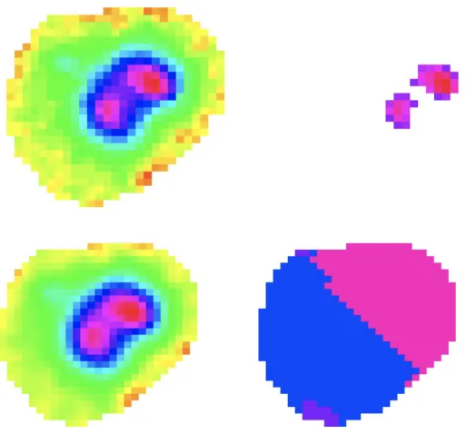
C but highG) (Lotz et al. 2004). Figure 6 shows a comparison between Gvalues andC
values for an elliptical (highly concentrated in the galaxy’s center) and a ULIRG (highly
concentrated in two regions that are not at the center).
The second-order moment of the brightest regions (M20) traces the spatial
distri-bution of bright regions such as nuclei, bars, spiral arms, and clumps of star formation
(Lotz et al. 2004). A second-order momentMi is the flux (fi) in the ith pixel multiplied
by the squared distance to the center of the galaxy (with coordinates (xc, yc)) from that
pixel (with coordinates (xi, yi)):
Mi =fi[(xi−xc)2−(yi−yc)2]. (7)
Figure 6: Comparison of C, A, S, G, and M20 values for an elliptical galaxy (top) and
a ULIRG (bottom). Source: Lotz et al. (2004)
pixels until the sum of the brightest pixels equals 20% of the galaxy’s total flux, and
then dividing by Mtot (the total second-order moment for all the galaxy’s pixels):
M20= log10
P
iMi
Mtot
, while X
i
fi <0.2ftot. (8)
M20values are usually between−0.5 and−2.5. Elliptical galaxies (with no bright
off-center clumps) will have M20 around−2.5. Disk galaxies (with star-forming clumps)
can have M20 > −1.6 (Peth et al. 2016). M20 is different from C and S because it is
weighted by the spatial distribution of bright regions (Lotz et al. 2004). Figure 6 shows a
comparison betweenM20 values for an elliptical and a ULIRG with two bright off-center
clumps.
Lotz et al. (2004) and Lotz et al. (2008) study the G− M20 relationship for
nearby galaxies and find that different types can cleanly separate in G−M20 space.
Figure 7 shows that normal galaxies fall along a definedG−M20 sequence, where early
types (E/S0/Sa) have high G and low M20 values and late types (Sb-Ir) have lower G
Figure 7: Left: G−M20 space for z = 0 galaxies from Lotz et al. (2004). Green dotted
line: divides merger candidates (ULIRGS) from normal Hubble types. Red dotted line:
divides normal early types from late types. Right: G−M20 space for HST EGS galaxies
(gray points and contours). Most galaxies lie along a well-defined sequence (solid black line). Solid green line: marks G > 3σ above the solid black line. Orange diamonds: galaxies above the dotted green line that have no visual signs of interactions. The solid contours show evidence for bimodality – the higher peak corresponds to late type
galaxies and the lower to early type galaxies. Solid red line: the minimum between the
two peaks of the bimodality. Source: Lotz et al. (2008)
galaxies. Lotz et al. (2008) adopt the following classification criteria for different types:
Mergers:G >−0.14M20+ 0.33,
E/S0/Sa: G≤ −0.14M20+ 0.33 andG > −0.14M20+ 0.8,
Sb-Ir: G≤ −0.14M20+ 0.33 andG≤ −0.14M20+ 0.8.
(9)
Snyder et al. (2015a,b) define theG−M20bulge and merger statistics. The bulge
of a galaxy along the normal galaxy sequence in G−M20 space (Snyder et al. 2015b):
F(G, M20) =
|F| G≥0.14M20+ 0.778
−|F| G <0.14M20+ 0.778
(10)
where
|F|=| −0.693M20+ 4.95G−3.85|. (11)
Bulge-dominated galaxies will have positive F values and disk-dominated galaxies will
have negative values (Snyder et al. 2015b). This statistic separates early-type and
late-type galaxies in G−M20 space.
The merger statistic (S(G, M20)) identifies galaxies that deviate from the normal
galaxy sequence – it is the distance from the diagonal line that separates low redshift
mergers and non-mergers (Snyder et al. 2015a). Rodriguez-Gomez et al. (2019) define
the merger statistic as:
S(G, M20) = 0.139M20+ 0.990G−0.327. (12)
Galaxies with negative values of S(G, M20) lie near the normal galaxy sequence and do
not have merger signatures. S(G, M20) highlights galaxies with multiple cores (large
M20) or starbursts caused by mergers (highG) (Snyder et al. 2015a).
Freeman et al. (2013) note that CAS, G, and M20 statistics become less useful
for identifying galaxies with disturbed morphologies as redshift increases and
signal-to-noise and galaxy size decreases, since small scale structure can become “washed out” as
resolution decreases (e.g., Bershady et al. 2000; Lotz et al. 2004). Therefore, Freeman
et al. (2013) introduced the M IDstatistics in order to better detect peculiar, irregular,
and merging galaxies.
Figure 8: Top: Example of pixel grouping for computing the multimode (M) statistic. The left image shows pixel intensities for a merger galaxy, while the right image shows
only those pixels associated with the largest intensity values. Bottom: Example of pixel
grouping for computing the intensity (I) statistic. The left image shows pixel intensities
for a merger galaxy, after being smoothed to remove local intensity maxima caused by noise. The right image shows pixel regions associated with each local intensity maximum
remaining after smoothing. Source: Freeman et al. (2013)
prominent regions of a galaxy (Freeman et al. 2013). First, bright regions are identified
as contiguous groups of pixels all with flux values greater than some threshold l, and
then the regions are sorted by area (Freeman et al. 2013; Peth et al. 2016). The top
images in Figure 8 show how the two largest and brightest regions have been isolated
from the rest of the galaxy. The area ratio of the two largest regions (Al,1 and Al,2) is
(Peth et al. 2016):
Rl =
Al,2
Al,1
. (13)
This calculation is repeated for different thresholds. M is then the maximum Rl value:
M is most useful for detecting double nuclei, as galaxies with double nuclei will have M
values near 1 and galaxies without will have M values near 0 (Freeman et al. 2013; Peth
et al. 2016).
Intensity (I) complements M by measuring the intensity ratio (rather than the
area ratio) between the two brightest regions in a galaxy (Freeman et al. 2013). First,
the image is smoothed with a symmetric bivariate Gaussian kernel. Then regions are
defined using maximum gradient paths, where the eight pixels surrounding each pixel are
examined and the path of maximum intensity increase is followed until a local maximum
is reached. A region consists of all pixels linked to one local maximum. The bottom
images in Figure 8 show how all of the pixels in the galaxy have been assigned to local
maxima. Then the regions are sorted by total intensity, and I is then calculated as the
ratio of intensities of the two brightest regions (I1 and I2):
I = I2
I1
. (15)
Elliptical galaxies with a bright bulge haveI values near 0 and disk galaxies with bright
clusters of star-formation will have I values approaching 1 (Peth et al. 2016).
Deviation (D) measures the distance, in pixels, from the image centroid to the
local maximum associated with I1, the brightest region found during the computation
of the I statistic (Freeman et al. 2013). Since apparent distances are larger for closer
galaxies, the distance used for D is normalized by an approximate radius, pnseg/π,
where nseg is the number of pixels associated with the galaxy:
D=
r π
nseg
p
(xcen−xI1)
2−(y
cen−yI1)
2. (16)
Here (xcen, ycen) and (xI1, yI1) mark the coordinates of the image centroid and brightest
D is designed to measure asymmetry and is complementary toA (Freeman et al.
2013). For spheroidal and disk galaxies (even disk galaxies with defined spirals or bars),
D should tend towards 0, while galaxies with bright star-forming regions at large
dis-tances from the galaxy center should have higher D values (Freeman et al. 2013; Peth
et al. 2016). Freeman et al. (2013) demonstrate that D and A are not redundant by
computingDandAfor a sample of high redshift galaxies and concluding that, although
there is some correlation between the two, D can capture evidence of asymmetry that
A misses, and vice-versa.
Freeman et al. (2013) calculateM IDstatistics for galaxies in the HST GOODS-S
field for which visual classifications andCAS,G, andM20 measurements were available.
They study the relative importance of each of the CAS, G, M20, and M ID statistics
for detecting peculiar/irregular (“non-regular”) galaxies and mergers (see Figure 4 in
Freeman et al. 2013), and conclude that I is the most important statistic for detecting
both non-regulars and mergers and that M is better than D for detecting mergers but
D is better thanM for detecting non-regulars. Freeman et al. (2013) also conclude that
M ID plusA are the most important statistics for detecting non-regulars and mergers –
those four measures together are just as effective at identifying mergers as the full set of
CAS, G, M20, and M ID. Figure 9 shows the four-dimensional space of the M ID and
A statistics for the HST galaxies in their sample.
1.2.4 High Redshift Merger Statistics
At high redshifts, characterizing morphology and identifying high redshift merger
can-didates can be difficult due in part to poor spatial resolution and loss of low surface
brightness features (such as tidal tails). How well do the quantitative measures
de-scribed above identify mergers at high redshifts (z >1)? This section reviews a number
Figure 9: Scatter plots of theM IDand Astatistics for HST GOODS-S galaxies. Green circles: visually-identified mergers. Blue crosses: visually-identified irregulars that are
not mergers. Red lines: density of regular galaxies. Black lines: best-fitting linear
regression functions. For clarity, only 100 randomly selected non-regulars/mergers are
shown. Source: Freeman et al. (2013)
In addition to introducingGand M20, Lotz et al. (2004) also study morphologies
of Lyman-break galaxies in the HST Deep Field North (1.7 < z < 3.8) using CAS, G,
and M20. Lotz et al. (2004) expect that the poor spatial resolution of higher redshift
galaxies will bias their observed morphologies, so they simulate mean biases in each
of the quantitative measurements by degrading their images of low redshift galaxies to
mimic observations of higher z galaxies. Lotz et al. (2004) find that the uncertainties
introduced to A and S make them ineffective at distinguishing between spheroidal and
disk galaxies. C and M20 also have biases that depend on morphological type, but they
are more useful than A and S. G was the least biased diagnostic out to z∼3.
Figure 10 showsC−AandG−M20 plots for the observed Lyman-break galaxies
Figure 10: Left panels: C−AandG−M20plots of HDF-N Lyman-break galaxies (open
squares: LBGs with spectroscopic redshifts; filled squares: LBGs with photometric
redshifts) as well as for low redshfit galaxies degraded to higher z resolutions (symbols
the same as for the right-hand panels). Right panels: C−AandG−M20plots for normal
low redshfit galaxies (circles: E/S0; triangles: Sa–Sbc; crosses: Sc–Sd; diamonds: dI).
Source: Lotz et al. (2004)
2004). Lotz et al. (2004) find that the biases in the quantitative measurements cause the
Lyman-break morphologies to appear similar to low redshift early-type morphologies,
although some of the Lyman-break galaxies have higher G and A than expected. They
determine, through a series of tests between the Lyman-break galaxy morphologies and
the degraded low redshift galaxy morphologies, that the Lyman-break galaxies are
actu-ally unlikely to have morphologies similar to low redshift ellipticals and spirals (<0.4%
probability). The high G and A values imply they are more similar in morphology to
low redshift ULIRGs.
Conselice et al. (2008) compares visual classifications of HST UDF galaxies (z ∼
3) to theirCAS, G,andM20values. Figure 11 shows the concentration-asymmetry plane
Figure 11: C − A plane for different redshift bins. Solid black lines: separates the regions populated by different galaxy types for nearby galaxies. The colors correspond
to visual classifications. Open blue circles: peculiar galaxies (including mergers). Solid
red squares: ellipticals, S0s, and compact galaxies. Cyan triangles: ellipticals with
minor peculiarities (such as asymmetries in outer regions or dual nuclei). Green crosses:
face-on disk galaxies. Green dots + solid lines: edge-on disks. Source: Conselice et al.
(2008)
bins, 86±10% of the galaxies found in the merger space of Figure 11 (where A >0.35)
were in fact classified by eye as a peculiar/merger. However, only 20±3% of the total
number of galaxies classified as peculiars actually fell within the merger region. So
although C −A was generally successful at isolating mergers from other types, it also
failed to identify all of the mergers (Conselice et al. 2008). This true for all redshift bins.
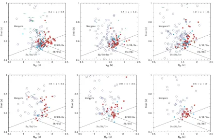
Figure 12 shows theG−M20plane for different redshift bins for the same sample
of galaxies. At 0.4 < z < 0.8, 75±10% of visually-identified peculiar galaxies fall in
Figure 12: G−M20 plane for different redshift bins. Solid black lines: separates the
regions populated by different galaxy types for nearby galaxies from Lotz et al. (2008).
The colors correspond to visual classifications as in Figure 11. Source: Conselice et al.
(2008)
were peculiars. In this case, G−M20 identifies a higher fraction of peculiar galaxies as
mergers thanC−A, but also mis-identifies a higher number of non-peculiars as mergers
than C−A (Conselice et al. 2008). Again, this is true for all redshift bins.
Conselice et al. (2008) conclude that visual classifications generally agree with
positions in CAS and G− M20 spaces. G −M20 identifies more visual peculiars as
mergers, but also has more contamination by non-peculiars falling into G−M20 merger
space. This implies that eitherG−M20 is not locating true mergers or that G−M20 is
more sensitive to merger timescales than CAS.
Peth et al. (2016) use principal component analysis (PCA) of C, A, G, M20, and
the seven different (yet related) morphology parameters into fewer variables (principal
components) to reduce redundancy and find the natural distributions of data in the new
parameter space. The three most important principal components (PCs) that Peth et al.
(2016) define are:
1. PC1 (bulge strength) – galaxies with low PC1 values have high S´ersic indices and
high F (recall Equations 10 and 11) which are indicative of strong bulges, while
higher PC1 values correlate with smaller bulges and more dominant disks;
2. PC2 (concentration dominance) – galaxies with large PC2 tend to have bright
centers and extended envelopes; and
3. PC3 (asymmetry dominance) – galaxies with large PC3 tend to be more
morpho-logically disturbed.
Using their PCA results, Peth et al. (2016) sort their galaxies into nine
morpho-logical groups using a hierarchical clustering method. Figure 13 shows G−M20 space
for each of these groups (for plots of the other morphological parameters, see Figures 7
- 11 in Peth et al. 2016).
Peth et al. (2016) find that Group 9 galaxies are asymmetric/irregular and have
strong bulge components. They lie along theG−M20dividing line between mergers and
non-mergers. They have moderate values for C (∼ 3.7±0.7), G (∼ 0.52±0.05), M20
(∼ −1.40±0.27), andM ID (∼0.14±0.14, ∼0.21±0.18, ∼0.19±0.09, respectively),
and high values for A (∼ 0.21±0.10). Galaxies in this group are the most visually
disturbed out of all the groups – visual classifications from Kartaltepe et al. (2015)
indicate that nearly 24% of Group 9 galaxies are irregular, while disks, spheroids, and
disk + spheroids make up only 41%, 13%, and 11% of Group 9, respectively. Peth
et al. (2016) find that Group 9 galaxies display tidal features and otherwise irregular
Figure 13: G−M20 space for each group. Dotted lines: divide mergers (top left corner)
from bulge-dominated galaxies (right-most region) and disk-dominated galaxies (bot-tom left region), modified from Lotz et al. (2004). The panels are roughly arranged by PC1 (increasing left to right) and PC2 (increasing bottom to top). Star-forming
galax-ies are denoted by stars and quenched galaxies by circles. Group -1 are outliers that
don’t fit into the other groups, likely because they have poorly measured morphological
parameters. Source: Peth et al. (2016)
Group 0 consists of galaxies with strong bulge components and faint smooth
extended components that populate the spheroidal region of theG−M20diagram. Group
6 is the largest group (37% of the entire sample), with the highest fraction of quenched
galaxies (43%), and are characterized by compact sizes and smooth features. TheG−M20
diagram in Figure 13 classifies them as borderline disk/spheroidal. Peth et al. (2016)
find that Groups 6, 9, and 0 have a evolutionary connection. Initially, galaxies belong to
Group 6 where they are simple bulges with no surrounding structure. They would then
transition to Group 9 galaxies after gas-rich mergers induce star formation and create
disturbed features like tidal tails. After star formation fades and gas settles into disk or
Thompson et al. (2015) use simulated HST CANDELS galaxies (2 < z < 4)
created with GADGET-3to study C, A, G,andM20. First, Thompson et al. (2015) define
a merger ratio R as the ratio of the masses of the two merging galaxies and define
major mergers to have mass ratios > 1 : 4. Then Thompson et al. (2015) find that
asymmetry (A) most strongly correlates with merger ratio when compared to any of the
other parameters (see Figures 5 - 13 in Thompson et al. 2015). Thompson et al. (2015)
examine A in more detail (see Figure 16 in Thompson et al. 2015), and find that the
typical asymmetry merger threshold ofA >0.35 does not perform significantly better at
identifying mergers than no threshold value (A >0) for any time or for any orientation.
Increasing A thresholds does improve the ability of A to correctly identify mergers.
While A > 0.35 can only correctly identify mergers ∼ 10% of the time, A > 0.8 can
correctly identify mergers∼ 50% of the time andA >1.5 can correctly identify mergers
∼ 70% of the time. However, while increased Athresholds can improve the accuracy of
merger detections, it can also diminish the ability of A to identify a complete sample
of mergers (higher A thresholds will overlook more mergers). Additionally, A performs
slightly better for edge-on orientations and for pre-coalescence timescales. Thompson
et al. (2015) conclude that A performs better than the other quantitative statistics for
detecting high z mergers. Furthermore, high asymmetry thresholds (such as A > 0.8)
work better than the typical A > 0.35 cut used for low redshift galaxies, at the risk of
sacrificing a more complete sample set of mergers.
Snyder et al. (2015a) use hydrodynamic simulations of HST images (1 < z <3)
with ARTto study C, A, G, M20, and M ID. They study the evolution of a single galaxy
from z ∼ 3 to z ∼ 1, as viewed from five different camera angles, that experiences a
major merger attmerge = 0 (which corresponds toz = 1.6) (see Figure 11 in Snyder et al.
2015a), and find that G, M20, and M ID are sensitive to different stages of the merger
(t < tmerge) while M ID statistics are activated for an extended period of time after
coalescence att =tmerge. The decrease in theG−M20 merger statistic after coalescence
implies that the merger signatures are being obscured by the galaxy’s global structural
evolution. The galaxy is becoming more centrally concentrated, so it is evolving inM20
such that the G−M20 merger statistic is lowered (recall Equation 12) which leads to
a false negative (even though this galaxy is a recent merger). Therefore, Snyder et al.
(2015a) conclude that the ability to identify a merger with G−M20 depends on the
galaxy’s overall initial or evolving structure, which can hide signs of a recent merger.
Snyder et al. (2015a) also study the evolution of a galaxy that experiences a minor
merger around t = 6 Gyr which triggers a disk-wide starburst event (see their Figure
14). Following the minor merger, the galaxy has enhanced M ID but not an enhanced
G−M20 merger statistic. In this case, the galaxy is disk-dominated so it has a low G
value which lowers the G−M20 merger statistic. Again, Snyder et al. (2015a) find that
G−M20 merger statistic is affected by the galaxy’s overall morphology. Additionally,
M ID is also enhanced during non-merger events where the disk happens to contain
bright clumps of star formation (t ∼ 5 Gyr). Therefore, they conclude that sometimes
M ID can falsely identify clumpy, growing disks as mergers.
1.3
Motivation for Current Work
Many studies have analyzed the ability of common morphological statistics to identify
mergers at high redshifts, where morphological statistics can be affected by biases caused
by poor resolution and noisy images. Lotz et al. (2004) find that among CAS, G, and
M20, G is the least biased statistic out to z ∼ 3 and that high G and A identify a
population of high z galaxies similar to low redshift ULIRG mergers. Conselice et al.
(2008) find that among CAS, G, and M20, G−M20 correctly identify more visually
CAS system atz ∼3. They note thatG−M20 may be more sensitive to merger phase
than CAS parameters. Peth et al. (2016) use the more sophisticated PCA method
to group galaxies according to morphology for redshifts of 1.4 < z < 2. They find
that Group 9 galaxies with strong asymmetries and bulges tend to be visually classified
irregulars/mergers. Thompson et al. (2015) study simulated galaxies at 2 < z < 4 and
find that simply using higher asymmetry cuts (A >0.8) correctly identifies more mergers
thanC, G,orM20, although higher asymmetry cuts also overlook many less asymmetrical
mergers. Additionally, they find thatAis slightly biased towards edge-on orientations as
well as merger phase. Finally, Snyder et al. (2015a) study simulated 1 < z <3 galaxies
and find that Gand M20 andM ID are sensitive to merger phase, whereGand M20are
enhanced prior to coalescence and M IDare enhanced post-coalescence. G andM20 are
sensitive to the galaxy’s overall structure which can obscure merger signatures. M ID
can also be enhanced for non-merging clumpy galaxies. G and M20 and M ID can also
change depending on orientation.
These studies show that identifying mergers using quantitative measurements can
be quite complicated. Attempting to correctly identify a larger fraction of true mergers
comes with the price of contaminating the true merger sample with non-mergers.
Ap-plying harsher criteria rids merger samples of contaminants but also misses less obvious
true mergers. Additionally, quantitative measurements can also overlook true mergers
or incorrectly identify non-mergers due to effects like galaxy orientation, overall
struc-ture, and merger phase. Therefore, one must be careful to understand exactly what each
parameter is sensitive to in order to build complete samples of true mergers.
1.3.1 The Need for James Webb Space Telescope Imaging
While astronomers have no control over orientations or merger timescales of observed
im-prove image quality and resolution for higher redshift galaxies. JWST is the highly
an-ticipated successor to the Hubble Space Telescope (HST). The Cosmic Evolution Early
Release Science (CEERS) Survey is a survey designed to demonstrate the capabilities
of JWST by utilizing JWST imaging and spectroscopy in parallel over 100 arcmin2 on
the HST EGS field for galaxies in a large redshift range of 0.5 < z < 13 (Finkelstein
et al. 2017). CEERS will address both core extragalactic JWST science drivers: “First
Light and Reionization” and “The Assembly of Galaxies.” Under the “The Assembly of
Galaxies” goal, CEERS imaging will be used to understand the morphologies of early
galaxies and track their size and structural evolution. CEERS will use JWST’s near
in-frared camera (NIRCam) to probe higher redshifts than HST (out to redshift z ∼7 for
morphological studies) with high spatial resolution to reveal galaxies with both regular
and irregular/perturbed morphologies, star-forming and quiescent galaxies, and mergers
in great detail. High quality imaging will also prompt a reexamination of z <4 galaxies.
At the time of writing, JWST is scheduled to launch by March 30, 20214.
The studies discussed above show how astronomers can find different quantitative
parameters to be useful for locating mergers, depending on their datasets and specific
objectives. Therefore, a comprehensive analysis of these statistics as applied to simulated
JWST galaxies is necessary to define and test a robust method for specifically identifying
JWST mergers. This should be done before the first images are available to allow for
quick and efficient analysis of JWST mergers once JWST images become available.
For my project, I will use simulated JWST images, modified to meet the
specifi-cations of CEERS, in order to evaluate the ability of these quantitative measurements
to identify high redshift JWST galaxy mergers. Future work will focus on designing and
testing the framework for effectively locating JWST mergers in anticipation of CEERS
observations.
2
Methodology
Section 2.1 describes the programs used to make quantitative morphological
measure-ments on galaxies in the simulated JWST images, which are described in Section 2.2.
Many of the modifications made to the simulated images were motivated by the
require-ments of these programs.
2.1
Tools for Calculating Morphology Measurements
2.1.1 The MegaMorph Project
TheMegaMorphProject5 is a project designed to improve astronomers’ ability to measure
the structure of galaxies via parametric methods (i.e., S´ersic fits) while making full
use of modern multiwavelength imaging surveys (Bamford et al. 2011; H¨außler et al.
2013; Vika et al. 2013). Using multiwavelength information allows one to constrain fit
parameters to vary smoothly as a function of wavelength, which produces more physically
consistent models. For example, a normal disk galaxy’s blue, exponential disk will be
more prominent in bluer bands and its red, de Vaucouleurs bulge will be more prominent
in redder bands; therefore it should have a low S´ersic index in blue bands with smoothly
increasing S´ersic indices toward redder bands (H¨außler et al. 2013). Color gradients
within stellar populations and dust attenuation can also cause different S´ersic indices as
a function of wavelength (H¨außler et al. 2013). Therefore, fixing the light profile shape
as a function of wavelength would result in poor fits in other bands, while allowing it
to vary freely can result in wildly different fit parameters between the bands (H¨außler
et al. 2013). Simultaneous multiband profile fits with the fit parameters constrained to
vary smoothly with wavelength preserves the different structural components and allows
for physically meaningful color gradients (Bamford et al. 2011; H¨außler et al. 2013; Vika
1000 1500 2000 2500 3000 3500 4000 4500
[nm]
0.85 0.90 0.95 1.00 1.05 1.10 1.15
n
F115W F150W F200W F277W F356W F444W
(a)Galapagos-2ID: 828
1000 1500 2000 2500 3000 3500 4000 4500 [nm]
0 1 2 3 4 5 6
n F115W F150W F200W F277W F356W F444W
(b)Galapagos-2ID: 940
Figure 14: Left: S´ersic indices for Galapagos-2 ID: 828 (Figure 15a), which are ∼ 1
for all bands. Right: S´ersic indices for Galapagos-2ID: 940 (Figure 15b), which range
from ∼0 to ∼6.
et al. 2013). See Figure 14 for examples of how S´ersic indices can vary with wavelength.
Under the MegaMorph Project, Galapagos6 (Barden et al. 2012) was modified to create
Galapagos-2 and Galfit7 (Peng et al. 2002, 2010) was modified to create GalfitM.
Galfit is a least-squares fitting algorithm that uses a Levenberg-Marquardt
al-gorithm to find the optimum solution to the S´ersic fit for a galaxy (Peng et al. 2002,
2010; Peng 2012). Galfit finds the best fit solution by minimizingχ2
ν (the reducedχ2),
an indicator of the goodness of fit. Galfit calculates χ2ν via (Peng 2012):
χ2ν = 1
NDOF nx
X
x=1
ny
X
y=1
(fdata(x, y)−fmodel(x, y))2
σ(x, y)2 , (17)
where NDOF is the degree of freedom (the number of pixels minus the number of free
parameters), fdata(x, y) is the input science image, fmodel(x, y) is the model generated
byGalfit, andσ(x, y) is the sigma image (see Section 2.2.4). Galfitcan only accept a
single input image soGalfit’s modelfmodel(x, y) is not wavelength-dependent. GalfitM
6https://borishaeussler.github.io/galapagos v1/home.html
can accept several input images, each a different band, in order to perform simultaneous
multiband fitting (H¨außler et al. 2013). GalfitM’s model is a wavelength-dependent
function (H¨außler et al. 2013):
M(x, y;p1, . . . , pn)→M[x, y; ˜p1(λ;q1,1, . . . , q1,m1), . . . ,p˜n(λ;qn,1, . . . , qn,mn)], (18)
where pi are the model parameters of original Galfit and each ˜pi is a function, with
parameters qi,j, that describes how model parameter i varies with wavelength λ for
GalfitM. The model parameters are position (x, y), magnitude, half-light radius, S´ersic
index, axis ratio and position angle (which describes the orientation of the galaxy’s
semi-major axis with respect to the y-axis of the image). BothGalfitand GalfitMcan
perform single S´ersic fits and two-component S´ersic fits for bulge-disk decomposition.
Galapagos(Galaxy Analysis over Large Areas: Parameter Assessment byGalfit
-ting Objects fromSExtractor) is essentially anIDLwrapper routine that allowsGalfit
to be used for large survey images, since Galfit can only be run on one galaxy at a
time (Barden et al. 2012). Galapagos reads in a large survey image, usesSExtractor8
(Source Extractor; Bertin & Arnouts 1996) to detect the objects in the field, cuts out
postage stamps of each detected galaxy, prepares input files forGalfit, instructsGalfit
to perform the actual fits for each of those galaxies, and compiles the final catalog with
the S´ersic fits for all galaxies. Galapagos-2 performs the same function as Galapagos,
but Galapagos-2 can read in multiple large survey images for different bands and calls
to GalfitMfor multiband fitting (H¨außler et al. 2013).
SExtractorworks by detecting objects via thresholding (Bertin & Arnouts 1996;
Holwerda 2005). In order for an object to be detected, the object’s pixels must be
above some specified threshold (e.g., have a value greater than three times the estimated
background value) and be adjacent to each other, and there also must be more adjacent
pixels than a specified minimum number. During this procedure, SExtractor must
also decide whether a group of pixels above the threshold level is a single object or
several close objects (such as in the case of merging galaxies). To do this, SExtractor
examines the light distribution within the group of pixels and constructs a “tree” (see
Figure 2 of Bertin & Arnouts 1996) that shows which pixel subgroups (“branches”)
have an integrated intensity greater than some fraction of the total intensity of the
entire pixel group. If there are two or more branches, then each branch is considered a
separate object. SExtractor assigns the remaining pixels to the objects by computing
the probability for each pixel to belong to each of the separate objects.
This deblending technique does become less efficient for faint or poorly resolved
galaxies (Bertin & Arnouts 1996). Therefore SExtractor can either properly deblend
brighter objects while failing to detect faint objects or it can detect faint objects while
improperly splitting up bright and clumpy galaxies (Barden et al. 2012). To overcome
this, Galapagos (and Galapagos-2) runs SExtractor twice – once in “cold” mode
for proper deblending and once in “hot” mode for faint object detection – where the
SExtractor setup files required by Galapagos/Galapagos-2 which have thresholding
and deblending parameters that emphasize the two different modes (Barden et al. 2012).
Then Galapagos/Galapagos-2creates the list of detected objects for Galfit/GalfitM
by discarding any hot objects that are too close to cold objects (duplicates), and adding
the remaining hot objects to the cold catalog. Galapagos-2 only calls SExtractor on
one band, and uses the catalog from this detection image to cut out stamps and write
setup files for all bands for GalfitM (H¨außler et al. 2013).
In addition to the final output catalog with the S´ersic fit parameters,Galapagos-2
also outputs the original stamp, the GalfitM model, and the residual image for each
0 50 100 150 200 0 25 50 75 100 125 150
0 50 100 150 200 0 25 50 75 100 125 150
0 50 100 150 200 0 25 50 75 100 125 150
(a) Right: Input F200W image stamp, Middle: GalfitM single S´ersic model, Left: Residual image forGalapagos-2ID: 828. This galaxy had S´ersic indices∼1 for all bands (Figure 14a). The axes are in pixels. X-axis is 217 pixels (13.6700) and y-axis is 169 pixels (10.6500).
0 50 100 150 200 250 300 0 50 100 150 200 250
0 50 100 150 200 250 300 0 50 100 150 200 250
0 50 100 150 200 250 300 0 50 100 150 200 250
(b) Right: Input F200W image stamp, Middle: GalfitM single S´ersic model, Left: Residual image forGalapagos-2ID: 940. This galaxy had S´ersic indices ranging from∼0 (F115W) to
∼6 (F277W) (Figure 14b). X-axis is 295 pixels (18.5900) and y-axis is 335 pixels (21.1100).
Figure 15: Examples of Galapagos-2 output stamps for simulated JWST galaxies (see
Section 2.2).
2.1.2 statmorph
statmorph9 is a PYTHON package for calculating nonparametric morphology
measure-ments, including all the measurements discussed in Section 1.2.3, as well as single S´ersic
fits (Rodriguez-Gomez et al. 2019). statmorph can handle both single galaxy images
or survey images, but it cannot handle multiple images at once to make full use of
multiwavelength imaging. Instead, each filter has to be run independently. statmorph
requires:
1. the background-subtracted image containing the galaxy or galaxies of interest;
2. a corresponding map that shows where each galaxy is located (a segmentation
map; see Section 2.2.4); and
3. a multiplicative factor that converts the image into units of electrons.
For every source labeled in the segmentation map, basic shape and size
mea-surements are calculated such as the centroid (xc, yc), which later serves as an initial
guess for the galactic center that minimizes the asymmetry index; the half-light radius
rhalf, which is the radius that contains half of the light emitted by the galaxy; and the
petrosian radiusrpetro, which is the radius at which the mean surface brightness is equal
to some fraction (typically 0.2) of the mean surface brightness within that radius. Then
statmorph calculates the mean, median, and standard deviation of the background by
drawing a “skybox” on a region near the galaxy of interest that contains only background
pixels according to the segmentation map. The skybox is also used during calculations of
the asymmetry (A) and smoothness (S) indices to measure the asymmetry and
smooth-ness of the sky. The nonparametric measures are calculated using the same definitions
as in Section 1.2.3, although Rodriguez-Gomez et al. (2019) do rename the clumpiness
index to the smoothness index S (but the definition and abbreviation do not change).
Finally, a S´ersic profile is fit to each galaxy using the astropy.modeling10 package.
Fitting is done using the Levenberg–Marquardt algorithm, like Galfit, and the initial
guesses for the fit parameters are based on the nonparametric measurements.
Figure 16 illustrates some example statmorph measurements. The black circles
in the Gini Segmap images enclose the pixels used for G and M20 calculations and the
colored regions in theWatershed Segmapimages indicate the pixels associated with each
local brightness maximum for theI statistic (similarly tobottom of Figure 8). The blank
regions in the Original Image,Original Segmap, andGini Segmap images in Figure 16b
indicate the presence of nearby galaxies that were masked out.
flag = 0 Ellip. (Centroid) = 0.1751 Ellip. (Asym.) = 0.1728
Original Image (Log Stretch)
Centroid Major Axis (Centroid) Asym. Center Major Axis (Asym.) Half-Light Ellipse
flag_sersic = 0 Ellip. (Sérsic) = 0.2333 n = 1.6273
Sérsic Model + Noise
Sérsic Center Major Axis (Sérsic) Half-Light Ellipse (Sérsic)
Sérsic Residual, I Imodel Asymmetry Residual, I I180
Sky Mean = 0.0054 Sky Median = 0.0055 Sky Sigma = 0.0087
Original Segmap
Skybox
S/N = 7.6892
G = 0.5587 M20= 1.9628
F(G, M20) = 0.1658
S(G, M20) = 0.0467
C = 3.2254A = 0.0180 S = 0.0260
Gini Segmap
M = 0.0075 I = 0.0282 D = 0.0137
Watershed Segmap (I statistic)
First Peak
Second Peak AS= 0.3077
Shape Asymmetry Segmap
Asym. Center
rpetro, circ rpetro, ellip rmax
(a) Examplestatmorph measurements forstatmorph ID: 1601.
flag = 0 Ellip. (Centroid) = 0.2229 Ellip. (Asym.) = 0.2231
Original Image (Log Stretch)
Centroid Major Axis (Centroid) Asym. Center Major Axis (Asym.) Half-Light Ellipse
flag_sersic = 0 Ellip. (Sérsic) = 0.3185 n = 0.5908
Sérsic Model + Noise
Sérsic Center Major Axis (Sérsic) Half-Light Ellipse (Sérsic)
Sérsic Residual, I Imodel Asymmetry Residual, I I180
Sky Mean = 0.0024 Sky Median = 0.0022 Sky Sigma = 0.0077
Original Segmap
Skybox
S/N = 45.3543
G = 0.4379 M20= 1.2735
F(G, M20) = 0.9101
S(G, M20) = 0.0705
C = 2.2173 A = 0.3853 S = 0.0530
Gini Segmap
M = 0.8298 I = 0.5360 D = 0.0170
Watershed Segmap (I statistic)
First Peak
Second Peak AS= 0.3772
Shape Asymmetry Segmap
Asym. Center
rpetro, circ rpetro, ellip rmax
[image:39.612.82.532.110.583.2](b) Example statmorphmeasurements forstatmorph ID: 939.
Figure 16: Examples of F277W statmorph measurements for simulated JWST galaxies
2.2
The Simulated
James Webb Space Telescope
Images
The simulated JWST images11 used in this project were created by Snyder et al. (2017)
and are drawn from the Illustris Simulations12 (Nelson et al. 2015; Vogelsberger et al.
2014). The Illustris Project is a series of hydrodynamical simulations of galaxy formation
in a cube that is 106.5 Mpc on a side. Illustris incorporates models for cooling, star
formation, stellar evolution and stellar feedback, gas recycling, metal enrichment, and
supermassive black hole growth and AGN feedback (Nelson et al. 2015; Vogelsberger
et al. 2014). Illustris has been shown to reproduce the observed stellar mass function,
the SFR-mass main sequence, and the Tully-Fisher relation for z < 3 (Torrey et al.
2014) as well as the observed merger rate for z <1 (Rodriguez-Gomez et al. 2015).
Snyder et al. (2017) use Illustris-1, the highest resolution simulation. To create
the simulated images, Snyder et al. (2017) use the lightcone technique of Kitzbichler &
White (2007) to create mock images that mimic the geometry of current deep galaxy
surveys while preserving large-scale structure. Snyder et al. (2017) choose two integers
(n, m) to set the origin of their lightcone (or the position of a virtual observer, at
z = 0) and define the viewing direction from the origin with the unit vector ˆu3 =
(n, m, nm)/|(n, m, nm)|. Along the line traced out by ˆu3, Snyder et al. (2017) fill each
volume segment of the lightcone with Illustris output from earlier and earlier cosmic
times. Snyder et al. (2017) choose (n, m) = (11,10) to produce a “thin” lightcone that
subtends a unique volume from z = 0 to z = 18 over an area of ∼ 8 square arcmin.
This default lightcone is used to create the “Field B” simulated image. Snyder et al.
(2017) then swap the x and y coordinates of Field B to create Field A, and the x and
z coordinates to create Field C. The three fields will not necessarily contain unique
galaxies, but the 3D structure will be different between the three perspectives.
For this project, I use the original Field B images in the same infrared filters that
will be observed by the CEERS program (F115W, F150W, F200W, F277W, F356W,
and F444W) (Finkelstein et al. 2017). Each filter has its own fits file which contains the
following extensions:
1. IMAGE NOPSF - Raw image without PSF or noise;
2. SimulationAssumptions - URL links to Illustris documentation and API;
3. MockDataAssumptions - Contains code and parameter choices for creating mock
images;
4. IMAGE PSF - Raw image convolved with model PSF from WebbPSF;
5. MODELPSF - The PSF model;
6. Catalog - Lightcone Catalog, containing intrinsic simulation information, including
galaxy ID numbers and Illustris snapshot numbers, image positions, redshifts, star
formation rates, masses, etc.; and
7. CatalogDocumentation - Strings containing explainers of catalog columns.
Information about each of the six filters used in this project are listed in Table 1.
Much of the information relating to NIRCam and its filters were taken from the online
JWST user documentation (“JDox”) (Space Telescope Science Institute 2016). All filters
have an AB magnitude zeropoint of 31.40 as listed in the headers of the simulated images
(Snyder et al. 2017).
2.2.1 Adding Background Noise
The extensions labeled IMAGE PSF provide the mock images that have already been
Table 1: Filter parameters.
Channel Filter Pivot λa PHOTFLAMb Pixel Scalec Gaind Read Noised
µm erg/cm2/˚A/e− 00/pix e−/ADU e−
F115W 1.154 2.251∗10−22 0.031 2.05 16.2
Short λ F150W 1.501 1.331∗10−22 0.031 2.05 16.2
F200W 1.989 7.577∗10−23 0.031 2.05 16.2
F277W 2.762 3.929∗10−23 0.063 1.82 13.5
Long λ F356W 3.568 2.355∗10−23 0.063 1.82 13.5
F444W 4.408 1.543∗10−23 0.063 1.82 13.5
ahttps://jwst-docs.stsci.edu/display/JTI/NIRCam+Point+Spread+Functions bSee Section 2.2.2
chttps://jwst-docs.stsci.edu/display/JTI/NIRCam+Overview
dhttps://jwst-docs.stsci.edu/display/JTI/NIRCam+Detector+Performance
background noise that real survey images would have, nor do they correlate with any
specific exposure time. Therefore, I needed to add noise that corresponds to the CEERS
exposure time.
Pandeia13 is the JWST exposure time calculator (ETC) developed to aid
as-tronomers in writing JWST proposals (Pontoppidan et al. 2016). For a given filter,
source, and detector setup, Pandeia will generate a small postage stamp (or “scene”)
of the desired source (such as a point source or an extended galaxy) and calculate the
signal-to-noise for that scene for the given exposure time (Pontoppidan et al. 2016). The
maximum field of view of the scene is 1000. Instructing the source to be offset from the
center of the scene by more than 1000 will result in a scene that is purely background
noise. Pandeia’s background accounts for various components that will contribute to
JWST backgrounds – zodiacal and Milky Way light, stray light from objects outside
the field of view, and thermal emission from the telescope itself – and includes noise
due to the MULTIACCUM readout pattern, inter-pixel capacitance, and cosmic rays
(Pontoppidan et al. 2016). The scene can then be downloaded from Pandeia as a fits
file, along with any of Pandeia’s calculations for the scene. I used Pandeiato generate
0.32 0.34 0.36 0.38 0.40 0.42 0.44 0.46
Pixel value
0 5 10 15 20 25 30
Normalized number
= 0.39
[image:43.612.128.489.83.350.2]Gaussian distribution F277W original noise
Figure 17: Gaussian distribution (orange line) overlaid on a histogram of all pixel values
from the PandeiaF277W noise image.
noise images for each filter corresponding to the exposure time listed in the CEERS
proposal: 2866.72 seconds from 3 exposures of 5 groups each in DEEP8 readout mode,
at the coordinates of the HST EGS field (Finkelstein et al. 2017).
The background scenes downloaded from Pandeiaare small – only ∼300 pixels
on each side – while the simulated images are much larger – 5378 pixels on a side for
the short wavelength images and 2631 pixels on a side for the long wavelength images.
Therefore, larger noise images were created by drawing from a Gaussian distribution
with the mean and standard deviation of the Pandeia images but with the size of the
simulated images using numpy.random.normal14. As seen in Figure 17, the noise of
the Pandeia images can be approximated very well by a Gaussian distribution. As an
example, the background noise image for the F277W filter is shown in Figure 18a.
The units of the simulated images were originally nanoJy and were converted to
0 500 1000 1500 2000 2500 0
500 1000 1500 2000 2500
(a) Background noise
0 500 1000 1500 2000 2500
0 500 1000 1500 2000 2500
[image:44.612.94.521.83.305.2](b) Background-subtracted noisy image
Figure 18: Background noise and background-subtracted noisy image for the full-size
F277W image. The axes are in pixels. Both images are 2631 pixels (2.760) on a side.
counts sec−1 using thePHOTFNUkeyword already present in the headers of the simulated
images, which gives the flux in Jy at 1 count sec−1. ThePandeianoise images (and
there-fore the Gaussian noise images) were originally in electrons sec−1 and were converted
to counts sec−1 using the GAIN keyword (see Table 1) that was added to the headers
(see Section 2.2.2). Then the Gaussian noise images were simply added to the simulated
images. This is a similar procedure to that of Rodriguez-Gomez et al. (2019), who added
Gaussian background noise to their Illustris images in order to comparestatmorph
out-put between Illustris images and real survey images from the Pan-STARRS1