Mon. Not. R. Astron. Soc.345,1145–1186 (2003)
Dynamo processes and activity cycles of the active stars AB Doradus,
LQ Hydrae and HR 1099
J.-F. Donati,
1A. Collier Cameron,
2M. Semel,
3G. A. J. Hussain,
2P. Petit,
1B. D. Carter,
4S. C. Marsden,
1,4M. Mengel,
4A. L´opez Ariste,
3,5S. V. Jeffers
2and D. E. Rees
61Laboratoire d’Astrophysique, Observatoire Midi-Pyr´en´ees, F-31400 Toulouse, France 2School of Physics and Astronomy, University of St Andrews, St Andrews KY16 9SS 3LESIA, Observatoire de Paris-Meudon, F-92195 Meudon-Cedex, France
4Faculty of Sciences, The University of Southern Queensland, Toowoomba 4350, Australia 5High Altitude Observatory–NCAR, PO Box 3000, Boulder, CO 80307, USA
6CSIRO Division of Radiophysics, PO Box 76, Epping, NSW 2121, Australia
Accepted 2003 July 18. Received 2003 July 3; in original form 2002 September 27
A B S T R A C T
In this paper, we present new brightness and magnetic surface images of the young K0 dwarfs AB Doradus and LQ Hydrae, and of the K1 subgiant of the RS CVn system HR 1099 (=V711 Tauri), reconstructed from Zeeman–Doppler imaging spectropolarimetric observations col-lected at the Anglo-Australian Telescope during five observing campaigns (totalling 50 nights), from 1998 January to 2002 January. Along with the older images of the same stars (published in previous papers), our complete data set represents the first long-term series on temporal fluctuations of magnetic topologies of very active stars.
All of the magnetic images presented here indicate that large regions with predominantly azimuthal magnetic fields are continuously present at the surfaces of these stars. We take this as further evidence that the underlying dynamo processes that produce them are probably distributed throughout the entire convective zone (and not confined at its base, as in the Sun). We speculate that the radial and azimuthal field maps that we recover correspond, respectively, to the poloidal and toroidal components of the large-scale dynamo field.
We find, in particular, that some signatures, for instance the relative fraction of magnetic energy stored in the large-scale poloidal and toroidal field components, and the polarity of the axisymmetric component of the field, are variable with time, and provide potentially fruitful diagnostics for investigating magnetic cycles in active stars other than the Sun. We report here the detection of partial polarity switches in some of the axisymmetric field components of two of our programme stars (AB Dor and LQ Hya), suggesting that the dynamo operating in these stars may be cyclic.
Key words:line: profiles – stars: activity – binaries: close – stars: magnetic fields – stars: rotation – stars: spots.
1 I N T R O D U C T I O N
Zeeman–Doppler imaging or ZDI (Semel 1989; Brown et al. 1991; Donati & Brown 1997) is an innovative tomographic method simi-lar to Doppler imaging (e.g. Vogt, Penrod & Hatzes 1987) that can
E-mail: [email protected] (J-FD); [email protected] (ACC);
[email protected] (MS); [email protected] (GAJH); [email protected] (PP); [email protected] (BDC); [email protected] (SCM); [email protected] (MM); [email protected] (ALA); svj1@st-andrews. ac.uk (SVJ); [email protected] (DER)
reconstruct images of the surface magnetic field of rapidly rotating cool active stars, from high-resolution phase-resolved spectropo-larimetric observations. As opposed to all other techniques for in-vestigating stellar magnetic fields (e.g. Borra & Landstreet 1980; Robinson 1980; Basri, Marcy & Valenti 1992), which only yield magnetic field parameters averaged over the visible stellar disc (or at least over the visible magnetic regions), ZDI can recover both the location and the shape of magnetic regions at the surface of rapidly rotating cool active stars, but also (to a certain extent) the orienta-tion of field lines within these magnetic regions. In this respect, ZDI represents a very promising opportunity to study the surface mag-netic field structures of cool stars other than the Sun, as well as their
temporal evolution (magnetic cycles) and the underlying dynamo processes, in a manner very similar to that used in the particular case of the Sun (e.g. Stenflo 1992).
ZDI has now been successfully applied to active stars of various evolutionary status, ranging from pre-main sequence to red giant branch stage. Magnetic fields have been detected in approximately 25 stars (e.g. Donati et al. 1997), and mapped for six of them (e.g. Donati et al. 1992, 1999; Donati & Cameron 1997; Donati 1999). The extremely surprising result obtained in these studies is that all such stars feature magnetic regions in which the field is mainly azimuthal, i.e. parallel to the surface and oriented along lines of equal latitude. At first order, the polarity of these azimuthal field regions is independent of longitude, suggesting that they actually reflect the toroidal component of an axisymmetric large-scale dynamo field and that the underlying dynamo processes operate within the bulk of the convective zone (rather than being confined to the interface with the radiative interior as in the Sun).
Monitoring such magnetic structures has already revealed signif-icant long-term evolution possibly attributable to magnetic cycles (Donati 1999). For instance, the field structure of the K1 subgiant of the RS CVn system HR 1099 (=V711 Tauri) has evolved from an almost purely azimuthal field topology at epoch 1990.9 to a mixed field distribution at following epochs, indicating that the underlying activity cycle is probably in the phase of regenerating the poloidal component of the large-scale dynamo field. Similarly, the appear-ance, at the surface of the young K0 dwarf LQ Hydrae at epoch 1996.99, of a high-latitude azimuthal field feature with a polarity opposite to those detected in all previous maps may suggest that this star has recently undergone a new global polarity switch.
In this paper, we present new spectropolarimetric observations of the young ultrafast rotator AB Dor, of the young K0 dwarf LQ Hya and of the evolved K1 subgiant of the RS CVn system HR 1099, obtained during five major campaigns at the Anglo-Australian Tele-scope (AAT) with Semel’s visitor polarimeter and the UCL echelle spectrograph (UCLES), taking place in 1998 January, 1998 De-cember and 1999 January, 2000 DeDe-cember, 2000 DeDe-cember, 2001 December and 2002 January, and corresponding to a total number of 50 allocated nights. From these observations (detailed in Section 2), we reconstruct new maximum entropy brightness and magnetic sur-face images (presented in Sections 3–5) for all three stars and five epochs, thus expanding the time series already published by Donati et al. (1992), Donati & Cameron (1997), Donati (1999) and Donati et al. (1999). Finally we briefly discuss in Section 6 some of the implications of these new results for our knowledge of large-scale field structures and dynamo processes in cool active stars.
2 O B S E RVAT I O N S A N D M O D E L L I N G T O O L S
2.1 Instrumental setup
The observational setup used for this new series of observation is very similar to that described in Donati et al. (1997, 1999), Donati & Cameron (1997) and Donati (1999). It consists of a visitor polarime-ter mounted at the Cassegrain focus of the 3.9-m Anglo-Australian Telescope, and collecting stellar light through a 1.8-arcsec circular aperture. Note that the polarimeter used for these runs is completely new and now involves, in particular, quarter-wave and half-wave Fresnel rhombs (e.g. Bennett 1970) to achieve a very achromatic po-larimetric analysis. We no longer rotate the quarter-wave retarder, as in the previous setup (e.g. Donati et al. 1997), because of the lateral beam displacement it generates (as a single Fresnel paral-lelepiped), but rotate instead the half-wave Fresnel rhomb (made of
two optically contacted Fresnel parallelepipeds inducing no lateral beam displacement, and placed after the quarter-wave rhomb in the beam) with the same overall result as in the old setup (an exchange of both beams throughout the whole instrument). A double optical fibre then conveys the light from the polarimeter down to the UCL echelle spectrograph, fed through a Bowen–Walraven image slicer device (set in a two slice per fibre configuration). The refocusing optics attendant to the image slicer were the same as those described in Donati et al. (1999), yielding a total slit size of 3.8×0.45 mm2at
the entrance of the spectrograph, except in 1999 December where the old 1995 December slicer setup was used (see table 1 in Donati et al. 1997).
The other significant change with respect to the set up described in Donati et al. (1999) concerns the CCD detector. In the first four ob-serving seasons reported here, we used a MIT/LL CCD with 2048× 4096 15µm2pixel, while an EEV CCD with the same format, but
smaller (13.5µm2) pixels, was made available to us in the last run.
As both chips are larger than the unvignetted field of UCLES cam-era, we used a smaller window format (2048×2448 pixel for the MIT/LL chip and 2048×2746 pixel for the EEV chip) to reduce read-out time (down to approximately 1 min in fast mode). With the 31.6 groove mm−1 grating, up to 52 orders (number 80–131) can
be fully recorded on to the MIT/LL detector, ensuring full spectral coverage from 430 to 715 nm in a single exposure with significant overlap (as much as a half free spectral range for the bluest orders) between successive orders. For the EEV chip, the full spectral cov-erage is slightly smaller (46 orders altogether, ranging from number 84 to 129 and covering from 437 to 681 nm), but this loss of pho-tons is largely compensated by the much higher quantum efficiency of the CCD in most of the spectral window (up to a factor of 2 at 430 nm and a factor of 1.5 at 500 nm). Note that the reduced detector window format ensures that vignetting within the UCLES camera should only be, for each order, approximately 10 per cent larger on both order edges than at the order centre.
With the MIT/LL (respectively, EEV) detector, the slit (convolved with the spectrograph broadening profile) projects on to 29×2.5 pixel (respectively, 33×2.7 pixel), yielding an average spectral resolution of approximately 70 000 and an average pixel size of
Figure 1. Resolving power of UCLES as a function of the order of number, when using either the EEV (full line) or the MIT/LL chip (dashed line), the 31.6 groove mm−1grating and a 0.45 mm wide slit. The resolution in each order is estimated from the average full width at half maximum of approximately 40 Th lines.
Dynamo processes and activity cycles
1147
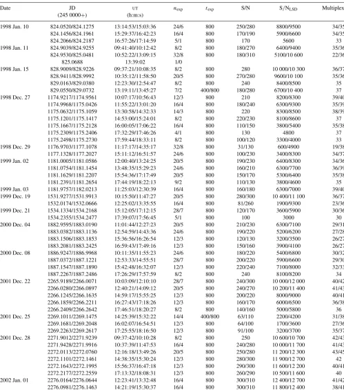
Table 1. Journal of observations for AB Dor. The first column lists the date of observation, while columns 2 and 3 indicate the Julian date and Universal Time of the first and last subexposure of each continuous series. Column 4 mentions the total number of individual subexposures/polarization sequences in the associated series of subexposures. Columns 5–8 indicate, for each polarization spectrum, the corresponding total exposure time, peak S/N ratio per pixel (of 1.9 km s−1for the first four runs, and of 1.7 km s−1 for the fifth one), S/N ratio in the associated StokesVleast-squares deconvolved spectra (per 2
km s−1velocity bin for the first four runs, and per 1.7 km s−1bin in the fifth one), and multiplex gain in S/N ratio, respectively. Note that whenever more
than one polarization sequence is available in a continuous series (i.e. for most AB Dor observations), these columns list the range of variations of these parameters.
Date JD UT nexp texp S/N S/NLSD Multiplex gain
(245 0000+) (h:m:s)
1998 Jan. 10 824.0520/824.1275 13:14:53/15:03:36 24/6 800 250/280 8800/9500 34/35
824.1456/824.1961 15:29:37/16:42:23 16/4 800 170/190 5900/6600 34/35
824.2066/824.2187 16:57:26/17:14:59 5/1 800 170 5600 33
1998 Jan. 11 824.9039/824.9255 09:41:40/10:12:42 8/2 800 180/270 6400/9400 35/36
824.9530/825.0481 10:52:22/13:09:15 32/8 800 180/310 5100/10 600 22/36
825.0688 13:39:02 1/0
1998 Jan. 15 828.9009/828.9226 09:37:21/10:08:35 8/2 800 280 10 000/10 300 36/37
828.9411/828.9992 10:35:12/11:58:50 20/5 800 270/280 9600/10 100 35/36
829.0163/829.0380 12:23:30/12:54:47 8/2 800 240 8400/8500 35
829.0550/829.0732 13:19:11/13:45:27 7/2 400/800 180/280 6700/10 400 37
1998 Dec. 27 1174.9217/1174.9561 10:07:17/10:56:43 12/3 800 210 8200/8300 39/40
1174.9968/1175.0426 11:55:22/13:01:20 16/4 800 180/240 6300/9300 35/39
1175.0632/1175.1059 13:30:58/14:32:33 14/3 800 220 8300/8500 38/39
1175.1201/1175.1417 14:53:00/15:24:01 8/2 800 220/230 8100/8600 37
1175.1667/1175.2128 16:00:05/17:06:22 16/4 800 110/150 3800/5400 35/38
1175.2309/1175.2406 17:32:29/17:46:26 4/1 800 130 4800 37
1175.2498/1175.2730 17:59:44/18:33:11 8/2 800 100/120 3300/4000 33
1998 Dec. 29 1176.9703/1177.1078 11:17:17/14:35:17 32/8 800 31/130 600/4900 19/38
1177.1328/1177.2027 15:11:12/16:51:57 24/6 800 100/230 3400/8300 34/37
1999 Jan. 02 1181.0005/1181.0586 12:00:40/13:24:25 20/5 800 190/230 6400/8300 34/36
1181.0754/1181.1454 13:48:35/15:29:23 24/6 800 160/210 6300/7700 36/39
1181.1629/1181.2207 15:54:36/17:17:49 20/5 800 150/170 5300/6400 35/38
1181.2391/1181.2654 17:44:19/18:22:13 9/2 800 110/130 3800/4600 35
1999 Jan. 03 1181.9757/1182.0213 11:25:03/12:30:39 16/4 800 160/180 6300/7000 39/40
1999 Dec. 19 1531.9277/1531.9913 10:15:50/11:47:27 20/5 800 280/300 10 400/11 100 36/37
1532.0174/1532.0666 12:25:02/13:35:55 16/4 800 81/260 1900/9300 23/36
1999 Dec. 21 1534.1334/1534.2168 15:12:05/17:12:15 28/7 800 120/170 3600/5900 30/36
1534.2355/1534.2477 17:39:07/17:56:45 5/1 800 100 3000 30
2000 Dec. 04 1882.9595/1883.0190 11:01:44/12:27:23 20/5 800 210/230 6300/7100 29/31
1883.0382/1883.1136 12:54:59/14:43:36 24/6 800 190/220 5200/6200 27/28
1883.1506/1883.1853 15:36:56/16:26:54 12/3 800 120/130 3200/3500 26/27
1883.2081/1883.2425 16:59:43/17:49:16 12/3 800 150/160 3900/4100 26/27
2000 Dec. 08 1886.9247/1886.9968 10:11:35/11:55:23 24/6 800 180/220 5400/6800 30/32
1887.0372/1887.1221 12:53:33/14:55:51 28/7 800 200/220 5900/6600 29/30
1887.1547/1887.1890 15:42:48/16:32:07 12/3 800 220/240 7100/8000 32/33
1887.2267/1887.2486 17:26:29/17:57:59 8/2 800 240 8100/8200 34
2001 Dec. 22 2265.9189/2266.0071 10:03:09/12:10:10 28/7 800 240/300 10 000/12 000 40/42
2266.0280/2266.0897 12:40:21/14:09:12 20/5 800 240/270 10 200/11 400 41/43
2266.1245/2266.1635 14:59:17/15:55:25 12/3 800 200/220 8000/9000 40/41
2266.1859/2266.2211 16:27:43/17:18:26 12/3 800 160/170 6000/6500 36/38
2266.2409/2266.2642 17:46:51/18:20:27 8/2 800 140/160 5000/5800 36
2001 Dec. 25 2269.1011/2269.1475 14:25:39/15:32:22 14/4 400/800 63/110 2200/4200 31/38
2269.1681/2269.2048 16:02:07/16:54:51 12/3 800 64/100 1700/3600 27/36
2269.2263/2269.2617 17:25:55/18:16:50 12/3 800 91/100 3200/3700 35/37
2001 Dec. 28 2271.9012/2271.9239 09:37:42/10:10:28 8/2 800 250 10 600/10 700 42/43
2271.9428/2271.9916 10:37:39/11:47:53 16/4 800 240/280 10 000/11 700 41/43
2272.0113/2272.0760 12:16:18/13:49:26 20/5 800 250/280 11 200/12 300 43/45
2272.1101/2272.1461 14:38:35/15:30:24 12/3 800 280/300 11 900/12 700 42
2272.1643/2272.1995 15:56:37/16:47:18 12/3 800 290/300 11 600/12 200 40/41
2272.2177/2272.2559 17:13:32/18:08:31 12/3 800 260/290 10 500/11 600 40
2002 Jan. 01 2276.0164/2276.0644 12:23:41/13:32:48 16/4 800 300/310 12 400/12 700 41/42
2276.0981/2276.1463 14:21:19/15:30:37 16/4 800 300/310 11 800/12 400 38/41
2276.1656/2276.1880 15:58:25/16:30:39 8/2 800 290/300 11 900/12 200 41
Table 2. Same as Table 1 for LQ Hya.
Date JD UT nexp texp S/N S/NLSD Multiplex gain
(245 0000+) (h:m:s)
1998 Jan. 10 824.0240/824.0368 12:34:37/12:52:57 4/1 1200 170 5900 35
824.2253/824.2421 17:24:24/17:48:37 5/1 1200 100 3300 33
1998 Jan. 11 825.1914/825.2047 16:35:40/16:54:48 4/1 1200 130 4600 35
1998 Jan. 12 826.0367/826.0497 12:52:51/13:11:38 4/1 1200 140 4800 34
826.0956/826.1082 14:17:39/14:35:48 4/1 1200 110 3900 35
826.2231/826.2359 17:21:13/17:39:46 4/1 1200 100 2500 25
1998 Jan. 15 829.0032/829.0124 12:04:35/12:17:50 4/1 800 110 4400 40
829.1751/829.1842 16:12:05/16:25:18 4/1 800 130 4900 38
1998 Dec. 27 1175.1457/1175.1549 15:29:51/15:43:00 4/1 800 130 4600 35
1998 Dec. 28 1176.0798/1176.0925 13:54:53/14:13:12 4/1 1200 29 800 28
1176.1018/1176.1145 14:26:35/14:44:52 4/1 1200 73 1700 23
1176.1537/1176.1663 15:41:16/15:59:29 4/1 1200 67 2000 30
1998 Dec. 29 1177.0472/1177.0578 13:07:54/13:23:11 4/1 970 36 900 25
1177.2073/1177.2199 16:58:35/17:16:43 4/1 1200 120 4300 36
1998 Dec. 30 1178.0425/1178.0552 13:01:15/13:19:25 4/1 1200 88 2800 32
1178.1281/1178.1408 15:04:31/15:22:43 4/1 1200 110 4000 36
1178.2000/1178.2129 16:47:59/17:06:31 4/1 1200 73 2100 29
1178.2535/1178.2577 18:05:01/18:11:07 2/1 600 30 800 27
1999 Jan. 02 1181.1495/1181.1587 15:35:21/15:48:30 4/1 800 120 4400 37
1999 Jan. 03 1182.0878/1182.0969 14:06:23/14:19:32 4/1 800 110 4200 38
1182.1398/1182.1489 15:21:20/15:34:29 4/1 800 120 4300 36
1182.2049/1182.2141 16:55:04/17:08:16 4/1 800 130 4600 35
1999 Dec. 20 1533.0693/1533.0824 13:39:49/13:58:42 4/1 1200 110 3600 33
1533.1694/1533.1819 16:03:52/16:22:00 4/1 1200 140 4700 34
1533.2561/1533.2688 18:08:43/18:27:03 4/1 1200 120 4100 34
1999 Dec. 21 1534.0979/1534.1105 14:21:00/14:39:11 5/1 1200 160 5500 34
1999 Dec. 29 1542.0600/1542.0726 13:26:26/13:44:34 4/1 1200 170 5300 31
1542.2012/1542.2139 16:49:46/17:07:59 4/1 1200 220 8100 37
2000 Dec. 04 1883.1189/1883.1317 14:51:12/15:09:43 4/1 1200 100 2700 27
1883.1904/1883.2033 16:34:10/16:52:45 4/1 1200 89 2600 29
1883.2475/1883.2604 17:56:28/18:15:00 4/1 1200 130 4200 32
2000 Dec. 05 1884.1334/1884.1463 15:12:10/15:30:41 4/1 1200 170 5300 31
1884.2016/1884.2149 16:50:22/17:09:24 4/1 1200 130 4400 34
1884.2576/1884.2670 18:10:58/18:24:29 4/1 800 100 3500 35
2000 Dec. 06 1885.1266/1885.1419 15:02:15/15:24:17 4/1 800 100 3200 32
1885.2028/1885.2121 16:51:59/17:05:29 4/1 800 150 5100 34
2000 Dec. 07 1886.1502/1886.1630 15:36:13/15:54:41 4/1 1200 75 1900 25
1886.2463/1886.2557 17:54:44/18:08:14 4/1 800 50 1000 20
2000 Dec. 08 1887.1262/1887.1358 15:01:42/15:15:36 4/1 800 120 4000 33
1887.1937/1887.2031 16:39:00/16:52:28 4/1 800 160 5100 32
1887.2534/1887.2628 18:04:52/18:18:22 4/1 800 170 5500 32
2000 Dec. 09 1888.1143/1888.1237 14:44:33/14:58:04 4/1 800 74 2200 30
1888.1782/1888.1877 16:16:39/16:30:14 4/1 800 74 2100 28
1888.2415/1888.2510 17:47:45/18:01:30 4/1 800 100 3100 31
2000 Dec. 10 1889.1123/1889.1217 14:41:39/14:55:11 4/1 800 110 3700 34
1889.1760/1889.1854 16:13:26/16:27:01 4/1 800 130 4600 35
1889.2469/1889.2594 17:55:30/18:13:33 4/1 800 110 3600 33
2000 Dec. 11 1890.2175/1890.2321 17:13:09/17:34:14 4/1 1200 52 1100 21
2000 Dec. 12 1891.1119/1891.1248 14:41:12/14:59:47 4/1 1200 100 3000 30
1891.1882/1891.2016 16:31:04/16:50:19 4/1 1200 130 4400 34
1891.2617/1891.2716 18:16:51/18:31:10 4/1 900 100 3300 33
2001 Dec. 21 2265.0879/2265.1098 14:06:37/14:38:06 5/1 1200 99 2200 22
2265.1923/2265.2054 16:36:53/16:55:44 4/1 1200 140 5100 36
2265.2601/2265.2698 18:14:33/18:28:33 4/1 800 100 4000 40
2001 Dec. 22 2266.0952/2266.1048 14:17:08/14:30:55 4/1 800 110 3300 30
2266.1697/2266.1793 16:04:24/16:18:13 4/1 800 140 5100 36
2266.2256/2266.2352 17:24:49/17:38:40 4/1 800 120 4100 34
2266.2686/2266.2728 18:26:47/18:32:47 2/1 400 83 3000 36
2001 Dec. 23 2267.1688/2267.1791 16:03:06/16:17:54 4/1 800 100 3400 34
2267.2506/2267.2602 18:00:55/18:14:43 4/1 800 130 4900 38
2001 Dec. 24 2268.1373/2268.1469 15:17:41/15:31:30 4/1 800 110 3900 35
Dynamo processes and activity cycles
1149
Table 2 –continued
Date JD UT nexp texp S/N S/NLSD Multiplex gain
(245 0000+) (h:m:s)
2001 Dec. 25 2269.0874/2269.0969 14:05:48/14:19:36 4/1 800 69 2400 35
2269.1538/2269.1634 15:41:27/15:55:15 4/1 800 48 1500 31
2269.2124/2269.2221 17:05:50/17:19:48 4/1 800 80 2800 35
2001 Dec. 26 2270.0796/2270.0893 13:54:35/14:08:33 4/1 800 99 3500 35
2270.1684/2270.1780 16:02:33/16:16:21 4/1 800 100 3800 38
2270.2486/2270.2582 17:57:58/18:11:45 4/1 800 100 3600 36
2001 Dec. 27 2271.0908/2271.1006 14:10:42/14:24:49 4/1 800 170 6500 38
2271.1446/2271.1545 15:28:17/15:42:28 4/1 800 180 6800 38
2271.2022/2271.2118 16:51:11/17:05:03 4/1 800 180 7200 40
2271.2496/2271.2592 17:59:24/18:13:18 4/1 800 170 7000 41
2001 Dec. 28 2272.0803/2272.0903 13:55:40/14:10: 2 4/1 800 180 7000 39
2272.1504/2272.1600 15:36:31/15:50:21 4/1 800 190 8100 43
2272.2038/2272.2134 16:53:31/17:07:19 4/1 800 200 8300 42
2272.2604/2272.2703 18:14:58/18:29:13 4/1 800 200 8100 40
2001 Dec. 30 2274.0893/2274.0989 14:08:33/14:22:22 4/1 800 110 3800 35
2274.1726/2274.1821 16:08:30/16:22:17 4/1 800 88 2900 33
2274.2387/2274.2615 17:43:40/18:16:36 6/2 400/800 73/82 2600/2700 32/37
2001 Dec. 31 2275.0743/2275.0839 13:46:59/14:00:47 4/1 800 140 6000 43
2275.1568/2275.1664 15:45:46/15:59:33 4/1 800 180 7100 39
2275.2370/2275.2469 17:41:19/17:55:33 4/1 800 200 8200 41
2002 Jan. 01 2276.0691/2276.0786 13:39:26/13:53:15 4/1 800 190 7700 41
2276.1510/2276.1606 15:37:23/15:51:13 4/1 800 190 7600 40
2276.2345/2276.2441 17:37:43/17:51:32 4/1 800 160 6400 40
2002 Jan. 02 2277.0532/2277.0747 13:16:37/13:47:34 5/1 1600 62 2100 34
2277.1355/2277.1520 15:15:07/15:38:54 4/1 1600 100 3700 37
2277.1984/2277.2150 16:45:41/17:09:33 4/1 1600 78 2700 35
2277.2400/2277.2669 17:45:37/18:24:19 4/1 1600 81 2900 36
1.9 km s−1 (respectively 1.7 km s−1). Strangely enough, we
ob-serve that the resolving power with the MIT/LL chip is smaller than predicted and varies slightly with wavelength, decreasing from the nominal value at 710 nm (order 80) down to approximately 59 000 at 435 nm (order 131), with a sharp gradient in the 10 reddest orders (see Fig. 1). This effect is probably attributable to crosstalk between adjacent pixels in the MIT/LL CCD detector.
2.2 Data collection and reduction
Out of the 50 nights allocated, approximately 36 could be used to gather some data on our programme stars (those discussed in this paper and some others, the analysis of which will be described in separate contributions), for a total amount of clear (though not nec-essarily photometric) time of approximately 28 nights (56 per cent of total allocation). While the second (1998 December and 1999 January), fourth (2000 December) and fifth (2001 December and 2002 January) campaign runs were rather productive (with re-spective fractions of clear time equal to 50, 73 and 77 per cent), the first campaign (1998 January) was only a mild success (with no more than 43 per cent of clear time) while the third one (1999 December) was extremely disappointing (with as low as 27 per cent of clear time).
All frames collected during these campaigns were processed withESPRIT, a dedicated package for optimal extraction of echelle spectropolarimetric observations (Donati et al. 1997). Altogether, 799, 354 and 352 individual subexposures were collected on AB Dor, LQ Hya and HR 1099, respectively, in different positions of the half-wave Fresnel rhomb (see Section 2.1) and converted to un-polarized (i.e. StokesI) spectra withESPRIT. By combining groups of two or four successive subexposures (see Donati et al. 1997, for
details on the extraction procedure), we also derived 199, 89 and 87 circular polarization (i.e. StokesV) spectra of these three tar-gets. The detailed log of the observations is given in Tables 1–3. A number of these spectra (17 for AB Dor, 20 for LQ Hya, 5 for HR 1099, most of them recorded during twilight) were discarded due to contamination by scattered sunlight. The large spread in signal-to-noise (S/N) ratio values, e.g. ranging from 31 to 330 per 2 km s−1
velocity bin in the particular case of our 800 s AB Dor polariza-tion sequences, essentially reflects the relatively poor weather that plagued most of our runs (except the last one). From the peak S/N ratio of 310 per 1.7 km s−1bin obtained from a 800 s exposure on
AB Dor, we can nevertheless conclude that the new version of our instrument is roughly as efficient as the previous one (with which we reached maximum S/N ratio values of 430 per 3 km s−1pixel in
the same exposure time).
As in previous analyses (Donati & Cameron 1997; Donati 1999; Donati et al. 1999), we used least-squares deconvolution (LSD) to compute ‘average’ StokesI andV spectral line profiles (called LSD profiles in the following) from each unpolarized and circularly polarized spectra. LSD, a technique similar to cross-correlation de-veloped by Donati et al. (1997), extracts profile information from the thousands of moderate to strong spectral lines in the recorded wavelength domain. The most obvious advantage of LSD profiles is that their relative noise level is considerably reduced compared with that of any single line of the original spectrum. Moreover, as demon-strated in Donati & Cameron (1997), LSD conserves the shape of a pure rotational profile to a very good degree of accuracy, imply-ing that any deviation observed in LSD profiles from this reference level can be considered as real and, in our particular case, ready to be interpreted in terms of brightness/magnetic inhomogeneities on stellar surfaces.
Table 3. Same as Table 1 for HR 1099.
Date JD UT nexp texp S/N S/NLSD Multiplex gain
(245 0000+) (h:m:s)
1998 Jan. 10 824.0027/824.0155 12:03:49/12:22:16 4/1 1200 380 14 900 39
1998 Jan. 11 824.9350/824.9476 10:26:26/10:44:35 4/1 1200 310 9700 31
825.0540/825.0642 13:17:48/13:32:23 4/1 800 230 8500 37
1998 Jan. 12 825.9147/825.9385 09:57:11/10:31:23 5/1 1200 240 8500 35
826.0561/826.0654 13:20:49/13:34:13 4/1 800 240 9100 38
1998 Jan. 15 828.9273/828.9366 10:15:17/10:28:41 4/1 800 320 14 000 44
829.0420/829.0512 13:00:26/13:13:40 4/1 800 310 12 900 42
1998 Dec. 27 1175.0480/1175.0579 13:09:09/13:23:19 4/1 800 370 15 500 42
1998 Dec. 28 1175.9207/1175.9377 10: 5:52/10:30:15 5/1 1200 190 3000 16
1175.9713/1175.9840 11:18:37/11:36:56 4/1 1200 100 2800 28
1176.0002/1176.0298 12:00:18/12:42:55 8/2 1200 200/210 6100/8100 29/40
1998 Dec. 29 1176.9033/1176.9246 09:40:44/10:11:25 8/2 800 250/300 10 100/12 800 40/43
1177.0334/1177.0425 12:48:02/13:01:13 4/1 800 150 4500 30
1998 Dec. 30 1177.9177/1177.9303 10:01:29/10:19:40 4/1 1200 320 13 100 41
1177.9766/1177.9811 11:26:17/11:32:44 2/1 600 170 6400 38
1178.0256/1178.0375 12:36:49/12:53:58 4/1 800 270 10 600 39
1178.0770/1178.0862 13:50:56/14:04:08 4/1 800 220 8800 40
1999 Jan. 02 1181.0625/1181.0716 13:30:01/13:43:10 4/1 800 330 14 300 43
1999 Jan. 03 1181.9090/1181.9185 09:48:55/10:02:39 4/1 800 330 12 900 39
1182.0745/1182.0836 13:47:16/14:00:24 4/1 800 230 10 100 44
1999 Dec. 19 1531.9972/1532.0105 11:55:55/12:15:07 4/1 1200 500 19 100 38
1999 Dec. 20 1532.9094/1532.9224 09:49:30/10:08:13 4/1 1200 450 17 700 39
1533.0886/1533.1014 14:07:38/14:25:58 4/1 1200 340 13 400 39
1999 Dec. 21 1534.0031/1534.0157 12:04:31/12:22:39 4/1 1200 360 10 300 29
1534.0297/1534.0423 12:42:48/13:00:57 4/1 1200 380 15 100 40
1534.1159/1534.1285 14:46:55/15:05:02 4/1 1200 250 6600 26
1999 Dec. 29 1542.0409/1542.0536 12:58:57/13:17:09 4/1 1200 350 12 300 35
2000 Dec. 04 1882.9449/1882.9545 10:40:42/10:54:27 4/1 800 220 9100 41
1883.0245/1883.0339 12:35:16/12:48:52 4/1 800 280 11 000 39
1883.1371/1883.1465 15:17:25/15:30:56 4/1 800 230 7800 34
2000 Dec. 05 1883.9217/1883.9345 10:07:11/10:25:40 4/1 1200 460 17 100 37
1883.9648/1883.9776 11:09:16/11:27:46 4/1 1200 360 15 100 42
1884.0155/1884.0283 12:22:17/12:40:49 4/1 1200 420 17 800 42
1884.1520/1884.1649 15:38:52/15:57:26 4/1 1200 450 15 200 34
2000 Dec. 06 1885.1466/1885.1560 15:31:06/15:44:36 4/1 800 290 10 100 35
2000 Dec. 07 1885.9227/1885.9355 10:08:41/10:27:09 4/1 1200 440 15 800 36
1885.9805/1885.9934 11:31:53/11:50:30 4/1 1200 390 14 800 38
1886.1312/1886.1442 15:08:57/15:27:43 4/1 1200 350 12 200 35
2000 Dec. 08 1886.9092/1886.9186 09:49:14/10:02:50 4/1 800 390 14 400 37
1887.0186/1887.0281 12:26:50/12:40:28 4/1 800 380 15 100 40
1887.1402/1887.1495 15:21:52/15:35:19 4/1 800 330 12 000 36
2000 Dec. 09 1887.8973/1887.9102 09:32:10/09:50:38 4/1 1200 310 12 900 42
1887.9500/1887.9628 10:47:59/11:06:27 4/1 1200 400 15 000 38
1888.0151/1888.0244 12:21:41/12:35:11 4/1 800 280 10 300 37
1888.1284/1888.1378 15:04:57/15:18:25 4/1 800 190 6600 35
2000 Dec. 10 1888.8980/1888.9109 09:33:11/09:51:40 4/1 1200 380 15 300 40
1888.9476/1888.9605 10:44:29/11:03:03 4/1 1200 380 15 100 40
1889.0118/1889.0212 12:17:03/12:30:33 4/1 800 340 13 100 39
1889.1267/1889.1361 15:02:28/15:16:02 4/1 800 290 10 600 37
2000 Dec. 11 1889.9159/1889.9287 09:58:52/10:17:23 4/1 1200 370 14 600 39
1889.9674/1889.9820 11:13:02/11:34:04 4/1 1200 400 15 400 38
1889.9880/1890.0120 11:42:43/12:17:15 4/0 2400 460 18 700 41
1890.0387/1890.0516 12:55:45/13:14:20 4/1 1200 440 17 000 39
1890.1262/1890.1390 15:01:41/15:20:10 4/1 1200 150 2200 15
2000 Dec. 12 1890.8961/1890.9090 09:30:23/09:48:54 4/1 1200 390 15 100 39
1890.9466/1890.9595 10:43:04/11:01:41 4/1 1200 430 16 900 39
1891.0387/1891.0515 12:55:40/13:14:09 4/1 1200 330 12 600 38
1891.1315/1891.1446 15:09:22/15:28:14 4/1 1200 280 10 100 36
2000 Dec. 14 1893.0472/1893.0565 13:07:56/13:21:25 4/1 400 130 5000 38
2001 Dec. 21 2265.0249/2265.0383 12:35:55/12:55:06 4/1 1200 400 15 500 39
2265.1187/2265.1319 14:50:59/15:09:54 4/1 1200 360 13 200 37
Dynamo processes and activity cycles
1151
Table 3 –continued
Date JD UT nexp texp S/N S/NLSD Multiplex gain
(245 0000+) (h:m:s)
2001 Dec. 22 2265.9027/2265.9133 09:39:56/09:55:10 4/1 800 380 15 500 41
2266.0131/2266.0227 12:18:49/12:32:37 4/1 800 380 15 900 42
2266.1095/2266.1191 14:37:41/14:51:29 4/1 800 280 11 300 40
2001 Dec. 23 2266.8997/2266.9093 09:35:31/09:49:20 4/1 800 450 19 300 43
2266.9993/2267.0094 11:58:56/12:13:35 4/1 900 280 9200 33
2001 Dec. 25 2269.0715/2269.0811 13:42:56/13:56:47 4/1 800 230 9200 40
2001 Dec. 26 2269.9024/2269.9119 09:39:24/09:53:11 4/1 800 300 12 700 42
2269.9985/2270.0081 11:57:54/12:11:44 4/1 800 260 10 700 41
2001 Dec. 27 2270.9024/2270.9120 09:39:28/09:53:16 4/1 800 390 16 500 42
2270.9978/2271.0075 11:56:54/12:10:44 4/1 800 480 20 700 43
2271.0763/2271.0859 13:49:51/14:03:41 4/1 800 440 18 400 42
2001 Dec. 28 2271.9286/2271.9382 10:17:11/10:31:00 4/1 800 440 18 200 41
2271.9966/2272.0067 11:55:02/12:09:35 4/1 800 500 21 500 43
2272.0948/2272.1046 14:16:27/14:30:35 4/1 800 440 17 400 40
2001 Dec. 30 2273.9060/2273.9157 09:44:39/09:58:38 4/1 800 300 10 400 35
2273.9918/2274.0014 11:48:10/12:01:59 4/1 800 420 18 000 43
2001 Dec. 31 2274.9144/2274.9252 09:56:45/10:12:16 4/1 900 330 14 700 45
2274.9833/2274.9928 11:35:53/11:49:41 4/1 800 380 16 300 43
2275.0892/2275.0993 14:08:29/14:23:03 4/1 800 380 15 000 39
2002 Jan. 01 2275.9095/2275.9192 09:49:41/10:03:41 4/1 800 510 23 200 45
2275.9588/2275.9684 11:00:38/11:14:26 4/1 800 440 19 800 45
2276.0833/2276.0929 14:00:01/14:13:48 4/1 800 520 20 200 39
2002 Jan. 02 2276.9150/2276.9247 09:57:38/10:11:30 4/1 800 340 15 200 45
2276.9873/2276.9969 11:41:41/11:55:29 4/1 800 270 11 400 42
2277.0810/2277.0941 13:56:42/14:15:31 4/1 1200 170 7200 42
The list of spectral lines available for LSD (and in particular their wavelengths, relative central depths and Land´e factors) are obtained from a full LTE spectral synthesis using Kurucz’s (1993) model at-mospheres (aTeff=5000 K and logg=4.5 atmosphere for AB
Dor and LQ Hya, and aTeff=4750 K and logg=3.5 atmosphere
for HR 1099), and selecting only those features where the relative central depth (prior to rotation or macroturbulence broadening) ex-ceeds 40 per cent of the local continuum flux. In our particular case, the total number of spectral features used in the analysis ranged from approximately 3600 up to 4500 depending on the spectral type (lines appearing in two adjacent orders being counted as two differ-ent spectral features), yielding multiplex gains for StokesVprofiles of up to 45 in the S/N ratio1(see Tables 1–3).
Zeeman signatures are clearly detected in most spectra of all runs, with a mean relative peak-to-peak amplitude of 0.12, 0.25 and 0.15 per cent for AB Dor, LQ Hya and HR 1099, respectively, (similar to what was obtained in previous runs, e.g. Donati et al. 1997). All LSD profiles shown in Sections 3–5 are normalized to mean weights of 0.7 and 500 nm for StokesIand StokesVdata, respectively, (see Donati et al. 1997, Section 4.1, for the exact definition of these normalizing factors).
A new procedure was also applied to all spectra to correct for small shifts occurring within the spectrograph throughout the night, for various technical reasons (e.g. dewar refill, thermal and me-chanical relaxation of components). For this purpose, we use the
1In the following text, we define the S/N ratio of StokesVspectra as 1/n
wherenis the relative noise level per digital channel. Being roughly equal to the square root of the total number of photons collected in the corresponding bin, this parameter is thus nothing more than a circular polarization spectrum quality indicator, and gives, in particular, no information concerning the accuracy to which a potential Zeeman signature may be detected.
rich spectrum of telluric lines that plague most spectroscopic data recorded at the AAT. With the help of a specific LSD mask (built from a digitized solar atlas and including approximately 600 lines throughout our domain of interest), we construct a mean LSD tel-luric line profile and use it as a velocity reference (by assuming that the centroid of this LSD profile coincides with zero radial ve-locity in the observer’s rest frame). Shifts of up to 2 km s−1 are
found to occur within UCLES throughout the nights, sometimes very progressively between the beginning and the end of the night, sometimes suddenly between two exposures (and not necessarily correlated with a dewar refill or any other obvious human opera-tion within the spectrograph). These shifts are corrected by simply applying a standard velocity correction to the wavelength scale pro-duced byESPRIT. Using standard stars with sharp spectral lines, we find that radial velocities derived from spectra corrected with this method are stable to better than 0.1 km s−1.
2.3 Brightness and magnetic tomographic imaging of stellar surfaces
To perform brightness and magnetic tomographic imaging of stellar surfaces from sets of rotationally modulated StokesI andV pro-files, we use the image reconstruction code of Brown et al. (1991) and Donati & Brown (1997), which implements Skilling & Bryan’s (1984) algorithm for maximum entropy optimization problems.
For brightness imaging, we use the two-component model of Cameron (1992), which aims at reconstructing, for each image pixel of the stellar surface, the local relative area occupied by cool spots. This quantity, varying from 0 (no spot) to 1 (maximum spotted-ness), is referred to as ‘spot occupancy’ in the following. LSD profiles of very slowly rotating standard stars (δ Eri, Gl 176.3 and Gl 367) are used as template profiles describing the spectral
contribution of the photosphere and spot, respectively, just as in Donati & Cameron (1997), Donati (1999) and Donati et al. (1999). A linear limb-darkening law (with a coefficient of 0.75, appropriate for this wavelength range and photospheric temperatures) is used to simulate the variations of the continuum intensity over the stel-lar disc, while the variation of the local profile with limb angle is ignored; although pretty rough, this approximation is found to pro-duce almost no difference in the final profiles (and thus no artefacts in the reconstructed image) as long as the equivalent width of the disc integrated synthetic profiles matches precisely that of the ob-served profiles, as demonstrated through detailed simulations by Unruh & Cameron (1995). Various other imaging tests performed with even rougher assumptions (e.g. Gaussian intrinsic profiles with a linear limb darkening law, Hatzes et al. 1989; Donati & Cameron 1997; Hussain et al. 2000; Petit et al. 2003a,b) demonstrate that the exact shape of the intrinsic profile is not a crucial parameter for Doppler imaging (provided the equivalent width of the synthetic and observed profiles are matched). No simultaneous photometry was available to constrain further the image reconstruction.
For magnetic imaging, we chose the very simple model of Donati & Brown (1997) assuming weak magnetic fields and a con-stant Gaussian intrinsic profile over the stellar surface. Quite unex-pectedly, this model is found to be perfectly adequate for describing LSD StokesVprofiles averaged over several thousand individual spectral features. In particular, StokesVprofiles of very slowly ro-tating magnetic Ap stars indicate that the weak-field approximation holds true up to fields strengths in excess of 1 kG (Donati & Cameron 1997) and is therefore perfectly suited for our purpose. The quanti-ties we reconstruct are the three components of the magnetic field vector in spherical coordinates (i.e. radial, meridional and azimuthal field), weighted by potential surface inhomogeneities in brightness, local magnetic field occupancy and central depth of the true intrinsic profile.
The peculiarities of magnetic imaging from StokesV dynamic spectra (with respect to conventional brightness imaging), as well as the capabilities and limitations of this method in the particular case of spotted distributions are outlined in Donati & Brown (1997) and further discussed in Donati (1999, 2001). The essential result is that ZDI is able to recover thelocationof magnetic regions at the stellar surface, and, to a certain extent, theorientationof field lines within them. Of particular interest is the point that magnetic regions in which the field isazimuthalcan be well distinguished from those in which the field is either radial or meridional; however, ZDI from StokesV data alone suffers potentially important crosstalk from radialtomeridionalfield components (and vice versa) in the partic-ular case of low-latitude features, especially at low stellar inclination angles. No noticeable distortion is observed on the recovered im-age from the fact that we select as solution the map with minimal information content, apart from the observation that the strongly limb-darkened features at lowest latitudes tend to be recovered with significantly weaker contrast and spread out over a large range of latitudes.
An important result is that no crosstalk is noted between the re-constructed brightness and magnetic maps, apart from the observa-tion that magnetic fields concentrated in cool spots tend to be out-shone by those found in regions at photospheric temperature with the inversion code dimming (and sometimes even suppressing) such cool magnetic features in the reconstructed map.2This absence of
2Although this effect can potentially change the overall appearance of the
reconstructed magnetic field with respect to that at the stellar surface
(espe-crosstalk is easily understandable from the fact that brightness fea-tures cannot produce circular (nor linear) polarization signafea-tures by themselves but can only change their relative amplitudes and thus do no more than affect the fluxes that the inversion code reconstructs in the magnetic regions. In particular, no magnetic region is gen-erated by our imaging software within regions for which (or at the immediate vicinity of which) no magnetic field is already present in the original maps.
Another behaviour of ZDI worth noting is that it reconstructs only the magnetic features producing clear StokesV signatures in the data set and ignores all those generating Zeeman signals smaller than the noise level, in agreement with the principles of maximum entropy image reconstruction. This is the case, in particular, for all small bipolar features (i.e. smaller than the resolution element of the imaging process) for which the net circular polarization almost cancels out when averaging over the different polarities. This sit-uation can also be encountered with large-scale magnetic features in very specific circumstances; pairs of low-latitude magnetic field belts of opposite polarities encircling the star and located symmet-rically about the equator belong to this category, remaining easily undetected in circular polarization at stellar inclination angles close to 90◦(Piskunov & Kochukhov 2002). This latter example is fortu-nately a rare exception, ensuring that large-scale magnetic structures are recovered in most cases with ZDI. In particular, it does not af-fect the results presented below, focusing on stars with rotation axes inclined to the line of sight at angles smaller than 60◦and for which all large-scale magnetic structures with sufficient visibility to the observer should be recovered by the inversion code.
For additional details on the imaging technique, the reader is referred to Donati & Brown (1997) and Donati (1999, 2001).
3 T H E Y O U N G U LT R A FA S T R OTAT O R A B D O R A D U S
For all reconstructions, we used a stellar inclination angle of 60◦. Moreover, we assumed a surface differential rotation rate equal to that measured by Donati & Cameron (1997) and confirmed by Donati et al. (1999). Although some of these data can be used to rede-termine the differential rotation parameters and check for potential variability as the star progresses on its activity cycle (as suggested by Cameron & Donati 2002), we decided to keep the description of these results to another paper (Donati, Cameron & Petit 2003). The line-of-sight projected rotational velocity (vsini) we used in this study (equal to 89 km s−1) is slightly smaller (by 2 km s−1)
than the value used in previous studies (e.g. Donati et al. 1999); although this new estimate produces brightness images with slightly larger overall spot coverage, we find that it also generates smaller systematic (i.e. phase-averaged) residuals between observed and synthetic profiles. The radial velocity we derive (see Table 4) is found to vary regularly with time. If we add the radial velocity mea-surements obtained by reprocessing with the same technique the 1995 December and 1996 December data sets (Donati & Cameron 1997; Donati et al. 1999) both equal 31.4±0.2 km s−1, we find
that the full amplitude of the radial velocity variation we observed until now reaches 1.3 km s−1, and is thus sufficiently larger than the
cially in polar regions), we prefer not to refer to it as crosstalk, given the fact that what it does is not to confuse a non-magnetic signature for a magnetic one or vice versa, but rather to yield the minimum amount of magnetic field flux compatible with the observed data, in agreement with the principles of maximum entropy image reconstruction.
Dynamo processes and activity cycles
1153
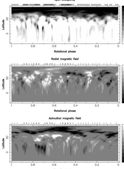
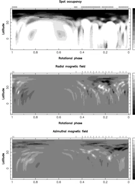
Figure 2. Maximum entropy brightness (upper row) and magnetic (lower rows) rectangular maps of AB Dor at epoch 1998.03. The reconstructed meridional field component is very small and is therefore not shown here. The vertical ticks above each graph depict the rotational phases of individual StokesIandV
observations. Positive field values correspond to magnetic vectors directed outward and eastward for radial and azimuthal field components, respectively (all labelled in G). Note that the rotational phase runs backwards (i.e. from right to left) on all maps.
Table 4. Radial velocities of AB Dor and LQ Hya (columns 2 and 3), sys-temic velocity of HR 1099 (column 4), and orbital phase of first conjunction of HR 1099 (column 5) in the ephemeris of Fekel (1983), for each of our ob-serving runs. The rms accuracy on radial velocities is of the order of 0.2 km s−1(the stellar lines being broad and time variable), while the error bar on
the phase of first conjunction is always smaller than 0.0001.
Epoch vrad φ0
(km s−1)
AB Dor LQ Hya HR 1099 HR 1099
1998.03 31.5 8.4 −14.5 −0.0458
1999.00 31.6 8.4 −14.6 −0.0529
1999.97 31.8 8.2 −14.7 −0.0616
2000.93 32.1 8.4 −14.8 −0.0701
2001.99 32.7 8.6 −14.5 −0.0784
error bar for us to claim that it is real. It very probably reflects the orbital motion of AB Dor recently demonstrated by Guirado et al. (1997), and continuous monitoring should help to determine what the orbital period actually is.
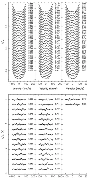
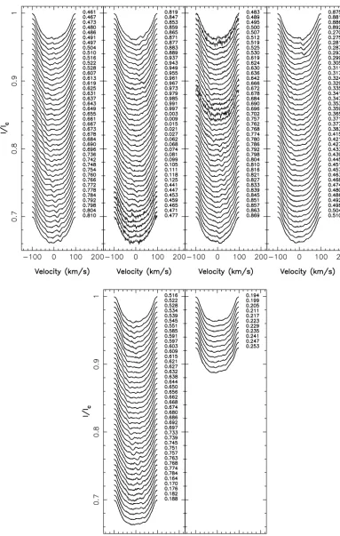
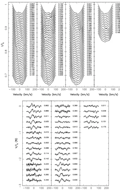
All data sets (phased according to Innis et al.’s 1988 ephemeris HJD=244 4296.575+0.514 79 E) provide very good to excellent sampling of the rotational cycle of AB Dor, except that collected at epoch 1999.97 for which bad weather (see Section 2.2) prevented us from covering more than approximately half the visible surface of AB Dor. The maximum entropy images we reconstruct from the var-ious data sets are shown in Figs 2, 4, 6, 8 and 10 for epochs 1998.03, 1999.00, 1999.97, 2000.93 and 2001.99, respectively, while the cor-responding fits are presented in Figs 3, 5, 7, 9 and 11. Unpolarized LSD profiles are fitted to an average accuracy level of approximately 0.07 per cent rms, while StokesVLSD profiles are adjusted at unit reducedχ2level.
Note that in some cases (e.g. between phase 0.4 and 0.7 at epoch 2001.99, see Fig. 11), we can clearly see in the observed StokesI LSD profiles a shallow, but significant, absorption feature travelling all the way throughout the line from the blue side to the red side of the profile, which is not reproduced in the synthetic profiles. We consider these spectral features as the first evidence for small regions brighter than the surrounding photosphere (i.e. faculae) located at the surface of AB Dor; indeed only bright surface features can pro-duce such absorption transients in the LSD line profiles, instead of the standard pseudo-emission bumps that cool star spots generate. Being designed for reconstructing only cool surface regions (to pre-vent bright artefacts from showing up in the image, see Cameron 1992), our code unsurprisingly fails at fitting these absorption trails in the dynamic spectra. Given that there are very few such regions on AB Dor at any given epoch, this is not a significant limitation for the present study, the aim of which is to delineate the structure of the magnetic field and its long-term evolution.
All brightness images are structurally very similar, with a main polar spot and a large number (more than 25 at epoch 2001.99) of small mid- to low-latitude appendages or separate spots, some of them reconstructed very close or even below the equator. They all yield very similar spot coverage, of the order of 8.5 per cent of the total stellar surface, with approximately one-third of the spots lo-cated at a latitude lower than 50◦. A closer analysis reveals that the relative fraction of the spot coverage associated with low-latitude features (i.e. lower than 50◦) with respect to that of circumpolar re-gions increased slightly but regularly over our observing time-span of 5 yr, from approximately 25 per cent at epoch 1998.03 up to 40 per cent at epoch 2001.99. Looking at the yearly transformation of curves such as that shown in the left-hand panel of Fig. 12 and
notic-ing, in particular, that the peak at high latitude in the distribution of the fractional spot coverage does not become progressively broader with time towards low latitudes, we can conclude that this evolution essentially reflects a global modification of the spot configuration occurring on a long-term basis, with a polar spot becoming pro-gressively weaker with time and more/bigger spots forming at low latitudes, rather than of some slow migration pattern of high-latitude features towards the equator.
The same global similarity with previously reconstructed maps is observed on the magnetic images as well.3These maps yield mean
quadratic magnetic fluxes (defined here as the local field modulus times the local relative surface area, regardless of the field orienta-tion) of the order of 125 G at most epochs, with a peak to 175 G at epoch 2001.99. Only at epoch 1999.97 is the mean field as low as 60 G, owing to the poor phase coverage that prevented us from re-constructing more than approximately half the visible surface of the star. Comparing with values obtained at epoch 1995.94 and 1996.99 (both equal to approximately 110 G, Donati et al. 1999), we can conclude that the field flux of AB Dor has regularly increased up to now. We also find that approximately 60–70 per cent of the quadratic magnetic flux is recovered at a latitude lower than 50◦. The clear difference with the brightness images (for which only one-third of the total spottedness is found at latitudes lower than 50◦) may be caused, at least partly, by the fact that some of the magnetic flux lo-cated close to the visible pole is obscured by the relative darkness of the huge polar spot. Indeed, almost no magnetic flux is recovered at latitudes higher than 80◦(see the left-hand panel of Fig. 12), where the local surface brightness never exceeds 20 per cent of that in the quiet photosphere.
The most striking similarity with previous maps is of course the ring of clockwise field surrounding the rotational pole of AB Dor, showing up very clearly in every single image. However, the lati-tudinal polarity pattern of the azimuthal field component at lower latitudes that we reported in the previous maps (counterclockwise field at intermediate latitudes and clockwise field close to the equa-tor) seems less obvious in this new sequence of maps. Although we still statistically tend to find regions with strongest positive az-imuthal field at intermediate latitudes, we also sometimes find a few of them close to the equator (e.g. at phase 0.58 on epoch 1998.03, or at phase 0.87 on epoch 2000.93), and several regions of intense clockwise azimuthal field at intermediate latitudes (e.g. at phase 0.24 on epoch 2001.99). If we average all maps together and inte-grate the algebraic azimuthal flux over longitudes (see the dash-dot curve in left-hand panel of Fig. 12), we confirm that there are in-deed, statistically at least, two dominant azimuthal field polarities throughout the upper hemisphere of AB Dor, a negative one at a latitude of approximately 70◦ (the circumpolar ring of clockwise field), and a second negative one at a latitude of approximately 15◦. A third one with opposite polarity shows up marginally between the two others, at a latitude of approximately 35◦.
This result therefore confirms the suspicion reported in our pre-vious studies, i.e. that the azimuthal field component essentially represents the mainly axisymmetric, dynamo generated, large-scale toroidal field structure, which, for some yet unknown reason, is not
3The impression that magnetic maps feature a finer spatial resolution than
brightness maps, for instance at epoch 2001.99 (see Fig. 10), is only a visual artefact of the displayed contours, autocorrelation maps of reconstructed images demonstrating clearly that the spatial resolution of magnetic maps is approximately 3 times lower than that of brightness maps, as expected from the much poorer phase sampling of the StokesVdata.
Dynamo processes and activity cycles
1155
Figure 3. Maximum entropy fit (thick line) to the observed (thin line) StokesI(top panel) andV(bottom panel) data sets. Observations are depicted from top to bottom and left to right by increasingUTdate (with successive profiles being shifted downwards for graphical purposes). The dotted lines in the bottom panel illustrate the zero circular polarization level of each profile. Rotational phases are indicated to the right of each profile.
Figure 4. Same as in Fig. 2 for epoch 1999.00. confined at the base of the convective zone as in the Sun, but
read-ily detectable at photospheric level and thus probably distributed throughout the whole convective zone. We stress, however, that, at each epoch, a significant fraction of the azimuthal field we recon-struct at low to intermediate latitudes does not contribute to this
axisymmetric structure, but rather to a more complex, higher-order, component of the large-scale toroidal dynamo field. No temporal evolution of the latitudinal position of these polarities is readily visi-ble from the images; splitting all epochs into two consecutive subsets and comparing the resulting latitudinal magnetic flux distributions
Dynamo processes and activity cycles
1157
Figure 5. Same as in Fig. 3 for epoch 1999.00. of the azimuthal field yields no evidence for the potential migration
of these rings over the full time-span of our observations. The radial field maps are also structurally similar to their 1995 and 1996 equivalents, showing no apparent latitudinal polarity
pat-tern. However, if we proceed as we did for the azimuthal field image, i.e. by integrating the radial field images over longitudes to retain only the axisymmetric latitudinal pattern (presumably linked to the poloidal component of the large-scale dynamo field), we observe
Figure 5–continued
that the polarity at low latitudes remained essentially positive at all epochs, while that at high latitudes switched sign (from neg-ative to positive) sometimes around epoch 1999.5. Note that this sign switch at high latitudes is readily visible in the Doppler images themselves; the prominent spot of negative radial field reconstructed at epoch 1998.03 (at phase 0.55 and latitude 70◦) is replaced approx-imately 3 yr later by a region of positive radial field with similar size (located at phase 0.90 and latitude 65◦), while all other maps essentially feature mixed polarity (and usually much smaller sized) radial field regions at such a high latitude. This temporal change of the latitudinal polarity structure of the radial field looks promising for investigations of the long-term, possibly cyclic, evolution of the large-scale dynamo field and is discussed further in Section 6.
Another quantity worth computing is the fraction of the total mag-netic energy stored in the various field components. We find that on average, the radial field component contains approximately 40 per cent of the reconstructed magnetic energy, varying from approxi-mately 35 to 45 per cent depending on the epoch. As our imaging technique is not very sensitive to meridional fields for stars with high inclination angles (Donati & Brown 1997), we find, unsurpris-ingly, that the azimuthal field component contains approximately 60 per cent of the total magnetic energy. At two different epochs since the beginning of our observations, however, (in 1995.94 and 1999.97), the radial field component is found to dominate the mag-netic energy budget, including as much as 55 per cent of the total magnetic energy. The first question that arises is of course to know whether the quantities we estimated, and in particular their temporal fluctuations, are indeed representative of some real process going on at the surface of the star, or only reflect the intrinsic limitations of the imaging code (recalled in Section 2.3). One could for instance argue that a lot of the magnetic field present at the surface of the star (possibly even the major fraction of it) is concentrated in cool
regions or in small-scale bipolar features that are not reconstructed (or at least strongly dimmed) in our images. Although this is indeed possible, it does not necessarily imply that the relative amounts we derive for the magnetic energies stored in each field component and their fluctuations with time are meaningless; one could fairly rea-sonably imagine that both small- and large-scale magnetic features follow the same variational laws (as for instance on the Sun where the Hale polarity law applies for large active regions and for small ephemeral features), with their respective weights being dictated by some constraint of physical origin (e.g. that the distribution of the spatial scales of magnetic features is a fractal of fixed dimension). Another concern deals with the possible impact of phase coverage on the derived ratio of reconstructed radial and azimuthal magnetic field energies; simulations indicate that only very weak dependence should be observed, validating our result that the large-scale mag-netic structures are probably indeed truly variable along the lines described above, even in the case of epoch 1999.97 at which the data set is sparser than usual. Although we keep further discussion on this subject for Section 6, we already stress the fact that this tem-poral fluctuation between the azimuthal and the radial components of the medium- to large-scale magnetic field that our data suggest represents an interesting discovery and a potentially fruitful source of information for our understanding of how dynamos operate in cool stars other than the Sun.
If we now look at how the brightness and quadratic magnetic flux distributions depend on longitude once integrated over latitudes 0◦– 50◦(i.e. keeping the polar regions out to concentrate on low-latitude features and avoid contamination from the tilted polar spot, see be-low), we find that both curves usually show one main peak roughly centred on the same longitude (see, for instance, the right-hand panel of Fig. 12 in the particular case of epoch 2001.99). At some particu-lar epochs (e.g. 1998.03), one of these distributions may even feature
Dynamo processes and activity cycles
1159
Figure 6. Same as in Fig. 2 for epoch 1999.97. a second, usually weaker, peak. Concentrating on the longitudinal
pattern of the magnetic flux, we find that the main peak, whenever clearly visible (i.e. at epochs 1995.94, 1996.99, 1998.03, 2000.93 and 2001.99), is located at phase 0.81, 0.69, 0.70, 0.97 and 0.37, respectively. We interpret these coincident peaks in both brightness
and magnetic flux distributions with longitudes as evidence for ‘ac-tive longitudes’ at the surface of AB Dor, presumably linked to an angular tilt in the dipolar component of the large-scale dynamo field. Note that such active longitudes are not necessarily equivalent to (and in particular are not defined in the same way as) those invoked
Figure 7. Same as in Fig. 3 for epoch 1999.97. by other authors (e.g. Jetsu, Pelt & Tuominen 1993; Berdyugina,
Pelt & Tumoninen 2002), for whom they represent longitudes at which cool spots tend to form more often. We speculate that these phases of enhanced activity probably relate to the open field regions of the global magnetic topology of AB Dor that Jardine, Cameron & Donati (2002) recently demonstrated. The long-term evolution of this active longitude does not, however, seem to follow any obvious trend up to now. A more detailed analysis, involving in particular spherical harmonics reconstruction of the magnetic field map (e.g. Donati 2001) and field extrapolation (e.g. Jardine et al. 2002), is probably required to investigate this issue properly.
In addition to this, at most epochs we observe a clear angular off-centring of the azimuthal field ring encircling the rotational pole of AB Dor, and a tilt of the cool polar spot, by approximately 10◦. One can reasonably wonder whether these tilts of both the brightness and magnetic distributions are somehow related to the active longitude mentioned above. However, we observe that, for most epochs, the phases towards which the azimuthal field ring and the polar spot are tilted are mutually incompatible (being, respectively, equal to 0.45 and 0.88 at epoch 1996.99 for instance, Donati et al. 1999); more-over, both often also disagree with the phase of enhanced activity that we determined previously (equal to 0.69 at epoch 1996.99). The reason for this apparent contradiction, suggesting in particular, that the large-scale brightness and magnetic field distributions may be misaligned, is not yet clear.
4 T H E Y O U N G K 0 DWA R F L Q H Y D R A E
For all reconstructions presented herein, we assumed for LQ Hya the same inclination angle as that used in Donati (1999), equal to 60◦. As for AB Dor, the line-of-sight projected rotational velocity we used in this study (26 km s−1) is slightly smaller than what we
used in our previous investigation (Donati 1999, wherevsiniwas
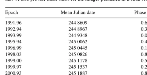
Table 5. Approximate phase shifts to be subtracted to our sets of phases to convert them into those produced by Jetsu et al.’s ephemeris (1993). Note that we also provide these shifts for the images published in Donati (1999).
Epoch Mean Julian date Phase shift
1991.96 244 8609 0.68
1992.94 244 8967 0.35
1993.99 244 9348 0.07
1995.94 245 0062 0.42
1996.99 245 0445 0.15
1998.03 245 0826 0.87
1999.00 245 1178 0.53
1999.97 245 1537 0.21
2000.93 245 1887 0.88
2001.99 245 2271 0.60
set to 26.5 km s−1); we find, in particular, that this value enables us
to obtain a better fit to the data and to minimize systematic residuals, at the cost of producing brightness images with slightly larger spot coverage. The radial velocity we derive for LQ Hya is remarkably constant. If we incorporate the values derived by reprocessing with the same software the data secured during the 1995 December and 1996 December runs (both equal to 8.5±0.2 km s−1), we find that
LQ Hya drifts away from the Sun at a velocity of 8.4±0.2 km s−1. In
particular, it implies that LQ Hya is very likely not a binary star. All data were phased according to the ephemeris of Strassmeier et al. (1993) (HJD=244 8270.0+1.606 E) in order to remain consistent with the previous studies of the same kind (Donati 1999). To make our results more easily comparable with those of other studies (e.g. Berdyugina et al. 2002) using a different ephemeris (that of Jetsu et al. 1993), we provide a list of all phase shifts (see Table 5) to allow any potential reader to compare the results of both studies more easily.
[image:16.612.308.547.420.542.2]Dynamo processes and activity cycles
1161
Figure 8. Same as in Fig. 2 for epoch 2000.93.
We also made the assumption that no surface differential rotation is present on LQ Hya; although this is most likely wrong (given, in particular, the increasing body of evidence that cool stars do in-deed possess solar-like differential rotation; e.g. Donati & Cameron
1997; Donati et al. 2000), this is nevertheless not a major problem for us given the small time-span of our observations. The effect of assuming, in the reconstruction process, that the star rotates as a solid body (with a rate of 3.912 rad d−1, i.e. close to that estimated
Figure 9. Same as in Fig. 3 for epoch 2000.93. for the main non-axisymmetric spot groups, centred at a latitude of
approximately 35◦, see Donati et al. 2003) is indeed that the fea-tures we recover are slightly blurred, by an amount that depends on the latitudinal distance from 35◦. For an average differential
rotation rate between the equator and pole of approximately 0.1 rad d−1(Donati et al. 2003) and a maximum time-span of 13 d,
we find that spots located at latitudes of either 20◦ or 70◦are az-imuthally blurred by no more than a few per cent of the rotation
Dynamo processes and activity cycles
1163
Figure 10. Same as in Fig. 2 for epoch 2001.99. cycle towards both sides of the position at which they are
im-aged. This is not a very limiting factor in the particular case of LQ Hya; the lowvsini of this star and the spectral resolution of our observations indeed constrains the size of any spatially resolved structure reconstructed at its surface to be larger than 3 and 9 per
cent in rotational phase, for latitudes of 20◦and 70◦, respectively. Moreover, this problem does not prevent us from examining the global structure of the magnetic field and its axisymmetric com-ponents, and from looking for the potential long-term evolution of the field. A careful investigation of these data to estimate the
Figure 11. Same as in Fig. 3 for epoch 2001.99. surface differential rotation of LQ Hya is presented in Donati
et al. (2003).
The phase coverage that we achieved at each epoch essentially reflects the amount of clear time in each observing session (see
Section 2.2), i.e. reasonable to excellent on 1999.00, 2000.93 and 1999.97, moderate on 1998.03 but very poor on 1999.97. The maximum entropy images we obtain from the different data sets are shown in Figs 13–17 for epochs 1998.03, 1999.00, 1999.97,
Dynamo processes and activity cycles
1165
Figure 11–continued
2000.93 and 2001.99, respectively, along with the corresponding fits to the observed LSD profiles. Unpolarized LSD profiles are fitted to an average accuracy level of approximately 0.1 per cent rms, while StokesV LSD profiles are adjusted at unit reducedχ2
level.
Figure 12. Fractional spot coverage (full line) and quadratic magnetic flux in kG (dashed line) per latitude bin (after integrating over longitudes, left-hand panel) or per rotational phase bin (after integrating over latitudes 0◦–50◦, right-hand panel). Note that the quadratic magnetic flux is defined here as the local field modulus times the local relative surface area, regardless of the field orientation. In the left-hand panel, the dash-dot line depicts the azimuthal field flux per latitude bin in kG, once integrated over longitudes (we do not show the average radial field flux with latitude, since this quantity is observed to vary significantly with time at high latitudes, see the text). The right-hand curves correspond to epoch 2001.99, while the left-hand ones represent an average over all observing epochs (including 1995 December and 1996 December). Note that the sharp decline of all curves towards the pole reflects no more than decreasing the relative surface of constant latitude belts with increasing latitude.
Again, the brightness images we reconstruct are structurally very similar to those presented in Donati (1999), featuring one main polar spot with a small number of (usually approximately five) low-latitude spots, either fully detached from, or appearing as extensions of, the cool polar cap. We also note that these images share some
[image:21.612.46.551.473.661.2]Figure 13. Top panel, maximum entropy brightness (upper left) and magnetic field images of the young K0 dwarf LQ Hya at epoch 1998.03. These images are flattened polar projections extending down to a latitude of−30◦(the bold and thin circles depicting the equator and the 30◦and 60◦ latitude parallels, respectively). The radial ticks around (and outside) each plot illustrate the phases at which the star was observed. Positive field values correspond to magnetic vectors directed outward, anticlockwise and poleward for radial, azimuthal and meridional field components, respectively (all labelled in G). Bottom panel: maximum entropy fit (thick line) to the observed (thin line) StokesI(left) andV(right) data sets.
Dynamo processes and activity cycles
1167
Figure 14. Same as in Fig. 13 for epoch 1999.00. similarity with those derived for AB Dor, if we take into account
the fact that the latter are much better spatially resolved, by a factor of at least 3.5 (assuming dense phase coverage) and often signifi-cantly more (within phase gaps of the data set). Another probable consequence of this different spatial resolution is that the amount
of spot we recover is significantly smaller for LQ Hya than for AB Dor; while the first three epochs suggest a spot coverage of only approximately 3.2 per cent of the total stellar surface, the last two indicate a slightly higher value of approximately 4.4 per cent, proba-bly reflecting the much better coverage obtained during these recent
Figure 15. Same as in Fig. 13 for epoch 1999.97.
campaigns. Although this variation looks consistent with the global dimming of the integrated flux from LQ Hya between epoch 1995 and 2000 (Berdyugina et al. 2002), the actual decrease in bright-ness revealed by photometry (0.1 mag) is much larger that the 1 per
cent increase in spot coverage that we derive here, strengthening the conclusion that Doppler images reconstructed without photometric information cannot be trusted for predicting long-term stellar irra-diance variations.
Dynamo processes and activity cycles
1169
Figure 16. Same as in Fig. 13 for epoch 2000.93.
In the same spirit, comparing the images derived by Berdyugina et al. (2002) from photometric data only with ours (at least those obtained with very good phase coverage, i.e. at epoch 1999.00, 2000.93 and 2001.99) is very instructive as well. The light curve
of LQ Hya around epoch 1999.00 is basically flat (slightly deeper in the first half rotation cycle in Jetsu et al.’s ephemeris, i.e. from phase 0.53 to 1.03 in the ephemeris we used), arguing in favour of a roughly axisymmetric distribution of low-latitude features at
Figure 16–continued
the surface of the star (with slightly more features in the second half rotation cycle in the ephemeris we used). This is indeed grossly what we obtain from our own image (see Fig. 14). At epoch 2000.93 and 2001.99, however, the situation is very different; while the light curves of Berdyugina et al. (2002) indicate that LQ Hya reaches maximum brightness (and thus presumably minimum low-latitude spottedness) around phases 0.70 and 0.55 at epochs 2000.93 and 2001.99, respectively (in Jetsu et al.’s ephemeris, corresponding to a phase of 0.58 and 0.15, respectively, in the ephemeris we used), our images demonstrate that, in both cases, this phase almost coin-cides with that of one of the main groups of low-latitude features reconstructed at the surface of the star (those at phase 0.55 and 0.20 at epoch 2000.93 and 2001.99, respectively, see Figs 16 and 17). Similarly, phases of minimum brightness (and thus presum-ably maximum low-latitude spottedness) at epoch 2001.99 (roughly equal to 0.25 and 0.75 in Jetsu et al.’s ephemeris, and to 0.85 and 0.35 in our ephemeris) appear to correspond with regions that are basically free of low-latitude spots in our reconstructed image (see Fig. 17). Note that our intention is certainly not to question the ac-curacy of Berdyugina et al.’s (2002) photometric data; our images demonstrate, however, that their implicit assumption that phases of maximum and minimum photometric brightness, respectively, correspond to regions with the highest and lowest density of low-latitude cool spots at the surface of the star is simply invalid. Our images point out that the shape of the resulting light curve results from many different factors, with high-latitude features (e.g. the off-centring of the polar spot) playing as important a role as that of low-latitude ones. A similar conclusion was reached in Vogt et al. (1999) from comparing light curves with Doppler images derived from spectroscopy.
The average latitudinal pattern of all spot distributions since 1995 December, shown on the left-hand panel of Fig. 18, is found to be rather similar to that of AB Dor, but with slightly more spots (ap-proximately half of them) appearing at a latitude lower than 50◦, the other half forming the polar cap. In particular, it is worth not-ing the fact that low-latitude spots seem to appear preferentially around latitude 25◦. A closer look at these images, and those from
epoch 1995.94 and 1996.99, reveals that the fractional spottedness associated with the polar cap actually varies slightly with time; after decreasing regularly down to a minimum (of approximately 40 per cent) reached at epoch 1998.03, it increased again back up to its apparently nominal value (of approximately 55 per cent) where it stayed for the last 3 yr. As for AB Dor, this long-term varia-tion of the latitudinal spot repartivaria-tion at the surface of LQ Hya does not seem to be caused by a progressive migration of high-latitude features towards the equator, but rather by a slow, possibly periodic, phenomenon of yet unknown origin that changes the re-spective average sizes of newly emerging low- and high-latitude features.
The magnetic images we reconstruct for LQ Hya are