Potential impacts of precipitation change on large-scale patterns of tree diversity

This is a repository copy of

Potential impacts of precipitation change on large-scale

patterns of tree diversity

.

White Rose Research Online URL for this paper:

http://eprints.whiterose.ac.uk/78944/

Article:

Konar, M, Muneepeerakul, R, Azaele, S et al. (3 more authors) (2010) Potential impacts of

precipitation change on large-scale patterns of tree diversity. Water Resources Research,

46 (11). W11515. ISSN 0043-1397

https://doi.org/10.1029/2010WR009384

eprints@whiterose.ac.uk https://eprints.whiterose.ac.uk/ Reuse

Unless indicated otherwise, fulltext items are protected by copyright with all rights reserved. The copyright exception in section 29 of the Copyright, Designs and Patents Act 1988 allows the making of a single copy solely for the purpose of non-commercial research or private study within the limits of fair dealing. The publisher or other rights-holder may allow further reproduction and re-use of this version - refer to the White Rose Research Online record for this item. Where records identify the publisher as the copyright holder, users can verify any specific terms of use on the publisher’s website.

Takedown

If you consider content in White Rose Research Online to be in breach of UK law, please notify us by

Potential impacts of precipitation change on large

‐

scale

patterns of tree diversity

M. Konar,

_{R. Muneepeerakul,}

_{S. Azaele,}

_{E. Bertuzzo,}

_{A. Rinaldo,}

and I. Rodriguez

‐

Iturbe

Received 2 April 2010; revised 5 July 2010; accepted 20 July 2010; published 9 November 2010.

[1]

Forests are globally important ecosystems host to outstanding biological diversity.

Widespread efforts have addressed the impacts of climate change on biodiversity in these

ecosystems. We show that a metacommunity model founded on basic ecological processes

offers direct linkage from large

‐

scale forcing, such as precipitation, to tree diversity patterns

of the Mississippi

‐

Missouri River System and its subregions. We quantify changes in tree

diversity patterns under various projected precipitation patterns, resulting in a range of

responses. Uncertainties accompanying global climate models necessitate the use of

scenarios of biodiversity. Here we present results from scenarios with the largest losses

and gains in tree diversity. Our results suggest that species losses under scenarios with the

most dramatic contractions tend to be greater in magnitude, spatial extent, and statistical

significance than gains under alternative scenarios. These findings are expected to have

important implications for conservation policy and resource management.

Citation: Konar, M., R. Muneepeerakul, S. Azaele, E. Bertuzzo, A. Rinaldo, and I. Rodriguez‐Iturbe (2010), Potential impacts of precipitation change on large‐scale patterns of tree diversity,Water Resour. Res.,46, W11515, doi:10.1029/2010WR009384.

1.

Introduction

[2] Climate change is recognized as a major threat to bio-diversity [Walther et al., 2002;Rockström et al., 2009] and is likely to be the most significant factor following land‐use

changes [Sala et al., 2000]. Quantification of the potential impacts of climate change on biodiversity is urgently needed [Millenium Ecosystem Assessment, 2005;Sala et al., 2000; Clark et al., 2001;Botkin et al., 2007]. However, climate change encompasses many factors (e.g., temperature, pre-cipitation patterns, CO2concentration) that are anticipated to affect different species in different manners, owing to the fact that species react in unique and oftentimes unpredictable ways to changes in their environment, making it particularly challenging to model.

[3] Spatial scale is an important consideration when studying the impact of climate change on biodiversity, since climate change projections are provided at large spatial scales [Intergovernmental Panel on Climate Change, 2007] (see also Coupled Model Intercomparison Project 3, Statistically downscaled WCRP CMIP3 climate projections, 2009, http:// gdo‐dcp.ucllnl.org/downscaled_cmip3_projections), while

diversity models are scale‐dependent. One of the oldest and

best‐documented patterns in community ecology is the

species‐area curve, which describes the observed increase in

species richness as area increases [Rosenzweig, 1995]. While

the general pattern of increased diversity with area is widely accepted, the mechanisms driving this relationship are still debated. This relationship has long fascinated ecologists, and there is an extensive literature devoted to exploring the scale dependence of diversity patterns [Currie, 1991;Crawley and Harral, 2001;Hui, 2009]. Accordingly, when coupling bio-diversity models with climate change research, the spatial scale of the biodiversity model must be appropriate for use with the climate models.

[4] For the past decade, species distribution models have been widely used to study the impact of climate change on biodiversity [Guisan and Thuiller, 2005;Morin and Thuiller, 2009]. Many of these models simply rely on correlations between environmental variables (especially climatic variables, i.e., bioclimate envelope models) and species distribution. These correlations are then used to predict potential distribu-tion of species under future climates. Many widely acknowl-edged uncertainties accompany these forecasts [Pearson and Dawson, 2003; Thuiller et al., 2008; Fitzpatrick and Hargrove, 2009], such as applying correlations derived from present conditions to novel climates [Ibanez et al., 2006].

[5] An approach based upon ecological processes would complement species distribution models in predicting the impact of climate change on biodiversity [Jeltsch et al., 2008; Algar et al., 2009], particularly one founded on key demo-graphic rates (e.g., birth, death, dispersal, and immigration), such as the neutral theory of biodiversity [Hubbell, 2001]. Neutral models are based on stochastic demographic pro-cesses and treat individuals as equivalent in their per capita rates of birth, death, and speciation. As such, neutral models do not incorporate unique ecological characteristics of spe-cies; nonetheless, they have produced excellent fits to data and are particularly well suited to modeling large‐scale spatial

biodiversity patterns [Muneepeerakul et al., 2008;Bertuzzo et al., 2009].

1_{Department of Civil and Environmental Engineering,Princeton} University, Princeton, New Jersey, USA.

2_{Laboratorie of E´cohydrology,Ecole Polytechnique Fédérale, Lausanne,} Switzerland.

3

Department IMAGE and International Centre for Hydrology “Dino Tonini,”Università di Padova, Padua, Italy.

[6] The Mississippi‐Missouri River System (MMRS) is the

largest watershed in North America and among the largest in the world, covering 2,980,000 km2, approximately 40% of the continental United States (Figure 1). This watershed encompasses a diverse suite of environmental gradients, forest ecosystems, establishment history, and anthropogenic disturbances, thereby complicating ecological forecasts. Yet, projecting biodiversity patterns in the MMRS is crucial as part of a comprehensive evaluation of the impact of climate change over the United States.

[7] In this study, we first implement a neutral metacom-munity model of tree diversity in the MMRS and five sub-regions to investigate its ability to capture the large‐scale

biodiversity patterns of these systems. The appealing feature of this modeling approach is its potential to provide a single, coherent framework within which we can study multiple diversity patterns simultaneously [Muneepeerakul et al., 2008;Bertuzzo et al., 2009]. Once the ability of the neutral model to capture the empirical patterns has been validated, we proceed to quantify changes in biodiversity patterns by forcing the model with precipitation patterns given by global climate models. Here we use precipitation, among other possible controlling variables, as the key variable to capture the main dynamics of climate change responsible for tree diversity patterns at large spatial scales. Note that in this paper, we only model and consider the impact of climate change on tree species diversity, and not on other plant functional types or on ecosystem diversity more generally.

2.

Data and Methods

2.1. Analysis of Empirical Tree Data

[8] In the following analysis, the 824 direct tributary areas (DTAs) comprising the MMRS are populated with occur-rence data of 231 tree species from the U.S. Forest Service Forest Inventory and Analysis Database [U.S. Forest Service, 2008]. Each DTA is a subbasin of the MMRS as defined by the U.S. National Hydrography Database at the HUC‐8 scale

[National Hydrography Dataset, 2008].

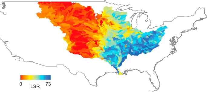
[9] The data were combined and analyzed for two key biodiversity signatures. First, we consider the distribution of local species richness (LSR). LSR is simply the number of species found in a DTA. The spatial distribution of LSR in the MMRS is shown in Figure 1, and its corresponding histogram

is shown in Figure 4. The frequency distribution of LSR is bimodal due to environmental heterogeneity, such that the species‐rich DTAs contributing to the peak around 40–

50 species are those east of the 100°W meridian, a location known for sharp changes in annual precipitation [e.g., Dingman, 2002], while those in the West make up the spe-cies‐poor peak in the histogram. Second, we consider the

species rank occupancy, the number of DTAs in which a particular species is found as a function of its rank.

2.2. Neutral Metacommunity Model

[10] We implemented a spatially explicit neutral meta-community model in the MMRS. According to ecological neutral dynamics [Hubbell, 2001], all basic ecological pro-cesses implemented in the model (i.e., birth, death, immi-gration, dispersal, and colonization) are equivalent at a per capita level for all species. This modeling approach is attractive for its simplicity, parameter parsimony, and its ability to simultaneously produce several diversity patterns, which allows us to investigate the connection between these patterns.

[11] At every time step, a tree unit randomly selected from all tree units in the system dies, and the resources are freed up and available for colonization by another tree unit. With probabilityn (the diversification rate), the empty site is col-onized by a new species not already present in the system, while with the remaining probability, 1‐n, the empty site is colonized by a species already existing in the system. The colonization process is modeled through the dispersal of propagules produced by the tree units. The neutral theory assumes no species‐specific competitive advantages, and

therefore the probability that an empty site is colonized by a certain species depends only on the relative abundance of propagules of that species that have arrived, following the dispersal process, at the empty site. This modeling framework closely follows that of Muneepeerakul et al. [2008], with major differences to account for those between fish and tree systems.

[12] In our metacommunity model, the DTAs define the local communities of the system. Each DTA was assigned a tree habitat capacity, H. Habitat capacity is defined as the number of tree units able to exist in a local community, which is best approximated by the forest cover of a given DTA. For Figure 1. Map of local species richness (LSR) of trees in each direct tributary area (DTA) (i.e., at the

USGS HUC‐8 scale; refer to text) of the MMRS.

KONAR ET AL.: CLIMATE CHANGE IMPACTS ON TREE DIVERSITY W11515 W11515

this reason, habitat capacity is assumed to be proportional to forest area and is calculated asHi=CH(FA)i, rounded to the

nearest integer, whereCHis a constant of proportionality and

FAiis the forest area of DTAi. Every DTA is assumed to be

always saturated at its habitat capacity. Note that a larger habitat capacity, i.e., more tree units in a local community, generally corresponds with a higher LSR, though, as quan-titatively shown below, LSR also depends on several other important factors.

[13] Following the approach used inSankaran et al. [2005], we established a functional relationship for forest cover. To determine the variable that best determines habitat capacity at large spatial scales, we regressed forest cover with mean annual temperature, evapotranspiration, and precipita-tion for all DTAs in the MMRS. As shown in Figure 2, both evapotranspiration and precipitation provide acceptable options for the construction of a habitat capacity functional relationship. However, the functional relationship between forest cover and precipitation (Figure 2c) appears to exhibit a better‐defined upper bound. Thus, we decided to use mean

annual precipitation (MAP) as the indicator of habitat capacity at large spatial scales throughout the MMRS.

[14] The functional relationship between forest cover and mean annual precipitation was constructed using data from the U.S. Forest Service (Forest cover types, http://www. nationalatlas.gov/mld/foresti.html) and the Natural Resources Conservation Service (United States average annual pre-cipitation, 1961–1990, http://rnp782.er.usgs.gov/atlas2/mld/

prism0p.html) for all 824 DTAs. In the MMRS, potential forest cover (i.e., the solid curve shown in Figure 2c) grad-ually increases with MAP until reaching a plateau of 100% coverage around 900 mm. Here sites that fall below the upper bound are considered to do so as a result of anthropogenic (e.g., land‐use change) or environmental factors that prevent

the forest cover from reaching its potential value. Each of these sites is assigned a forest cover index,Ii, defined as the

ratio between actual and potential forest cover. Note thatIiis

not correlated with MAP.

[15] Dispersal kernels are used to determine how propa-gules move. In this model, the dispersal kernel (K) is assumed to take an exponential form and use Euclidean distances:Kij=

CCexp(−Dij/aC), whereKijis the fraction of propagules of

trees produced at DTAjarriving at DTAiafter dispersal,CC

normalization constant (∑i Kij = 1), Dij the between‐DTA

distance, anda_Cthe characteristic dispersal length.

[16] To allow tree propagules to move across the system boundaries as they do in real life, we have made the system boundaries permeable. In particular, in the model, such immigration across the boundary is included by makingn_i, the immigration rate at DTAi, a function of distance to the boundary and the habitat capacity of the associated boundary DTA: n_i = C_IH_b

i exp(−Dbi/aI), where Hbi and Dbi are the

habitat capacity of the boundary DTA closest to DTAiand the distance between them, respectively,CIthe normalization

constant (∑i n_i = ), the average number of immigrant species in one generation (defined as a period over which each tree unit dies once on average), and a_I the characteristic distance of immigration. The implicit assumption here is that diversification is dominated by immigration, and speciation is assumed negligible. Immigrating propagules move with their own exponential dispersal kernel, which is assumed to account for the aggregate movement of all individuals from outside the system. Hence, two exponential dispersal kernels are used in the model: one to represent movement within the system, with a characteristic length ofa_C, and another for immigration across the system boundary, with a characteristic length ofa_I.

[17] To determine the best‐fit parameter values, the model

is run for the entire MMRS, while the parameter values are tuned to fit the empirical patterns for each system of interest. The model as described above requires only four parameters for each system, namely,CH, a_C,a_I, and . The model is run until reaching a statistically steady state, after which the resulting patterns are averaged over 100 snapshots and then compared to the empirical ones.

2.3. Climate Change Impacts

[18] Of particular importance, our modeling framework permits direct linkage from various environmental changes to large‐scale biodiversity signatures. A common point of

con-fusion regarding the use of neutral models is that they ignore environmental variation. We would like to clarify this key point, since the ability to quantify the impacts of climate change on tree diversity is one of our main motivations in using a neutral model. Even though our model is neutral, it is still able to capture the impact of changing environmental drivers on tree diversity. Individuals in our neutral model do respond to environmental cues, they just do so in an equiva-lent manner.

[19] Here, to quantify the impact of climate change on large‐scale tree diversity characteristics, we map projected

precipitation patterns as given by the Coupled Model Inter-comparison Project 3 (CMIP3) climate models to new values of habitat capacity. The projected mean annual precipitation from 2049–2099 was used to obtain new values of habitat

capacity under climate change for the 824 DTAs in the MMRS (see http://gdo_‐dcp.ucllnl.org/downscaled_cmip3_ projections). We selected 15 statistically downscaled climate projections from the emissions path A2, the most extreme emissions pathway [Intergovernmental Panel on Climate Change, 2007]. Note that recent carbon dioxide emissions are actually above the A2 scenario, indicating that it may, in fact, be more conservative than initially thought, though future emissions remain uncertain [Karl et al., 2009]. The average MAP for each system considered in the study (MMRS, North, East, South, Southwest, and Northwest) under each CMIP3 climate model is summarized in Table 1.

[20] For each of the 15 climate change scenarios, the pro-jected MAP for DTAiwas used in Figure 2c to obtain a new potential forest cover for DTAi(see the next paragraph). The new potential forest cover was used in the equation Hi =

CHPiIito calculate the habitat capacity of DTAi,Hi, under

climate change, wherePidenotes potential forest area andIi

the forest cover index of DTAi, assumed to remain the same under climate change.CHis kept constant between the current

climate and climate change scenarios in the calculation ofH. This ensures that any differences between model realizations are due to climate change. With these resulting new habitat capacities, we are able to quantify how various climate change scenarios will affect large‐scale signatures of

biodi-versity under the neutral assumption. Note that no predictions are made with regard to specific species, since we are using a neutral model.

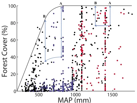
[21] Figure 3 is a schematic of how Piwas obtained. Pi

under the current climate scenario is depicted by points“A”.

These points correspond to the upper bound of the function for the MAP under the current climate scenario. To obtain the Pivalue for the climate change scenario, the projected MAP

for DTAiis located on the graph and the new corresponding potential forest cover is noted. New values of Pi are

represented in Figure 3 by points “B.” These procedures

were performed for the 824 DTAs across all 15 climate change scenarios.

3.

Results and Discussion

[22] Here we first demonstrate that our neutral meta-community model can reproduce key biodiversity patterns of

Table 1. Mean Annual Precipitation (MAP) of the Systems Considered in This Study for the Current Climate Scenario and Fifteen Climate Change Scenariosa

Scenario MMRS North Southwest East South Northwest

Current 790.08 831.62 571.38 1177.27 1237.87 432.70 BCCR‐BCM2.0 840.73 898.64 515.04 1360.49 1301.49 460.07 CGCM3.1 (T47) 901.58 963.37 584.28 1356.10 1370.95 527.48 CNRM‐CM3 778.80 882.67 436.89 1295.90 1176.41 440.99 CSIRO‐Mk3.0 853.54 918.88 581.37 1292.85 1279.78 489.99 GFDL‐CM2.0 711.61 784.22 382.52 1203.40 1062.83 411.35 GISS‐ER 899.59 1032.24 508.99 1479.87 1418.20 451.23 INM‐CM3.0 709.41 777.85 467.90 1069.25 1058.09 412.90 IPSL‐CM4 715.84 784.20 477.33 1089.84 1001.62 428.19 MIROC3.2 654.41 684.62 412.58 1040.21 994.41 355.29

ECHO‐G 868.32 918.59 646.06 1283.78 1337.44 485.51 ECHAM5/MPI‐OM 850.37 911.29 554.26 1339.91 1303.14 463.10 MRI‐CGCM2.3.2 868.41 965.67 571.59 1316.05 1350.87 480.27

CCSM3 890.18 930.47 614.50 1396.40 1358.08 496.96

PCM 887.12 898.73 644.60 1335.32 1321.70 526.24

UKMO‐HadCM3 795.37 824.48 488.05 1297.19 1231.82 437.27

a_{All values are in mm. Nomenclature of the climate change scenarios follows that of CMIP3. Bold numbers indicate the species} ‐ poor climate change scenario for a given system (red in Figures 5 and 6), and italic numbers indicate the species‐rich climate change scenario (blue in Figures 5 and 6).

Figure 3. Schematic of how habitat capacity was calculated under climate change. The mean annual precipitation (MAP) for each DTA under every scenario was located on the graph; only data points from the current climate scenario are shown here. The corresponding potential forest cover (Pi) was

deter-mined as the upper bound of the function. As an example, points A in the figure indicate the potential forest cover under the current climate scenario, while points B indicate the new potential forest cover under climate change. This new poten-tial forest cover was then multiplied by the forest cover index (Ii) to calculate the habitat capacity under each climate change

scenario. This was done for all 824 DTA data points in all 15 climate change scenarios. Blue points indicate DTAs in the North regions, red points the South region, and black points the rest.

KONAR ET AL.: CLIMATE CHANGE IMPACTS ON TREE DIVERSITY W11515 W11515

trees in the entire MMRS as well as its five different sub-regions. Indeed, this is a necessary condition to use this model to investigate the impact of climate change scenarios on macrobiodiversity characteristics. We then provide cli-mate change results for each system (i.e., the MMRS and its subregions).

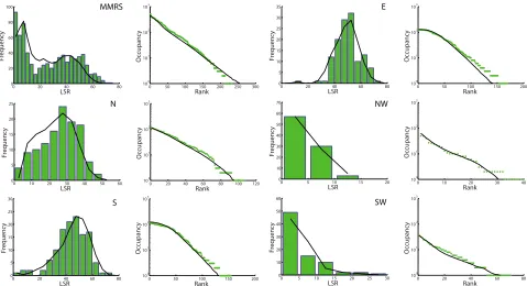
[23] As illustrated in Figure 4, the model provides an excellent fit to the LSR frequency distribution and rank‐

occupancy curve of the MMRS. When the parameters are recalibrated, i.e., tuned independently for each system, the model also captures the biodiversity patterns in the sub-regions quite well. The simultaneous good fits of patterns shown here indicate that mean annual precipitation provides a simple and effective characterization of habitat capacity. It is noteworthy that mean annual precipitation alone accurately characterizes habitat capacity in our model, rather than a more complex combination of environmental variables. This is desirable, since using a single variable to characterize habitat capacity maintains the model’s simplicity and parameter

parsimony and allows for a clear interpretation of the results. [24] We have shown that a simple neutral metacommunity model, coupled with an appropriate habitat capacity distri-bution and dispersal kernel, is able to reproduce major empirical tree diversity patterns in the MMRS. Since the model is able to reproduce several characteristic patterns simultaneously, it is likely capturing some of the underlying processes. When an agent‐based model, such as this neutral

metacommunity model, matches several empirical patterns at the same time, it generally indicates that the model is able to capture the appropriate underlying processes to a good degree. AsGrimm et al.[2005, p. 987] put it,“Patterns are

defining characteristics of a system and often, therefore, indicators of essential underlying processes and structures.”

[25] However, it is important to recognize that ecological research is still ongoing on a suite of important processes that underlie diversity. In this regard, the results reported here, in addition to being significant in their own right, serve as benchmarks for future research to be compared and improved upon as the data and our understanding of the biodiversity‐

maintaining processes accumulate [Clauset, 2010;O’Dwyer and Green, 2010]. In fact, in reference to the similar, spa-tially explicit, neutral model ofO’Dwyer and Green[2010], Clauset[2010, p. 138] states:“Because the model includes

only neutral mechanisms (birth, death and dispersal), devia-tions can be interpreted as evidence of non‐neutral,

ecologi-cally significant processes. It also shows the value of shifting the focus from small‐scale, context‐dependent processes to

Figure 4. Model fit to empirical patterns of each system. Green shows empirical data; black curves model results. The first and third columns illustrate the LSR histogram. The second and fourth columns illustrate the rank‐occupancy graph.“MMRS”represents the Mississippi‐Missouri River System;“E”the East

sub-region;“N”the North subregion;“NW”the Northwest subregion;“S”the South subregion, and“SW”the

Southwest subregion. Refer to Figure 7 for the spatial extent of each system.

Table 2. Parameter Values for Each Systema

System a_C a_I C_H

MMRS 22 15 31 450

North 32 5 25 450

Southwest 18 3 150 450

East 23 14 36 450

Northwest 22 17 29 450

South 24 13 40 450

a_{The best}

large‐scale neutral dynamics, a perspective more common in

physics than biology.”

[26] Indeed, scale is another very important issue. The fact that the parameters must be recalibrated for each region is in agreement with the notion that ecosystems are generally scale‐dependent, i.e., the relative importance of various

processes varies across scales [see, e.g.,McGill, 2010]. Fur-thermore,McGill[2010] also suggests that climate and dis-persal are the most important drivers of species’distribution

at scales comparable to the MMRS, lending support to our modeling approach. Note that such scale dependence is not unique to ecological systems; for example, in hydrology, it has been demonstrated that parameters calibrated at one scale are not necessarily effective at another scale [see, e.g., Rodriguez‐Iturbe et al., 1984]. However, an alternative, less mechanistic, and more phenomenological interpretation of such recalibration is simply that the model structure allows adequate fitting to the observed data with the tuning of only four parameters. Further research is required to better com-pare these different interpretations.

[27] The parameters for the MMRS and five subregions in Table 2 offer some additional insights. Note that the relative climatic homogeneity within these subregions is reflected by their unimodal LSR histograms. The characteristic coloniza-tion (a_C) and immigration lengths (a_I), represent the typical distance traveled by individuals within and outside the sys-tem, respectively. The values ofa_Care fairly similar across all systems (ranging from 18 to 32), while the values ofa_Iare dramatically lower in the North and Southwest. This is likely due to the spatial heterogeneity of forest cover in these sys-tems, such that the local communities with high habitat capacities are clustered along the edges of these subregions.

For this reason, propagules that successfully immigrate into these systems tend to remain close to the system boundaries and do not travel very far. The average immigration rate of each system is affected by both the forest cover and geo-graphic location in relation to other systems. This parameter (_{) is four to five times higher in the Southwest, indicating}

that immigrant propagules from neighboring forests outside the MMRS play a significant role in structuring ecological patterns in this region.

[28] Uncertainty accompanying global climate models necessitates the use of scenarios of biodiversity [Sala et al., 2000]. In this analysis, we consider 15 climate change sce-narios given by CMIP3. Each climate change scenario was implemented in the model. Here, we report the results that pertain to the most dramatic shifts in patterns to examine the possible upper and lower bounds of the biodiversity scenarios under climate change. The scenarios with the largest losses and gains in local species richness are referred to as the

“species‐poor” and “species‐rich” scenarios, and are

indi-cated by bold and italics, respectively, in Table 1 and by red and blue in Figures 5 and 6. Note that the probability of any particular outcome in macrobiodiversity patterns heavily relies on the probabilities associated with the projected pre-cipitation patterns provided by the global climate models. For this reason, the patterns reported here should be interpreted as envelopes of plausible biodiversity scenarios rather than as predictions of biodiversity outcomes.

[29] With the tree biodiversity patterns under the current climate as a point of reference, we observe a decrease in the frequency of high‐diversity DTAs and an increase in the

frequency of low‐diversity DTAs across all systems under

the species‐poor scenarios (refer to Figure 5). The peaks of

Figure 5. Impact of climate change on the biodiversity patterns of each system. The acronyms are the same as in Figure 4. The first and third columns illustrate the LSR histogram. The second and fourth columns illustrate the rank‐occupancy graph. Black curves show model results under the current climate scenario, red

curves show the species‐poor scenario, and blue curves show the species‐rich scenario.

KONAR ET AL.: CLIMATE CHANGE IMPACTS ON TREE DIVERSITY W11515 W11515

the LSR histograms associated with the MMRS and all sub-regions shift leftward, i.e., in the species‐poor direction.

Decreases in species richness are also apparent from the contraction of the tail of the rank‐occupancy curves, as

illustrated in Figure 5. This is particularly important, since rare species in the system are represented by the tail of the rank‐occupancy curve. In other words, rare species are likely

to be disproportionately affected by climate change, a finding shared with species distribution models [Morin and Thuiller, 2009].

[30] Changes observed in the LSR histogram and rank‐

occupancy curve under the species‐poor scenario are greater

in magnitude than those in the species‐rich scenario in the

MMRS, South, East, and Southwest systems, as shown in Figure 5. The tree diversity characteristics of the MMRS, East, South, and Southwest systems are not significantly affected under the species‐rich scenario. However, in the

North and Northwest regions, the impacts from the species‐

poor and species‐rich scenarios are of comparable magnitude,

owing to increased habitat capacities in these regions. In addition to the variations in the spatial distribution of pre-cipitation under the various climate change scenarios, this can be further understood via the relationship between MAP and the potential forest area (Figure 2c). For DTAs whose MAPs are greater than approximately 900 mm, increases in MAP do not change their potential forested areas (as they saturate at large MAPs).

[31] Two regions are highlighted in Figure 3 to illustrate how changes in MAP affect changes in potential forest cover differently, depending on which portion of the function the region occupies. Blue points indicate the North region, and

these points are primarily clustered beneath the increasing portion of the function. For this reason, both increases and decreases in MAP lead to increases and decreases in potential forest cover, respectively. In the South region, indicated by the red points, increases in MAP do not lead to increases in potential forest cover, since the function saturates in this region. However, decreases in MAP do lead to decreases in potential forest cover, which is why the species‐poor scenario

is more pronounced than the species‐rich scenario in this

region.

[32] Climate change scenarios with higher MAP do not necessarily lead to higher predicted LSR; similarly, scenarios with lower MAP do not always imply lower predicted LSR. While the species‐poor and species‐rich scenarios tend to

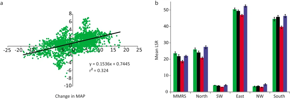
correspond to those scenarios in which the MAP was among the lowest or highest, respectively, for a given system, there Figure 6. (a) Changes in local species richness as given by the model versus changes in mean annual

pre-cipitation. Changes were calculated at the DTA scale for both the species‐poor and species‐rich scenarios for

each system using the model results as the baseline. There is a generally increasing trend between changes in LSR and changes in MAP, indicating that increased values of MAP do tend to lead to an increase in LSR. However, ther2value of the best‐fit line is 0.32, which indicates that MAP is not the sole driver of LSR.

From this graph, we see that, although MAP does influence LSR, so do other factors, such as the spatial heterogeneity of precipitation, landscape connectivity, and dispersal. (b) Impact of climate change on the region‐averaged LSR of each region. Green bars illustrate empirical data, black bars the current climate

sce-nario, red bars the species‐poor scenario, and blue bars the species‐rich scenario. The bars show the means

and the error bars represent the standard deviations of the average LSR estimated across all DTAs in the region. When error bars fall within one another, the differences are not considered statistically significant. The error bars resulting from the model under the current climate are within those of the empirical data for all systems. However, the error bars of the species‐poor scenarios are significantly different from the current

climate model in all systems, while the error bars of the species‐rich scenarios are significantly different only

in the North, East, and Northwest.

Table 3. Mean LSR for Each System Under Each Scenarioa

System Empirical Data Current‐Climate Species‐Poor Species‐Rich

MMRS 23.60 21.87 18.56 21.81

North 25.95 24.13 20.70 27.32

Southwest 4.06 3.83 2.93 4.20 East 50.48 49.42 46.78 52.54

Northwest 3.40 3.58 2.83 4.68

South 44.51 45.82 39.52 46.38

are situations in which this is not the case. For example, in the South subregion, CNRM‐CM3 is classified as the species‐

poor scenario and GFDL‐CM2.0 as the species‐rich scenario,

even though the average MAP is lower under the GFDL‐

CM2.0 model than under the CNRM‐CM3 model.

[33] To further examine the relationship between LSR and MAP, we graphed changes in LSR against changes in MAP (Figure 6a). Here we calculate changes at the DTA scale for both the species‐poor and species‐rich scenarios for each

system using the model results under the current climate as the baseline. Our key reason for including Figure 6a is to illustrate the important drivers of LSR in our neutral model. Specifically, in Figure 6a, we see that MAP does influence LSR, owing to the generally increasing trend between chan-ges in LSR and chanchan-ges in MAP. However, the lowr2value indicates a loose coupling between these two variables. Because of the lowr2value, we infer that other features of the model contribute to changes in LSR, such as the spatial tribution of precipitation, landscape connectivity, and dis-persal. Similarly, Muneepeerakul et al. [2008] found that model features other than runoff explain large‐scale patterns

of freshwater fish biodiversity.

[34] The impact of climate change on the region‐averaged

local species richness (the mean value of LSR averaged across all DTAs within a given subregion) of each region is shown in Figure 6b. This graph provides further support that the model under the current climate accurately reflects the empirical data for each system. Additionally, in all systems, the region‐averaged LSR under the species‐poor scenarios is

statistically different than under the current climate, while region‐averaged LSR under the species‐rich scenarios is

only significantly different from the current climate in the North, East, and Northwest. This further suggests that tree

diversity is more likely to decrease under climate change across the entire MMRS.

[35] Values of region‐averaged LSR are shown in Table 3.

Only those values that are considered statistically significant in Figure 6b should be considered. Note that the region‐

averaged LSR of the MMRS decreases from 21.87 under the current climate model to 18.56 under the species‐poor model.

This represents a decrease of approximately 15% across the entire MMRS.

[36] Spatially explicit estimates of the impact of climate change under the species‐poor scenarios on region‐averaged

local species richness are mapped in Figure 7. There is a decreasing trend in the percentage of species lost from West to East. However, regions west of the 100°W meridian are composed of species‐poor DTAs, while those to the east

encompass species‐rich DTAs, resulting in the increasing

trend from West to East in the absolute loss in mean LSR. The largest decrease in region‐averaged LSR occurs in the South,

with 6.3 species, on average, lost per DTA across the region.

4.

Conclusions

[37] The neutral metacommunity model used here effec-tively reproduces several characteristic patterns of tree diversity in the MMRS simultaneously. It is noteworthy that these results were derived using a single climatic variable (i.e., mean annual precipitation) to represent habitat capacity at large spatial scales. In this model, habitat capacity, the spatial distribution of precipitation, landscape connectivity, and dispersal are important determinants of large‐scale

bio-diversity characteristics. This partly explains why controls on biodiversity vary across spatial scales and geographic loca-tions; hence the different parameter sets for the subregions.

[38] Because the model is able to reproduce several char-acteristic patterns simultaneously, it is most likely capturing some of the important underlying ecological processes, since patterns are indicators of essential underlying processes [Grimm et al., 2005]. Even though ecological research is still necessary on the processes underlying diversity, neutral theory displays clear utility in capturing macroscopic patterns of biodiversity. The fact that a precise understanding of all of the underlying processes is not yet complete should not hin-der our attempts to predict first‐order approximations of these

important environmental changes.

[39] This parsimonious modeling approach allows for pre-dictions of how biodiversity patterns resulting from the basic processes of ecological drift and dispersal will be affected under projected precipitation patterns at large spatial scales. Our results should be viewed as large‐scale complementary

analyses to niche‐based models, which provide information on

specific species. Our analysis suggests that climate change may dramatically alter key tree diversity patterns in the entire MMRS and subregions. We believe this is an important step toward the quantification of the potential impact of climate change on biodiversity, with far‐reaching implications for

conservation biology and resource management.

[40] Acknowledgments. We acknowledge the Program for Climate Model Diagnosis and Intercomparison (PCMDI) and the World Climate Research Program’s (WCRP) Working Group on Coupled Modeling (WGCM) for their roles in making available the WCRP CMIP3 statistically downscaled climate projections. We would also like to thank Patrick Miles of the USFS for his help in obtaining FIA data. M.K. acknowledges the support

Figure 7. Impact of climate change under the species‐

poor scenario on region‐averaged LSR in subregions of the

MMRS. The acronyms are the same as in Figure 4. Shades of green indicate the percentage change in the region‐

averaged LSR under climate change, with dark green indicat-ing a higher percentage lost. The general trend is that a higher percentage of species are lost in the west with a decreasing trend to the east. The change per DTA in region‐averaged LSR under

climate change is indicated for each region by the bold numb-ers. The species‐rich regions east of the 100°W meridian lose

more species, though these species represent a smaller per-centage of species in these regions. The mean LSR in the South is anticipated to decrease by 6.3 species under climate change, the largest loss of all subregions.

KONAR ET AL.: CLIMATE CHANGE IMPACTS ON TREE DIVERSITY W11515 W11515

of the National Science Foundation (NSF) Graduate Research Fellowship Program (GRFP); R.M. and I.R.‐I. acknowledge the support of the James S. McDonnell Foundation (Transport in River Networks: A Complex System Perspective for Biodiversity and Water‐Borne Diseases); E.B. and A.R. acknowledge the support of the ERC advanced grant RINEC 22671.

References

Algar, A. C., H. M. Kharouba, E. R. Young, and J. T. Kerr (2009), Predict-ing the future of species diversity: macroecological theory, climate change, and direct tests of alternative forecasting methods,Ecography,

32, 22–33.

Bertuzzo, E. R., R. Muneepeerakul, H. J. Lynch, W. F. Fagan, I. Rodriguez‐ Iturbe, and A. Rinaldo (2009), On the geographic range of freshwater fish in river basins, Water Resour. Res., 45, W11420, doi:10.1029/ 2009WR007997.

Botkin, D. B., et al. (2007), Forecasting the effects of global warming on biodiversity,BioScience,57(3), 227–236.

Clark, J. S., et al. (2001), Ecological forecasts: An emerging imperative,

Science,293, 657–660.

Clauset, A. (2010), A theoretician ponders what physics has to offer ecol-ogy,Nature,465(13), 139.

Crawley, M. J., and J. E. Harral (2001), Scale dependence in plant biodi-versity,Science,291, 864–868.

Currie, D. J. (1991), Energy and large‐scale patterns of animal and plant species richness,Am. Nat.,137(1), 27–49.

Dingman, S. L. (2002),Physical Hydrology, 2nd ed., Prentice‐Hall, Englewood Cliffs, N. J.

Fitzpatrick, M. C., and W. W. Hargrove (2009), The projection of species distribution models and the problem of non‐analog climate,Biodiv. Conserv.,

18, 2255–2261.

Grimm, V., E. Revilla, U. Berger, F. Jeltsch, W. M. Mooij, S. F. Railsback, H.‐H. Thulke, J. Weiner, T. Wiegand, and D. L. DeAngelis (2005), Pattern‐ oriented modeling of agent‐based complex systems: lessons from ecology, Science,310, 987–991.

Guisan, A., and W. Thuiller (2005), Predicting species distribution: Offer-ing more than simple habitat models,Ecol. Lett.,8, 993–1009. Hubbell, S. P. (2001),The Unified Neutral Theory of Biodiversity and

Biogeography, Princeton Univ. Press, Princeton, N. J.

Hui, C. (2009), On the scaling patterns of species spatial distribution and association,J. Theor. Biol.,261, 481–487.

Ibanez, I., J. S. Clark, M. C. Dietz, K. Feeley, M. Hersh, S. LaDeau, A. McBride, N. E. Welch, and M. S. Wolosin (2006), Predicting bio-diversity change: Outside the climate envelope, beyond the species‐area curve,Ecology,87(8), 1896–1906.

Intergovernmental Panel on Climate Change (2007),Climate Change 2007: The Physical Science Basis. Contribution of Working Group I to the Fourth Assessment Report of the Intergovernmental Panel on Climate Change, edited by S. Solomon et al., Cambridge Univ. Press, Cam-bridge, U. K.

Jeltsch, F., K. A. Moloney, F. M. Schurr, M. Kochy, and M. Schwager (2008), The state of plant population modelling in light of environmental change,Persp. Plant Ecol., Evol. and System.,9, 171–189.

Karl, T. R., J. M. Melillo, and T. C. Peterson (2009),Global Climate Change Impacts in the United States, Cambridge Univ. Press,

Cam-bridge, U. K.

McGill, B. J. (2010), Matters of scale,Ecology,328, 575–576.

Millenium Ecosystem Assessment (2005),Ecosystems and Human Well‐

Being: Current State and Trends, vol. 1, Island, Washington, D. C. Morin, X., and W. Thuiller (2009), Comparing niche‐and process‐based

models to reduce prediction uncertainty in species range shifts under cli-mate change,Ecology,90(5), 1301–1313.

Muneepeerakul, R., E. Bertuzzo, H. J. Lynch, W. F. Fagan, A. Rinaldo, and I. Rodriguez‐Iturbe (2008), Neutral metacommunity models predict fish diversity patterns in Mississippi‐Missouri basin,Nature,453, 220–222. National Hydrography Dataset (2008), NHD Plus Data, http://www.

horizon‐systems.com/nhdplus/index.php, Herndon, Va.

O’Dwyer, J. P., and J. L. Green (2010), Field theory for biogeography: A spatially explicit model for predicting patterns of biodiversity,Ecol. Lett.,13, 87–95.

Pearson, R. G., and T. P. Dawson (2003), Predicting the impacts of climate change on the distribution of species: Are bioclimate envelope models useful?,Global Ecol. Biogeogr.,12, 361–371.

Rockström, J., et al. (2009), A safe operating space for humanity,Nature,

461, 472–475.

Rodriguez‐Iturbe, I., V. K. Gupta, and E. Waymire (1984), Scale consider-ation in the modeling of temporal rainfall,Water Resour. Res.,20(11), 1611–1619, doi:10.1029/WR020i011p01611.

Rosenzweig, M. L. (1995),Species Diversity in Space and Time, Cam-bridge Univ. Press, CamCam-bridge, U. K.

Sala, O. E., et al. (2000), Global biodiversity scenarios for the year 2100,

Science,287, 1770–1774.

Sankaran, M., et al. (2005), Determinants of woody cover in African savan-nas,Nature,438(8), 846–849.

Thuiller, W., et al. (2008), Predicting global change impacts on plant spe-cies’distributions: Future challenges,Persp. Plant Ecol., Evol. System.,9,

137–152.

U.S. Forest Service (2008), FIA Data Mart 4.0, http://199.128.173.17/ fiadb4‐downloads/datamart.html.

Walther, G.‐R., E. Post, P. Convey, A. Menzel, C. Parmesan, T. J. C. Beebee, J.‐M. Fromentin, O. Hoegh‐Guldberg, and F. Bairlein (2002), Ecological responses to recent climate change,Nature,416(28), 389–395.

S. Azaele, M. Konar, R. Muneepeerakul, and I. Rodriguez‐Iturbe, Department of Civil and Environmental Engineering, Princeton University, Engineering Quad, Princeton, NJ 08544, USA. (sazaele@princeton.edu; mkonar@princeton.edu; rmuneepe@princeton.edu; irodrigu@princeton. edu)