Limit analysis of plates using the EFG method and second-order cone programming

White Rose Research Online

[email protected]

Universities of Leeds, Sheffield and York

http://eprints.whiterose.ac.uk/

This is an author produced, pre-peer review version of a paper published in

International Journal for Numerical Methods in Engineering

.

White Rose Research Online URL for this paper:

http://eprints.whiterose.ac.uk/10835/

Published paper

Le, Canh V., Gilbert, Matthew and Askes, Harm (2009)

Limit analysis of plates

using the EFG method and second-order cone programming.

International

Journal for Numerical Methods in Engineering, 78 (13). pp. 1532-1552.

second-order cone programming

Canh V. Le, Matthew Gilbert, Harm Askes

Department of Civil and Structural Engineering, The University of Sheffield, United Kingdom

SUMMARY

The meshless Element-Free Galerkin (EFG) method is extended to allow computation of the limit load of plates. A kinematic formulation which involves approximating the displacement/velocity field using the moving least squares technique is developed. Only one displacement variable is required for each EFG node, ensuring that the total number of variables in the resulting optimization problem is kept to a minimum, with far fewer variables being required compared with finite element formulations. A stabilized conforming nodal integration scheme is extended to plastic plate bending problems. The evaluation of integrals at nodal points using curvature smoothing stabilization both keeps the size of the optimization problem small and also results in stable and accurate solutions. Difficulties imposing essential boundary conditions are overcome by enforcing directly displacements at the nodes. The formulation can be expressed as the problem of minimizing a sum of Euclidean norms subject to a set of equality constraints. This non-smooth minimization problem can be transformed into a form suitable for solution using Second-Order Cone Programming (SOCP). The procedure is applied to several benchmark problems and is found in practice to generate good upper bound solutions for benchmark problems. Copyright c2008 John Wiley & Sons, Ltd.

key words: Limit analysis, EFG method, nodal integration, second order cone programming

1. INTRODUCTION

Limit state criteria are applied to the safety assessment and design of many engineering structures. Considering the ultimate limit state, a traditional and popular approach is to perform a complete elastoplastic analysis. However, an elastoplastic analysis procedure tends to be quite complex due to the need carry this out in an iterative and incremental manner. Alternatively, by applying the fundamental theorems of plasticity, limit analysis can be used to directly identify upper and lower bounds on the load multiplier at collapse, without intermediate steps. There has been a resurgence in interest in computational limit analysis procedures in recent years, principally thanks to the availability of highly efficient optimization algorithms, which have developed rapidly.

∗_{Correspondence to: Harm Askes, Department of Civil and Structural Engineering, University of Sheffield,}

Computational limit analysis generally involves two steps: (i) numerical discretisation; and (ii) mathematical programming to enable a solution to be obtained. Computational limit analysis approaches based on the finite element method (FEM) are well-established. Significant contributions include [1–4]. Once the stress or displacement/velocity fields are approximated and the bound theorems applied, limit analysis becomes a problem of optimization involving either linear or nonlinear programming. While linear programming involves piecewise linear yield functions, nonlinear programming involves nonlinear yield surfaces. Much progress has been made in developing numerical procedures for limit analysis problems [5–10]. Current research is focussing on developing limit analysis tools which are sufficiently efficient and robust to be of use to engineers working in practice. However, when FEM is applied some of the well-known characteristics of mesh-based methods can lead to problems: the solutions are often highly sensitive to the geometry of the original mesh, particularly in the region of stress or displacement/velocity singularities; furthermore, volumetric locking may occur in plane strain and 3D problems [11]. Although adaptive schemes with the h-version [12–16] or p-version FEM [17, 18] have been used to try to overcome such disadvantages, and show immense promise, the schemes quickly become complex and a large number of elements are generally required to obtain accurate solutions. On the other hand, the objective function in the associated optimization problem is convex, but not everywhere differentiable. One of the most efficient algorithms to overcome this difficulty is the primal-dual interior-point method presented in [19,20] and implemented in commercial codes such as the Mosek software package. The limit analysis problem involving conic constraints can then be solved by this efficient algorithm [16, 21, 22].

In recent years so-called ‘meshless’ methods have been developed to provide a flexible alternative approach to FEM. The methods use sets of nodes distributed across the problem domain, and also along domain boundaries. One of the first meshless methods developed is the Element-Free Galerkin (EFG) method [23]. The EFG method has been applied successfully to a wide range of computational problems, proving popular due to its rapid convergence characteristics and its ability to obtain highly accurate solutions for problems involving stress discontinuities and/or for problems prone to volumetric locking when using FEM [23–25]. It therefore seems appropriate to investigate the performance of the EFG method when applied to limit analysis problems. Recently, a numerical procedure for lower-bound limit analysis was presented by [26]. In the paper, a self-equilibrium stress basis vector at each Gaussian point is computed using the EFG method. Although this does not guarantee a strict lower-bound, a reliable estimate of the limit load factor can be obtained when the discretisation is sufficiently fine. It is shown that the achieved solution of 2D problems are in good agreement with other solutions.

In this paper a numerical procedure based on the EFG method for upper-bound limit analysis of rigid-perfectly plastic plates governed by the von Mises criterion is proposed. Nodal collocation is used to impose essential boundary conditions. A stabilized conforming nodal integration (SCNI) scheme is used to evaluate the integral of both internal dissipation power and work rate of external load. This results in a truly meshless method and reduces computational effort. Attention is also focused on formulating the plate limit analysis problem as one of minimizing a sum of Euclidean vector norms, which can be solved efficiently by a primal-dual interior-point method [19], such as Second-Order Cone Programming (SOCP). To illustrate the method it is then applied to a series of bending problems, including those for which solutions already exist in the literature.

Copyright c2008 John Wiley & Sons, Ltd. Int. J. Numer. Meth. Engng2008;0:0–0

2. LIMIT ANALYSIS OF PLATES - KINEMATIC FORMULATION

Consider a rigid-perfectly plastic plate subjected to surface traction αf on the free portion Γt of its boundary and constrained boundary Γu. According to Kirchhoff’s hypothesis, if w

denotes the transverse displacement, the strain rates can be expressed by relations

˙

=zκ˙ (1)

with the vectors of strains and curvatures

˙

= ˙xx ˙yy γ˙xy

T

(2)

˙

κ=∇2_{w˙ =}n ∂2w˙

∂x2 ∂ 2_˙

w

∂y2 2∂ 2_˙

w

∂x∂y

oT

(3)

In framework of a limit analysis problem, only plastic strains are considered and are assumed to obey the normality rule

˙

= ˙λ∂Φ

∂σ (4)

where the plastic multiplier ˙λ is non-negative and the yield function Φ(σ) is convex. In this study, the von Mises failure criterion is used

Φ(σ) =√σT _Pσ−σ

0≤0 (5)

where σ0 is the yield stress and

σ= σxx σyy τxy T (6)

P= 1 2



 ₋21 −21 00 0 0 6



 (7)

The plastic dissipation is expressed by

Dp = max(σ∗) =σ (8)

where σ∗ represents the admissible stresses contained within the convex yield surface and

σ represents the stresses on the yield surface associated to any strain rates ˙ through the plasticity condition. Since the stress space described in Eq. (5) is bounded in all directions, any strain rate is normal to its boundary and no constraints are introduced. Then the power of dissipation can be formulated as a function of strain rates as

Dp(σ, ) =σ0

p ˙

T_{Q˙ (9)}

where

Q=P−1₌ 1

3 

 4 2 02 4 0 0 0 1



 (10)

The internal dissipation power of the two-dimensional plate domain Ω can be written as

˙

Wint( ˙κ) =

Z

Ω t/2

Z

−t/2

Dp(σ, ) dΩ =mp

Z

Ω

p ˙

where mp=σ0t2/4 is the plastic moment of resistance of a plate of thicknesst.

The upper bound limit analysis problem for plates can be expressed as

α+= min ˙Wint( ˙κ) (12)

subject to

˙

κ=_∇2w˙ (13)

˙

Wext=

Z

Ω

q ˙wdΩ = 1, u˙ = ˙ˉu on Γu (14)

whereα+_{is the load factor and where Eq. (14) represents unitary external work and boundary}

conditions, respectively.

3. THE EFG METHOD

The moving least square technique is utilized to construct an approximation function uh_(x)

that fits a discrete set of data so that [23]

uh(x) =

n

X

I=1

ΦI(x)uI (15)

ΦI(x) =pT(x)A−1(x)BI(x) (16)

A(x) =

n

X

I=1

wI(x)pT(xI)p(xI) (17)

BI(x) =wI(x)p(xI) (18)

where nis the number of discretized nodes; p(x) is a set of basis function; wI(x) is a weight function associated with node I. For the purpose of consistency of fourth-order problems, the polynomial basis function p(x) must be at least quadratic [27]. In this work, the quadratic polynomial for 2D bending problems is used, which is given by

pT(x) = 1, x, y, xy, x2, y2 (19)

Furthermore, for the weight functions an isotropic quartic spline function is used, i.e.

wI(x) =

1₋6s2_{+ 8s}3

−3s4 _ifs ≤1

0 ifs >1 (20)

withs= kx−xIk

Ri ,whereRi is the support radius of nodei. We will need first and second order

partial derivatives of the shape function with respect to x.

To avoid the loss of accuracy due to roundoff error the origin is shifted to the evaluation point. The argument x should be replaced by a simple linear transformation ˉx =x₋xorig,

[28].

Copyright c2008 John Wiley & Sons, Ltd. Int. J. Numer. Meth. Engng2008;0:0–0

4. STABILIZED CONFORMING NODAL INTEGRATION

The integrals in Eqs. (11, 14) are commonly evaluated by Gauss integration which requires the use of background integration cells. It is normal to use rectangular and triangle cells and high order quadratures. As an alternative, nodal integration which uses nodes as integration points is employed. This results in a truly meshless method due to the absence of integration cells. However, direct nodal integration is instable because of under integration and vanishing derivatives of shape functions at the nodes [29]. A stabilized conforming nodal integration (SCNI) is proposed in [30] to eliminate spatial instability problems and to improve accuracy and convergence properties. The main idea of the method is that nodal strains are determined by spatially averaging strains using the divergence theorem. We will extend this idea here to plastic plate bending.

With the use of nodal integration and strain smoothing stabilization, Eq. (11) yields

˙

Wint=mp n

X

j=1 aj

q

κT_(x

j)Qκ(xj) (21)

in which κ(xj) follows from curvature smoothing at nodal point xj [31, 32]

κT(xj) =−

Z

Ωj

[ ˙w,xx, w˙,yy, 2 ˙w,xy] dΩ

=−

I

Γj

[ ˙w,xnx, w˙,yny, ( ˙w,xny + ˙w,ynx)] dΓ (22)

where Ωj is the nodal representative domain that can be a Voronoi diagram;aj and Γj are its

area and boundary, respectively.

Introducing a moving least square approximation of the transverse displacement w(x), the smoothed curvatureκ(xj) is expressed as

κT(xj) =−

n

X

I=1

˜

∇ΦI,(xj)uI =−G d (23)

dT = [ ˙u1, u˙2, . . . ,u˙n] (24)

G=h_∇˜Φ1,(xj), ∇˜Φ2,(xj), . . . ,∇˜Φn,(xj)

i

(25)

˜

∇T_Φ

I,(xj) =

1

aj

I

Γj

[ΦI,x(xj)nx, ΦI,y(xj)ny, (ΦI,x(xj)ny+ΦI,y(xj)nx)] dΓ (26)

In order to evaluate components in Eq. (26), there is a need to perform a boundary integration of the representative nodal domain. The calculation of these components is given by

1

aj

I

Γj

ΦI,x(xj)nxdΓ =

1 2aj

ns

X

k=1

nkxlk+nkx+1lk+1

ΦI,x(xk+1) (27)

1

aj

I

Γj

ΦI,y(xj)ny dΓ =

1 2aj

ns

X

k=1

nky lk+nky+1lk+1

1

aj

I

Γj

(ΦI,x(xj)ny+ΦI,y(xj)nx) dΓ = 1

2aj ns

X

k=1

nky lk+nky+1lk+1ΦI,x(xk+1)

+ 1 2aj

ns

X

k=1

nkxlk+nkx+1lk+1ΦI,y(xk+1) (29)

where ns is the number of segments of a Voronoi nodal domain, as shown in Figure 1; xk

and xk+1 are coordinates the two end points of boundary segmentk which has lengthlk and

outward surface normalnk_{. Note that the Voronoi node numberskare defined recursively, i.e.}

k=ns+ 1→k= 1.

j Γ1 j 1 Γns j 1 Ωj 1 Γk j 1 xk j 1

xk+1

j 1 lk 1 nk 1

Figure 1. Geometry definition of a representative nodal domain

Similarly, the external energy can be determined using a nodal integration scheme and moving least square approximation of the transverse displacementw(x) as

˙

Wext =

Z

Ω

q ˙wdΩ =

n

X

j=1

ajqw˙(xj)

= n X j=1 n X I=1

ajqΦI(xj) ˙uI (30)

Hence the upper bound limit analysis problem for plates can be formulated as

α+= min mp n

X

j=1 aj

q

κT_(x

j)Qκ(xj)

Subject to n X j=1 n X I=1

ajqΦI(xj) ˙uI = 1, u˙ = ˙ˉu on Γu (31)

Considering boundary conditions, it is important to note that enforcement of ˙uI = ˙ˉuI is not

appropriate since the moving least square does not satisfy the Kronecker delta property and

Copyright c2008 John Wiley & Sons, Ltd. Int. J. Numer. Meth. Engng2008;0:0–0

therefore ˙uI is not the velocity at nodeI. To overcome this difficulty, collocation at nodes [33]

is used to enforce essential boundary conditions: ˙uh_(x

b) = ˙ˉuI(xb), xb are nodes on essential

boundaries. Since essential boundaries are fixed, the boundary conditions are given as

˙

w(xb) = n

X

I=1

ΦI(xb) ˙uI = 0 (32)

˙

θx= ˙wx(xb) =

n

X

I=1

ΦI,x(xb) ˙uI = 0 (33)

˙

θy= ˙wy(xb) =

n

X

I=1

ΦI,y(xb) ˙uI = 0 (34)

Where Eq. (32), (33) and (34) enforce the vertical deflection and x and y axis rotations respectively. Then Eq. (31) can be written as a standard linear equality constraint

Aeqd=beq (35)

where the matrix Aeq and vectorbeq of Eq. 35 are given by

Aeq =

                     n P j=1

ajΦ1(xj) n

P

j=1

ajΦ2(xj) . . .

n

P

j=1

ajΦn(xj)

Φ1(xb1) Φ2(xb1) . . . Φn(xb1)

..

. ... . .. ...

Φ1(xbd) Φ2(xbd) . . . Φn(xbd)

Φ1,x(xb1) Φ2,x(xb1) . . . Φn,x(xb1)

..

. ... . .. ...

Φ1,x(xbrx) Φ2,x(xbrx) . . . Φn,x(xbrx)

Φ1,y(xb1) Φ2,y(xb1) . . . Φn,y(xb1)

..

. ... . .. ...

Φ1,y(xbry) Φ2,y(xbry) . . . Φn,y(xbry)

                     (36) bT eq= " 1 d

z }| {

0 0 . . . 0

rx

z }| {

0 0 . . . 0

ry

z }| {

0 0 . . . 0

#

(37)

d is the number of boundary nodes having deflection conditions, rx, ry is the number of boundary nodes having rotation conditions aboutxandy, respectively. .

5. SECOND-ORDER CONE PROGRAMMING

problem of this sort can be cast as a Second-Order Cone Programming (SOCP) problem, for which highly efficient solvers exist. Further details of SOCP and its applications can be found in [35]; the general form of an SOCP problem is as follows

min fTx

Subject to _kHix+vik ≤yiTx+zi (38)

where x _∈ Rn _{are the optimization variables, and the problem coefficients are f}

∈ Rn_,

Hi ∈ Rm×n, vi ∈ Rm, yi ∈ Rn, and zi ∈ R. For optimization problems in 2D or 3D

Euclidean space, m = 2 or m = 3. When m = 1 the SOCP problem reduces to a linear programming problem.

Since Qin Eq. (21) is a positive definite matrix, this can be rewritten in a form involving a sum of norms as

˙

Wint=mp n

X

j=1

ajkCT κ(xj)k=mp n

X

j=1

ajkCTGdk (39)

where Cis the so-called Cholesky factor ofQ

C=√1

3  

2 0 0 1 √3 0 0 0 1



 (40)

Note that Cdepends only on the yield condition; for one-dimensional problems C= 1. The upper bound limit analysis of plates problem can be now written as one of minimizing a sum of norms subject to linear equality constraints

α+= min mp n

X

j=1

ajkCTGdk

Subject to Aeqd=beq (41)

This is a convex programming problem in which the objective function is not differentiable at any point in the rigid domain where plastic strains do not develop (CT_{Gd= 0). Of the}

several methods that have been developed to treat such a singularity, the primal-dual interior-point method proposed by Andersen et. al [19] has been found to be especially efficient. The traditional way of replacing the singular function by a differentiable one is to add a square of a fixed positive number μ to the root, so that the function becomes pkCT_Gdk2_+μ2_.

However, this may lead to slow convergence as μ_→0. In [19], the quantityμis treated as an additional variable and can be determined by a duality estimate. With the use of this method, the optimization problem is solved rapidly and accurately even if there are a large number of variables and/or zero terms in the objective function. Since the method is implemented in generally available second order cone programming software (e.g. Mosek), the limit analysis problem can be efficiently solved using such software.

Thus the present optimization problem is cast as a standard SOCP problem by introducing auxiliary variables t1, t1, . . . , tn

α+= min mp n

X

j=1 ajtj

Copyright c2008 John Wiley & Sons, Ltd. Int. J. Numer. Meth. Engng2008;0:0–0

Subject to Aeqd=beq; CTGd=ri (42)

krik≤ti, i= 1,2, . . . , n (43)

in which Eq. (41) expresses quadratic cones and ri ∈ Rn are additional variables defined by

Eq. (40), where every ri is a 3×1 vector.

6. NUMERICAL EXAMPLES

The numerical performance of the method is illustrated by applying it to uniformly loaded plate problems for which, in most cases, solutions already exist in the literature (the method is applicable to problems of arbitrary geometry). For all the examples considered the following was assumed: lengthL= 10 m; plate thicknesst= 0.1 m; yield stressσ0= 250 MPa. Quarter

symmetry was assumed when appropriate (see Figure 2).

Figure 2. Square plate clamped along edges and loaded by a uniformly pressure

The radius of influence domainRi at nodeith is determined by

Ri=dmaxhi (44)

where dmax and hi are the dimensionless size of influence domain and the nodal spacing,

respectively (Figure 3).

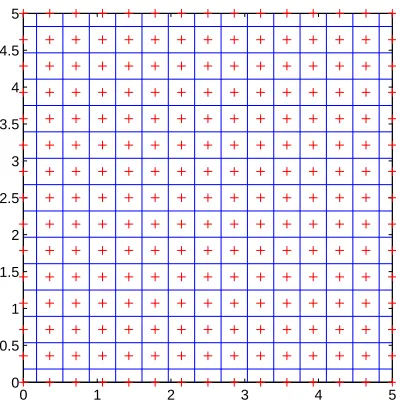
The example comprises a square plate with clamped supports and subjected to uniform out-of-plane pressure loading. A uniform discretisation n= 15_×15 nodes (Figure 4) and various sizes of influence domaindmax= 3∼9 were used. Matlab optimization toolbox 3.0 and Mosek

Figure 3. Sizes of influence domain

0 1 2 3 4 5

0 0.5 1 1.5 2 2.5 3 3.5 4 4.5 5

Figure 4. Nodes (15_×15) and geometry definition of Voronoi diagram

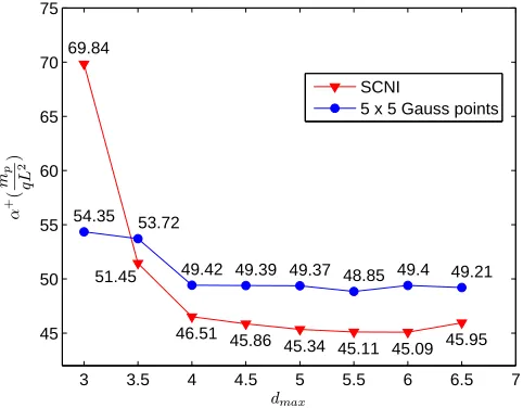
Firstly, potential integration schemes were considered. In the formulation presented a quadratic basis function and an isotropic quartic spline weight function were used with a moving least squares approximation, which results in a high order of approximated displacement field. Therefore, in order to evaluate accurately the integrals in the limit analysis problem, very large numbers of Gauss points would be needed. Here results are reported for the plate problem with 5_×5 Gauss points per cell. It can be seen in Figure 5 that the

Copyright c2008 John Wiley & Sons, Ltd. Int. J. Numer. Meth. Engng2008;0:0–0

solutions obtained using SCNI are lower, and hence likely to be more accurate, than when using 5×5 Gauss points (except for the extreme case of dmax = 3). i.e. SCNI appears to increase the accuracy of solutions as long as the radius of the influence domain is sufficiently large. If nonlinear programming is employed both SCNI and Gauss integration schemes give rise to problems with an identical number of variables (equal to the number of discretisation nodes, n= 225 in this case). However, less CPU time is required to evaluate integrals when using the SCNI scheme. The difference in CPU time is even more marked when either linear programming or SOCP are used to solve the underlying optimization problem. This is because additional variables need to be added, a total of 5nwhen Gauss integration is used compared withnwhen SCNI is used. In summary, SCNI appears to offer a good combination of accuracy and computational efficiency, not only for elastic analysis problems [30] but now also for plastic analysis problems.

3 3.5 4 4.5 5 5.5 6 6.5 7

45 50 55 60 65 70 75

α

+(

mp qL

2

)

1

dmax

69.84

51.45

46.51 45.86 _{45.34 45.11 45.09} 45.95 54.35 _53.72

49.42 49.39 49.37 48.85 49.4 49.21 SCNI

5 x 5 Gauss points

Figure 5. Limit load factor for various influence domain sizes

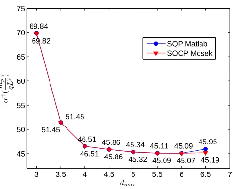
Next, the efficacy of various optimization algorithms was considered (using SCNI). Figure 6 shows that SQP and SOCP algorithms produced very similar solutions for the square plate problem. However, the SOCP algorithm produced solutions very much more quickly, even though the number of variables involved was much greater (5n cf. n when using SQP). The SOCP algorithm typically took only 2∼5 s to compute a solution, compared with 300∼600 s using SQP. Moreover, the SOCP algorithm can be guaranteed to identify globally optimal solutions, whereas SQP cannot.

It is advantageous to choose a size of influence domain that meets both accuracy and computation cost requirements. With this in mind, the radius of influence domain was set to be equal to 6hi for all plate problems, although the result of a higher radius value may be a better upper-bound. Solutions obtained with Ri= 6hiare used for comparison with other’s

in all tables.

Table I compares the solution obtained using the present solution with previously obtained solutions obtained using FEM simulations. In comparison with the other upper bound

Copyright c2008 John Wiley & Sons, Ltd. Int. J. Numer. Meth. Engng2008;0:0–0

LIMIT ANALYSIS OF PLATES 11

3 3.5 4 4.5 5 5.5 6 6.5 7

45 50 55 60 65 70 75

α

+(

mp qL

2

)

dmax

1

69.84

51.45

46.51 45.86 _{45.34 45.11 45.09} 45.95 69.82

51.45

46.51 45.86 _{45.32 45.09 45.07 45.19} SQP Matlab SOCP Mosek

Figure 6. Comparison between SQP and SOCP using SCNI

solutions, the present result is lower than solutions in [36], [1] and [34] by 13.34%, 8.49% and 0.49% respectively. If a comparison is made in terms of the number of variables in the optimization problem, the present method using EFG has a significantly smaller number than mesh-based approaches; in the EFG method there is only one variable at each node while at least 3 are required when FEM is used (deflection and 2 rotation components) [34]. The only obvious drawback is that the high order shape functions used in EFG make a priori proof of the strict upper bound status of the solutions difficult (though these can potentially be checked

a posteriori).

Table I. Limit load factor of clamped plate in comparison with other solutions

Authors upper bound lower bound (_qLmp2)

Present method 45.07+ _–

Hodge and Belytschko [1] 49.25 42.86

Lubliner [36] 52.01 –

Capsoni and Corradi [34] 45.29 –

Andersen et al. (mixed element) [10] 44.13

+_{Approximate rather than rigorous upper bound due to the high order EFG shape functions used}

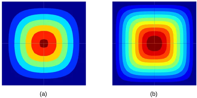
Further illustration of the method can be made by examining the same square plate with different boundary conditions. Table II provides solutions in the case of a uniformly loaded square plate with simply supported edges. The limit load factor obtained by the proposed method is the lowest. Figure 7 shows the associated collapse mechanisms for both clamped and simply supported plates.

Rectangular plates (dimensions a_×b) with different boundary conditions under uniform pressure were also considered. Collapse mechanisms and limit loads are shown in Figure 8 and Table III, with a_÷b= 2. The plate with 3 clamped and 1 free edge was solved using 60_×15

Copyright c2008 John Wiley & Sons, Ltd. Int. J. Numer. Meth. Engng2008;0:0–0

(a) (b)

Figure 7. Iso-displacement contours at collapse for uniformly loaded plates: (a) clamped; (b) simply supported

Table II. Limit load factor of simply supported plate in comparison with other solutions

Authors upper bound lower bound (_qLmp2)

Present method 25.01+ _–

Hodge and Belytschko [1] 26.54 24.86

Lubliner [36] 27.71 23.81

Capsoni and Corradi [34] 25.02 –

Andersen et al. (mixed element) [10] 25.00

+_{Approximate rather than rigorous upper bound due to the high order EFG shape functions used}

nodes using half symmetry whilst in the remaining cases quarter symmetry was used with 30_×15 nodes. It is evident from Table III that the present solution for the simply supported case is in excellent agreement to the solution obtained in [34]. It should also be noted that plates having simply supported boundaries converge faster than those with clamped boundaries (see Figure 9).

Table III. Collapse limit load of rectangular plates with various boundary conditions

Models clamped supported 3 clamped, 1 free 2 clamped, 2 free (mp_qab) Present results 54.61 29.88 43.86 9.49

Capsoni et at. [34] – 29.88 – –

(a) (b)

(c) (d)

Figure 8. Iso-displacement contours at collapse for uniformly loaded rectangular plates: (a) clamped plate (b) simply supported (c) 3 clamped edges, 1 free (d) 2 clamped, 2 free edges

200 300 400 500 600 700 800 900 1000

0 10 20 30 40 50 60 70

59.88

30.11 49.15

9.78

57.83

29.99 46.79

9.59

55.94

29.91 45.57

9.52

54.61

29.88 43.86

9.49

α

+ (

mp qab

)

1

number of nodes (n) clamped plate simply supported 3 clamped - 1 free 2 clamped - 2 free

Figure 9. Collapse multipliers for rectangular plates

7. CONCLUSIONS

The numerical implementation of limit analysis problems using the Element-Free Galerkin (EFG) method and mathematical programming has been investigated. The numerical procedure demonstrates that the EFG method can be applied successfully not only to

lower-Copyright c2008 John Wiley & Sons, Ltd. Int. J. Numer. Meth. Engng2008;0:0–0

Figure 10. L-shaped geometry

Figure 11. Iso-displacement contours at collapse for uniformly loaded L-shaped plate

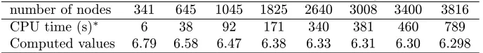
Table IV. Collapse limit load of L-shape plateα+₍mp

qL2)

number of nodes 341 645 1045 1825 2640 3008 3400 3816 CPU time (s)∗ 6 38 92 171 340 381 460 789 Computed values 6.79 6.58 6.47 6.38 6.33 6.31 6.30 6.298

bound limit analysis problems [26] but also to upper-bound limit analysis problems. The solutions obtained show good agreement with results available in the literature. Advantages of applying EFG to limit analysis problems are that problem size is reduced, and accurate solutions can be obtained using a relatively small number of nodes. The combination of the stabilized conforming nodal integration technique (SCNI) and second order cone programming (SOCP) optimization algorithm leads to an efficient and robust method. The main features of the method can be summarized as:

1. Since the displacement field is approximated using the moving least squares technique, the problem field and its derivatives are smooth across the whole domain. Due to the use of only one nodal parameter (displacement only rather than displacement and two rotations) the number of variables in the optimization problem is small compared with the number required in finite element method formulations.

2. The SCNI scheme has been applied successfully to the kinematic limit analysis of plates problem. The SCNI scheme results in a truly meshless method and stable solutions. This nodal integration scheme produces more accurate results than when Gauss integration is used. Furthermore, the size of optimization problem reduces significantly when this smoothing technique is used in conjunction with the Element-Free Galerkin method. 3. A primal-dual interior-point SOCP algorithm can efficiently solve problems involving

linear or conic constraints. This algorithm is of particular interest in the field of limit analysis since most plasticity problems can be formulated as conic programming problems [22].

Finally, although a kinematic limit analysis formulation for plates is presented here, the numerical procedure can be extended to tackle more complex structural configurations, subject to a variety of loading regimes. It would for example be interesting to extend the proposed method to treat plane strain problems, 3D problems and also problems involving shakedown.

ACKNOWLEDGEMENTS

This research has been sponsored by the Ho Chi Minh City Government (300 Masters & Doctors Project) and the University of Sheffield.

APPENDIX

I. Beam bending example

Since the Euler beam is the one dimensional degeneration of the Kirchhoff plate, limit analysis of beams in bending can be considered to examine the effectiveness of the proposed method in a lower dimension. Beams of rectangular cross section (b×h) are subjected to a uniform load and various boundary conditions at the ends, as shown in Figure 12. Analytical limit load factors for beams are given as

λ+= mp

qL2

  

16.000 beam clamped at ends

11.657 clamped-simply supported beam 8.000 beam simply supported at ends

(45)

wheremp=σ0bh2/4 is the plastic moment of beams.

Copyright c2008 John Wiley & Sons, Ltd. Int. J. Numer. Meth. Engng2008;0:0–0

Figure 12. Clamped beam subjected to uniform load

The kinematic formulation of the beam problem is the reduced form of the kinematic plate limit analysis problem, in which the curvature component is κx = ˙w,xx only and C = 1. The smoothed

curvature at node jth_{on beam can be calculated as} κ(xj) = 1

Δxj(ΦI,x(xjR)−Φ,x(xjL)) (46)

where Δxj=xjR−xjLis the length of representative length Ωj, as shown in Figure 13.

Figure 13. Degeneration of Voronoi diagram to one-dimension

The limit analysis of beams problem is one which can be solved by linear programming, or alternatively using a SOCP algorithm. Therefore, most of the techniques used in plate problems can be applied here for beams.

Half symmetry was used when possible, with 81 and 161 nodes used to discretize the simply supported and clamped beams respectively. The beam clamped at one end and simply supported at the other was modelled in full, using a total of 321 nodes.

As can be seen from Figure 14, taking dmax = 3.5hi appears to give the best results. Limit load

factors are reported in Table V and it can be seen that the numerical results are in good agreement with analytical solutions. This demonstrates the efficiency and high accuracy of proposed numerical procedure when applied to one-dimensional problems.

The convergence rates are plotted in Figure 15. They range between the theoretically expected value of 1 : 1 for the clamped beam to 1 : 2 for the simply supported beam; see Figure 15.

Table V. Collapse limit load of beams in comparison with analytical solutions (mp

qL2)

Present method Analytical solution error (%)

Clamped 16.051 16.000 0.31

Simply supported (s.s) 8.001 8.000 _∼0.00 1 clamped, 1 s.s 11.666 11.657 0.08

LIMIT ANALYSIS OF PLATES 17

3 3.5 4 4.5 5 5.5 6 6.5

8 10 12 14 16

Clamped beam

Simply supported beam Clamped-simply supported beam

α

+(

mp qL

2

)

dmax

1

SCNI

Gauss integration Analytical solution

Figure 14. Comparison of Gauss integration and SCNI for 1-D problems

0.5 1 1.5 2 2.5 3 3.5

-2.5 -2 -1.5 -1 -0.5 0 0.5

1 1

1 2

Log

10

(Error in Load Factor)

Log 10 (n) clamped beam

simply supported clamped-simply supported

Figure 15. Rate of convergence for beam problems

1. P. G. Hodge and T. Belytschko. Numerical Methods for the Limit Analysis of Plates. Applied Mechanics, 35:796–801, 1968.

2. H. D. Nguyen. Direct limit analysis via rigid-plastic finite elements. Computer Methods in Applied Mechanics and Engineering, 8:81–116, 1976.

3. A. Capsoni and L. Corradi. A finite element formulation of the rigid-plastic limit analysis problem. Int. J. Numer. Meth. Engng., 40:2063–2086, 1997.

4. E. Christiansen and K. D. Andersen. Computation of collapse states with von Mises type yield condition.

International Journal for Numerical Methods in Engineering, 46:1185–1202, 1999.

5. V. F. Gaudrat. A Newton type algorithm for plastic limit analysis. Computer Methods in Applied Mechanics and Engineering, 88:207–224, 1991.

Copyright c2008 John Wiley & Sons, Ltd. Int. J. Numer. Meth. Engng2008;0:0–0

6. N. Zouain, J. Herskovits, L. A. Borges, and R. A. Feijo. An iterative algorithm for limit analysis with nonlinear yield functions. International Journal of Solids and Structures, 30:1397–1417, 1993.

7. Y. H. Liu, Z. Z. Zen, and B. Y. Xu. A numerical method for plastic limit analysis of 3-D structures.

International Journal of Solids Structures, 32:1645–1658, 1995.

8. E. Christiansen and K. O. Kortanek. Computionion of the collapse state in limit analysis using the LP affine scaling algorithm. Journal of Computational and Applied Mathematics, 34:47–63, 1991.

9. K. D. Andersen. A Newton Barrier method for Minimizing a Sum of Euclidean Norms. SIAM J. Optimization, 6:74–95, 1996.

10. K. D. Andersen, E. Christiansen, and M. L. Overton. Computing limit loads by minimizing a sum of norms. Society for Industrial and Applied Mathematics, 19:1046–1062, 1998.

11. J. C. Nagtegaal, D. M. Parks, and J. C. Rice. On numerically accurate finite element solutions in the fully plastic range. Computer Methods in Applied Mechanics and Engineering, 4:153–177, 1990. 12. E. Christiansen and O. S. Pedersen. Automatic mesh refinement in limit analysis. Int. J. Numer. Meth.

Engng., 50:1331–1346, 2001.

13. L. A. Borges, N. Zouain, C. Costa, and R. Feijoo. An adaptive approach to limit analysis. International Journal of Solids and Structures, 38:1701–1720, 2001.

14. J. R. Q. Franco, A. R. S. Ponter, and F. B. Barros. Adaptive F.E. method for the shakedown and limit analysis of pressure vessels. European Journal of Mechanics - A/Solids,, 22:525–533, 2003.

15. A. V. Lyamin and S. W. Sloan. Mesh generation for lower bound limit analysis. Advances in Engineering Software, 34:321–338, 2003.

16. H. Ciria, J. Peraire, and J. Bonet. Mesh adaptive computation of upper and lower bounds in limit analysis.

Int. J. Numer. Meth. Engng., 00:00, 2008.

17. F. Tin-Loi and N. S. Ngo. Performance of the p-version finite element method for limit analysis.

International Journal of Mechanical Sciences, 45:1149–1166, 2003.

18. S. W. Sloan and M.F. Randolph. Numerical prediction of collapse loads using finite element methods.

International Journal for Numerical and Analytical Methods in Geomechanics, 6:47–76, 1982.

19. K. D. Andersen, E. Christiansen, and M. L. Overton. An Efficient Primal-Dual Interior-Point Method for Minimizing a Sum of Euclidean Norms. SIAM J. Sci. Comput., 22:243–262, 2000.

20. E.D. Andersen, C. Roos, and T. Terlaky. On implementing a primal-dual interior-point method for conic quadratic. Mathematical Programming, 95:249–277, 2003.

21. A. Makrodimopoulos and C. M. Martin. Upper bound limit analysis using simplex strain elements and second-order cone programming. International Journal for Numerical and Analytical Methods in Geomechanics, 31:835–865, 2006.

22. K. Krabbenhoft, A. V. Lyamin, and S. W. Sloan. Formulation and solution of some plasticity problems as conic programs. International Journal of Solids and Structures, 44:1533–1549, 2006.

23. T. Belytschko, Y. Y Lu, and L. Gu. Element-Free Galerkin methods. Intrenational Journal for Numerical Methods in Engineering, 37:229–256, 1994.

24. J. Dolbow and T. Belytschko. Volumetric locking in the Element-Free Galerkin method. International Journal for Numerical Methods in Engineering, 46:925–942, 1999.

25. H. Askes, R. de Borst, and O. Heeres. Condition for locking-free elasto-plastic analyses in the Element-Free Galerkin method. Comput. Methods Appl. Mech. Engrg, 173:99–109, 1999.

26. S. Chen, Y. Liu, and Z. Cen. Lower-bound limit analysis by using the EFG method and non-linear programming. Int. J. Numer. Meth. Engng., 74:391–415, 2008.

27. P. Krysl and T. Belytschko. Analysis of thin plates by the Element-Free Galerkin method. Computational Mechanics, 17:26–35, 1999.

28. T. Belytschko, Y. Krongauz, D. Organ, M. Fleming, and P. Krysl. Meshless methods: An overview and recent developments. Computer Methods in Applied Mechanics and Engineering, 139:3–47, 1996. 29. S. Beissel and T. Belytschko. Nodal integration of the element-free Galerkin method. Computer Methods

in Applied Mechanics and Engineering, 139:49–74, 1996.

30. J. S. Chen, C. T. Wux, S. Yoon, and Y. You. A stabilized conforming nodal integration for Galerkin mesh-free methods. Int. J. Numer. Meth. Engng, 50:435–466, 2001.

31. K.Y. Sze, J.S. Chen, N. Sheng, and X.H. Liu. Stabilized conforming nodal integration: exactness and variational justification. Finite Elements in Analysis and Design, 41:147–171, 2004.

32. J. S. Chen D. Wang. Locking-free stabilized conforming nodal integration for meshfree Mindlin-Reissner plate formulation. Comput. Methods Appl. Mech. Engrg., 193:1065–1083, 2003.

33. T. Zhu and S. N. Atluri. A modified collocation method and a penalty formulation for enforcing the essential boundary conditions in the element free Galerkin method. Computational Mechanics, 21:211– 222, 1998.

34. A. Capsoni and L. Corradi. Limit analysis of plates -a finite element formulation. Structural Engineering and Mechanics, 8:325–341, 1999.

Linear Algebra and its Applications, 284:193–228, 1998.

36. J. Lubliner. Plasticity theory. Macmillan publishing company, 1990.

Copyright c2008 John Wiley & Sons, Ltd. Int. J. Numer. Meth. Engng2008;0:0–0