Subspace Constraints
Pan Ji
A thesis submitted for the degree of
Doctor of Philosophy
The Australian National University
November 2016
c
This thesis would never have been possible without the support of the ANU University Research Scholarship (International) and the ANU HDR Merit Scholarship that were awarded to me in 2013. I would like to thank ANU for creating a tremendous place to study, and for funding me to attend several international conferences. I also wish to express my gratitude to the computer vision groups at ANU and NICTA (or now Data61) for regularly holding wonderful academic seminars, which benefitted my researches in many ways.
I owe special thanks to my co-supervisors As/Pro. Hongdong Li and Dr. Mathieu Salzmann, for guiding me with patience and wisdom throughout this PhD journey. Over the past 3.5 years, they have always been generous with their time, knowledge and ideas, and allowed me great freedom in my research.
I would like to thank Dr. Xuming He, my advisor on the supervisory panel, for always being approachable and offering helpful advice and encouragements. I am also grateful to Dr. Yuchao Dai for having a continuous exchange of ideas with me, and for kindly sharing a room in ICCV15 Santiago for free.
Last but not least, I want to thank my family in China for all the support over the years, and my wife for her accompany in this largely solitary journey.
Motion segmentation is an important task in computer vision with many applications such as dynamic scene understanding and multi-body structure from motion. When the point correspondences across frames are given, motion segmentation can be addressed as a subspace clustering problem under an affine camera model. In the first two parts of this thesis, we target the general subspace clustering problem and propose two novel methods, namely Efficient Dense Subspace Clustering (EDSC) and the Robust Shape Interaction Matrix (RSIM) method.
Instead of following the standard compressive sensing approach, in EDSC we for-mulate subspace clustering as a Frobenius norm minimization problem, which inher-ently yields denser connections between data points. While in the noise-free case we rely on the self-expressiveness of the observations, in the presence of noise we recover a clean dictionary to represent the data. Our formulation lets us solve the subspace clustering problem efficiently. More specifically, for outlier-free observations, the solution can be obtained in closed-form, and in the presence of outliers, we solve the problem by performing a series of linear operations. Furthermore, we show that our Frobenius norm formulation shares the same solution as the popular nuclear norm minimization approach when the data is free of any noise.
In RSIM, we revisit the Shape Interaction Matrix (SIM) method, one of the earliest approaches for motion segmentation (or subspace clustering), and reveal its connec-tions to several recent subspace clustering methods. We derive a simple, yet effective algorithm to robustify the SIM method and make it applicable to real-world scenarios where the data is corrupted by noise. We validate the proposed method by intuitive examples and justify it with the matrix perturbation theory. Moreover, we show that RSIM can be extended to handle missing data with a Grassmannian gradient descent method.
The above subspace clustering methods work well for motion segmentation, yet they require that point trajectories across frames are knowna priori. However, finding point correspondences is in itself a challenging task. Existing approaches tackle the correspondence estimation and motion segmentation problems separately. In the third part of this thesis, given a set of feature points detected in each frame of the sequence, we develop an approach which simultaneously performs motion segmentation and finds point correspondences across the frames. We formulate this problem in terms of Partial Permutation Matrices (PPMs) and aim to match feature descriptors while simultaneously encouraging point trajectories to satisfy subspace constraints. This lets us handle outliers in both point locations and feature appearance. The resulting optimization problem is solved via the Alternating Direction Method of Multipliers
(ADMM), where each subproblem has an efficient solution. In particular, we show that most of the subproblems can be solved in closed-form, and one binary assignment subproblem can be solved by the Hungarian algorithm.
Obtaining reliable feature tracks in a frame-by-frame manner is desirable in appli-cations such as online motion segmentation. In the final part of the thesis, we introduce a novel multi-body feature tracker that exploits a multi-body rigidity assumption to im-prove tracking robustness under a general perspective camera model. A conventional approach to addressing this problem would consist of alternating between solving two subtasks: motion segmentation and feature tracking under rigidity constraints for each segment. This approach, however, requires knowing the number of motions, as well as assigning points to motion groups, which is typically sensitive to motion estimates. By contrast, we introduce a segmentation-free solution to multi-body feature tracking that bypasses the motion assignment step and reduces to solving a series of subproblems with closed-form solutions.
In summary, in this thesis, we exploit the powerful subspace constraints and de-velop robust motion segmentation methods in different challenging scenarios where the trajectories are either given as input, or unknown beforehand. We also present a general robust multi-body feature tracker which can be used as the first step of motion segmentation to get reliable trajectories.
Acknowledgments vii
Abstract ix
1 Introduction 1
1.1 Related Work . . . 2
1.1.1 Two-frame Motion Segmentation Methods . . . 3
1.1.2 Multi-frame Motion Segmentation Methods . . . 4
1.2 Contributions . . . 9
1.3 Thesis Structure . . . 11
2 Preliminaries 13 2.1 Basic Notations . . . 13
2.2 Basic Concepts . . . 14
2.2.1 Subspace . . . 14
2.2.1.1 Linear Subspace and Affine Subspace . . . 14
2.2.1.2 Null Space, Row Space and Column Space . . . 15
2.2.1.3 Subspace Clustering . . . 16
2.2.2 Grassmann Manifold . . . 16
2.3 Subspace Formulation for Motion Segmentation . . . 17
2.3.1 Affine Camera Model . . . 17
2.3.2 Factorization . . . 18
2.3.3 Self-expressiveness . . . 20
2.3.4 Spectral Clustering . . . 22
2.3.4.1 Unnormalized Spectral Clustering . . . 22
2.3.4.2 Normalized Spectral Clustering . . . 24
2.4 Optimization Methods . . . 25
2.4.1 Alternating Direction Method of Multipliers . . . 25
2.4.1.1 Lagrangian Dual Ascent Method . . . 25
2.4.1.2 Augmented Lagrangian . . . 26
2.4.1.3 A Concrete Example . . . 27
2.4.2 Hungarian Algorithm . . . 29
3 Efficient Dense Subspace Clustering 33
3.1 Problem Analysis . . . 34
3.2 Frobenius Norm Formulation . . . 36
3.2.1 A Null Space Perspective . . . 39
3.2.2 Dealing with Noise . . . 40
3.2.3 Dealing with Outliers . . . 42
3.3 Affinity Matrix and Normalized Cuts . . . 43
3.4 Experiments . . . 44
3.4.1 Hopkins155: Motion Segmentation . . . 44
3.4.2 Extended Yale B: Face Clustering . . . 46
3.5 Summary . . . 47
4 The Robust Shape Interaction Matrix Method 49 4.1 SIM Revisited: Review and Analysis . . . 50
4.1.1 The Pre-Spectral-Clustering Era . . . 52
4.1.2 The Post-Spectral-Clustering Era . . . 52
4.2 SIM Robustified: Corrupted Data . . . 53
4.2.1 Row Normalization . . . 54
4.2.2 Elementwise Powering . . . 55
4.2.3 Rank Determination . . . 56
4.2.4 Robust Shape Interaction Matrix . . . 58
4.3 SIM Robustified: Missing Data . . . 58
4.4 Experimental Evaluation . . . 61
4.4.1 Hopkins155: Complete Data with Noise . . . 63
4.4.2 Extended Yale B: Complete Data with Outliers . . . 63
4.4.3 Hopkins12Real: Incomplete Data with Noise . . . 64
4.4.4 Hopkins Outdoor: Semi-dense, Incomplete Data with Outliers 65 4.5 Summary . . . 66
5 Robust Motion Segmentation with Unknown Correspondences 73 5.1 Background . . . 74
5.2 Problem Formulation with PPMs . . . 76
5.2.1 Solving (5.6) via ADMM . . . 78
5.3 Experimental Evaluation . . . 81
5.3.1 Experiment-1: Synthetic Data, Noise-free Case . . . 82
5.3.2 Experiment-2: Synthetic data, with Noise and Outliers . . . . 83
5.3.3 Experiment-3: Real images, Hopkins155 dataset . . . 84
5.3.4 Experiment-4: Real images, Other Real Sequences . . . 86
6 Robust Multi-body Feature Tracker: A Segmentation-free Approach 89
6.1 Background . . . 90
6.2 Multi-body Feature Tracker . . . 92
6.2.1 A First Attempt: Segmentation-based Tracking . . . 92
6.2.2 Our Segmentation-free Approach . . . 93
6.2.2.1 Epipolar Subspace Constraints . . . 93
6.2.2.2 Approximation and Problem Reformulation . . . . 95
6.2.2.3 ADMM Solution . . . 97
6.2.2.4 Our Complete Multi-body Feature Tracker . . . 100
6.3 Experiments . . . 100
6.3.1 Hopkins Checkerboard Sequences . . . 102
6.3.2 Hopkins Car-and-People Sequences . . . 103
6.3.3 MTPV Sequences . . . 104
6.3.4 KITTI Sequences . . . 104
6.3.5 Frame-by-Frame Motion Segmentation . . . 105
6.4 Summary . . . 107
7 Conclusions and Future Work 109 7.1 Conclusions . . . 109
1.1 Left (a) Human can effortlessly tell which parts of the image belong to the same object. Middle(b) Superpixels generated by the method of Achanta et al. [2012]. Right(c) Motion vectors of a car sequence from Tron and Vidal [2007]: The red points denote the current posi-tions of the feature points, and green lines the motion since the previ-ous frame. . . 2
1.2 Multi-frame motion segmentation with feature tracks over frames. . . 5
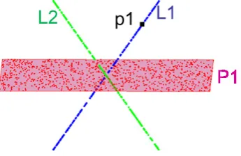
2.1 A toy example of subspace clustering. Three subspaces are contained in this example: two lines (L1, L2), and one plane (P1). . . 15
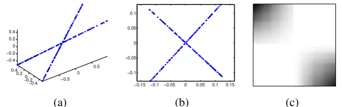
3.1 A toy example for subspace clustering: two lines L1 (with a point p) and L2 passing through the origin o form two independent linear subspaces. . . 36
3.2 Recovering a clean dictionary from noisy data with EDSC.(a) Data corrupted by Gaussian noise; (b) Optimal solution C∗ of (3.14); (c) Recovered clean dictionaryD. . . . 41
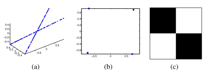
3.3 Recovering a clean dictionary in the presence of outliers with EDSC. (a) Data corrupted by noise and outliers; (b) Optimal solution C∗ of (3.16); (c) Recovered clean dictionaryD . . . 44
3.4 Sample images from the Hopkin155 dataset including indoor checker-board sequences, outdoor traffic sequences, non-rigid and articulated sequences. . . 45
3.5 Sample face images from the extended yale B face dataset: each row contains aligned face images of the same subject under different illu-mination conditions . . . 47
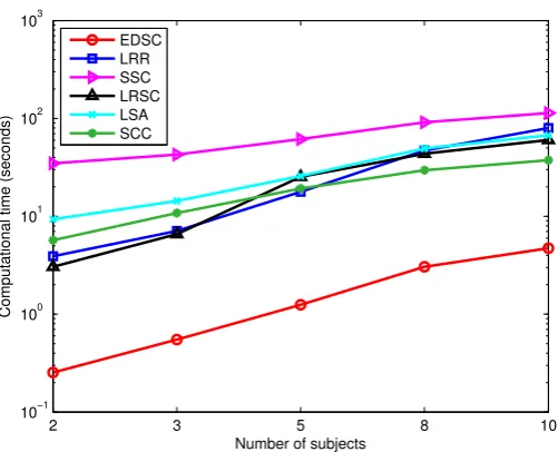
3.6 Average runtimes of the algorithms on Extended Yale B as a function of the number of subjects. . . 48
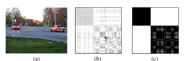
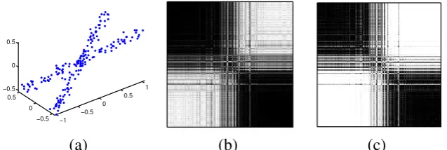
4.1 Subspace clustering example: (a) Two motions, each forming one subspace;(b)Shape Interaction Matrix of the trajectories in (a), which is sensitive to noise; (c) Affinity matrix obtained by our method: a much clearer block-diagonal structure. . . 50
4.2 SIM for clustering two lines in 3D: (a)Two lines (each forming one subspace) with an arbitrary angle; (b) New data representation with Vr. Note that the lines have become orthogonal; (c) SIM (absolute value) normalized by its maximum value; the darker the SIM image, the greater the value. . . 51 4.3 Clustering two lines in 3D: Row normalization (a)Two lines (each
forming one subspace) with an arbitrary angle;(b)New data represen-tation with row-normalizedVr. Note that the lines collapse four points on the unit circle, corresponding to orthogonal vectors;(c) New SIM (absolute value) without magnitude bias. . . 55 4.4 Clustering two lines with noise in 3D: (a)Two lines with Gaussian
noise; (b) New SIM after row normalization, with noise in the off-diagonal blocks;(c)Affinity matrix after elementwise powering. Note that the block-diagonal structure is much cleaner. . . 57 4.5 Comparison of SSC-R and RSIM-M on semi-dense data: While
SSC-R removes the trajectories with missing entries, and thus gets less dense results, our method can handle missing data robustly. Each image is a frame sampled from one of the video sequences. The points marked with the same color are clustered into the same group by the respective methods. Best viewed in color. . . 66 4.6 Typical behavior of SSC-O on semi-dense data:By treating missing
entries as outliers, SSC-O tends to cluster the trajectories with missing entries into same group. The points marked with the same color are clustered into the same group by SSC-O. Best viewed in color. . . 66 4.7 Failure cases of SSC-R and of RSIM-M: We conjecture that these
failures are due to tracking failures (e.g., very few trajectories), or to high dependence between motions. Best viewed in color. . . 67 4.8 Semi-dense motion segmentation results for sequences 1-4. Our method
(RSIM-M) uses all the available tracks (3026 on average) with an av-erage runtime of 5.22 seconds per sequence; SSC-O tends to group the trajectories with missing entries in the same cluster; SSC-R takes 150.48 seconds on average and only makes use of 2522 points on average after removing the incomplete trajectories. Best viewed in color. . . 68 4.9 Semi-dense motion segmentation results for sequences 5-10. Our method
4.10 Semi-dense motion segmentation results for sequences 11-16. Our method (RSIM-M) uses all the available tracks (3026 on average) with an average runtime of 5.22 seconds per sequence; SSC-O tends to group the trajectories with missing entries in the same cluster; SSC-R takes 150.48 seconds on average and only makes use of 2522 points on average after removing the incomplete trajectories. Best viewed in color. . . 70 4.11 Semi-dense motion segmentation results for sequences 17-18. Our
method (RSIM-M) uses all the available tracks (3026 on average) with an average runtime of 5.22 seconds per sequence; SSC-O tends to group the trajectories with missing entries in the same cluster; SSC-R takes 150.48 seconds on average and only makes use of 2522 points on average after removing the incomplete trajectories. Best viewed in color. . . 71
5.1 Motion segmentation with unknown correspondences: given a video sequence and feature points in each frame, our goal is to simultane-ously estimate motion clusters and feature matching. . . 74 5.2 (a) Convergence curves for the objective function value and the
pri-mal residuals. Blue curves: initialization (V1); red curves: initializa-tion (V2). (b)Accuracy of motion segmentation by adding different amounts of outliers and Gaussian noise. . . 84 5.3 Motion segmentation results of different algorithms for the cars2_07_g12
sequence. Points marked with the same color and marker (◦ or ×) are from the same motion: (a) SIFT + SSC; (b) RE + SSC (RE: ROML with embedded feature);(c)RS + SSC (RS: ROML with SIFT feature);(d)Our algorithm. Best viewed in color. . . 85 5.4 Motion segmentation results of the airport sequence: Points marked
with the same color and marker (◦ or ×) are from the same motion. Best viewed in color. . . 87
6.1 Performance of different trackers on the 1RT2TC checkerboard sequence: The red points denote the current positions of the feature points, and the green lines the motion since the previous frame. Best viewed zoomed-in on screen. . . 102 6.2 Performance of different trackers on the car1 sequence: The red
points denote the current positions of the feature points, and the green lines the motion since the previous frame. Best viewed in color. . . . 103 6.3 Tracking error as a function of the frame number: In these two
6.4 The MAN and MONK sequences of the MTPV dataset:The feature points are marked as red. Note that the number of points on the walking man and monk is much smaller than on the background. . . . 105 6.5 Performance of different trackers on the KITTI sequence: The
3.1 Clustering error (in %) on Hopkins155. . . 46
3.2 Clustering error (in %) on Extended Yale B. . . 48
4.1 Clustering error (in %) on Hopkins 155. . . 63
4.2 Ablation study on Hopkins 155. . . 63
4.3 Clustering error (in %) on Extended Yale B. . . 64
4.4 Clustering error (in %) on Hopkins 12 Real Motion Sequences with Incomplete Data. . . 65
5.1 Average motion segmentation and point correspondence accuracies (%) on the Hopkins155 27 non-checkerboard sequences. . . 86
5.2 Average motion segmentation and point correspondence accuracies (%) on the Hopkins155 checkerboard sequences with at most 200 trajectories. . . 86
6.1 Average number of tracking errors (ε = 10) on the Hopkins checker-board sequences with noise of different variances σ2. The lower, the better. . . 103
6.2 Average number of tracking errors (ε = 5) on the Hopkins Car-and-People sequences with noise of different variances σ2. The lower, the better. . . 103
6.3 Average number of tracking errors (ε = 5) on the MTPV sequences with noise of different variancesσ2. The lower, the better. . . 105
6.4 Average number of tracking errors (ε = 5) on the KITTI sequences with different noise variancesσ2. The lower, the better. . . 105
6.5 Average error rate (in%) of two-frame motion segmentation on the 22 Hopkins sequences with noise of different variances σ2. The lower, the better. . . 107
Introduction
Making a computer see as a human is the ultimate goal of computer vision research. Consider Figure 1.1(a) for the task ofobject-level segmentation. It takes no effort for us humans to tell which parts of the image belong to the same object. However, this remains a difficult task for a computer. Top-down learning based methods can get object-level segmentation, but the training phase requires numerous manually anno-tated images, which are normally expensive to acquire. Moreover, from the perspective of human vision, infants can learn to see without supplying them large amounts of carefully annotated images. In the same spirit, Geoffrey Hinton, a famous professor of machine learning, once said:
When we’re learning to see, nobody’s telling us what the right answers are – we just look. Every so often, your mother says "that’s a dog", but that’s very little information. You’d be lucky if you got a few bit of information – even one bit per second – that way. The brain’s visual system has1014
neural connections. And you only live for 109 seconds. So it’s no use learning one bit per second. You need more like105bits per second. And there’s only one place you can get that much information: from the input itself. – Geoffrey Hinton, 1996 (quoted in Murphy [2012]).
Modern bottom-up (unsupervised) segmentation methods rely on the information of the input itself, or more specifically the color and texture of the input, but only generate over-segmented small homogeneous regions, a.k.a. superpixels. For example, in Figure 1.1(b), with one of the state-of-the-art bottom-up segmentation methods, the car is segmented into multiple non-overlapping superpixels rather than a single object. We come into a dilemma here: on one hand, we do not want to rely on costly anno-tated training data for the task of object segmentation; on the other hand, unsupervised bottom-up methods such as superpixel segmentation methods, in most cases, cannot produce satisfactory object-level segmentation due to intrinsic ambiguities.
However, if we are given a video sequence and the objects in the sequence move for a period of time, these ambiguities can be easily resolved by leveraging constraints of temporal trajectories. Indeed, motion vectors are typically known to be more con-sistent than color and texture within an object region (Ochs et al. [2014]), especially
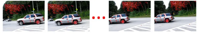
Figure 1.1: Left(a) Human can effortlessly tell which parts of the image belong to the same object. Middle (b) Superpixels generated by the method of Achanta et al. [2012]. Right(c) Motion vectors of a car sequence from Tron and Vidal [2007]: The red points denote the current positions of the feature points, and green lines the motion since the previous frame.
for rigid motions. For instance, in Figure 1.1(c), while color and texture are rather diverse within the car, the motion vectors of the feature points on the moving car have similar patterns.
Therefore, in this thesis, we focus on the study of motion segmentation, an impor-tant step towards object segmentation using unsupervised learning. In particular, the goal of motion segmentation is to group the pixels (or feature points) of a dynamic video sequence according to their motions. This is an important problem because its outcomes can be beneficial for many related areas in computer vision, such as scene understanding, video analysis, and multi-body structure from motion.
Generally, motion segmentation methods deal with feature tracks obtained by some feature tracking methods such as the Kanade-Lucas-Tomasi (KLT) feature tracker and optical flow. However, due to the drifting and occlusion problems in feature tracking, these feature tracks inevitably contain noise, outliers, or missing entries. One of our goals then is to design novel motion segmentation algorithms that are not only robust to these data corruptions, but also efficient in computations. We also consider the scenarios where the feature tracks are not available and aim to design algorithms that are able to solve for motion segmentation with unknown feature correspondences. In addition, we explore the possibility of improving current feature tracking methods by using additional scene constraints.
Before presenting the contributions of this thesis, we first review the related work on motion segmentation in literature.
1
.
1
Related Work
objects. By contrast, no special constraint on the camera motion is enforced for motion segmentation. Object tracking (Yilmaz et al. [2006]) is another related research area which tracks moving objects in the video with bounding boxes. In most cases, however, it requires manually specifying the objects to be tracked in the first frame. With a focus on motion segmentation in this thesis, we, therefore, do not discuss background subtraction and object tracking in more details.
Motion segmentation methods naturally fall into two categories: two-frame motion segmentation methods, and multi-frame motion segmentation methods.
1
.
1
.
1
Two-frame Motion Segmentation Methods
Most methods in this category rely on optical flow (Horn and Schunck [1981]; Brox et al. [2004]; Amiaz and Kiryati [2006]), which provides dense point correspondences between two consecutive frames. Early attempts at motion segmentation searched for discontinuities in the optical flow field (Thompson et al. [1985]; Black and Anandan [1990]), or piecewise affine partitions of the flow field (Adiv [1985]; Nagel et al. [1994]). These methods suffered from the fact that the optical flow at discontinuities is hard to recover due to occlusion.
Weber and Malik [1997] used the fact that each independently moving object corresponds to a unique epipolar constraint, or equivalently a unique fundamental matrix. The motion segmentation problem was formulated as minimizing a cost func-tional consisting of a data term that fits to the fundamental matrix and a discontinuity penalty term for spatial smoothness. The segmentation problem was solved via region-growing.
Klappstein et al. [2009] discussed the detection of moving objects in the context of driver assistance systems and road safety. Multiple constraints (i.e., epipolar con-straints, postive depth concon-straints, positive height concon-straints, and trifocal constraints) were used to compute a motion metric reflecting how likely a feature point to be moving.
Narayana et al. [2013] assumed that only translational motions were involved. Instead of using the complete flow vectors, they leveraged optical flow orientations for dense motion segmentation. However, in practice, the pure translational motion assumption is often too restrictive and does not hold as long as either the object or the camera motions are rotational.
Other methods (Brox et al. [2006]; Amiaz and Kiryati [2005]; Cremers and Soatto [2005a]; Mémin and Pérez [2002]; Brox and Weickert [2006]) tried to simultaneously solve for optical flow and segmentation with the variational method and the level-set based motion competition technique (Zhu and Yuille [1996]). The flow was estimated independently for each segmented region, and the region segmentation represented by level sets was driven by the fitting error of the optical flow.
segmenta-tion. However, they also suffer from the difficulties in estimating very accurate optical flow, especially in texture-less and occluded regions.
A few other two-frame motion segmentation methods rely on sparse feature corre-spondences between two views. For example, Li [2007] used a mixture-of-fundamental-matrices model to describe the multi-body motions from two views, and with a ran-dom sampling scheme (Fischler and Bolles [1981]), solved the problem via a linear program relaxation. In essence, this method tried to solve a chicken-and-egg problem, and alternated between solving for multiple fundamental matrices and updating the motion assignment in an Expectation Maximization (EM) manner, which is sensitive to initialization.
Vidal et al. [2006] derived a multi-body epipolar constraint and its associated multi-body fundamental matrix from noise-free sparse point correspondences of two perspective views. The epipolar lines and epipoles were then computed using an algebraic geometric approach. Given the epipolar lines and the associated multiple fundamental matrices, the clustering was obtained by assigning each point to its near-est fundamental matrix based on the Sampson distance. As pointed out by the authors, this approach was mostly designed for noise-free correspondences and is thus sensitive to noise and outliers.
On a frame-to-frame level, Dragon et al. [2012] employed a motion-split-and-merge approach that consists of splitting the tracklets with J-Linkage (Toldo and Fusiello [2008]) until the segments are consistent and merging with neighbouring segments until the algorithm converges. This method was improved for real time performance by Dragon et al. [2013]. Elqursh and Elgammal [2013] formulated motion segmen-tation as a manifold separation problem and presented an online method using label propagation on a dynamically changing graph.
All in all, two-frame methods suffer from the fact that motions between consecu-tive frames are relaconsecu-tively small and thus motion segmentation from two frames is often ambiguous.
1
.
1
.
2
Multi-frame Motion Segmentation Methods
Multi-frame motion segmentation methods are generally more robust than two-frame methods. Most of the recent works on motion segmentation belong to this class. Typically, point trajectories over frames are assumed to be given a priori from the KLT tracker or more recent feature tracking methods (e.g., Sundaram et al. [2010]). See Figure 1.2 for an example. Then the affinities between trajectories are constructed in a way that those from the same motion have high affinity and those from different motions have low affinity (or ideally zero affinity). With the affinity matrix, the final motion segmentation is obtained by the normalized cuts (Shi and Malik [2000]) or spectral clustering (Ng et al. [2002]).
pos-Figure 1.2: Multi-frame motion segmentation with feature tracks over frames.
sibly different length. Brox and Malik [2010] and Ochs et al. [2014] defined affinities with pairwise distances between trajectories, and used a spatially regularized spectral clustering for segmentation. However, the pairwise distance only accounts for the translational model, and thus cannot handle other motion models such as rotation and scaling. A follow-up work by Ochs and Brox [2012] addressed this limitation by using higher order tuples of trajectories to form hypergraphs. To apply spectral clustering, the hypergraph was flattened into an ordinary graph via a nonlinear projection, i.e., a regularized maximum operator. Unfortunately, although sampling techniques were applied, the high order motion models still resulted in high computational complexity.
Other works leveraged explicit camera models, e.g., the perspective camera model or affine camera model, to derive trajectory affinities. Under the perspective camera model, Jung et al. [2014] iteratively computed fundamental matrices and motion la-bels. Evidence of segmentation was then accumulated across frames via randomized voting based on the Sampson distance between the point and the epipolar line. Li et al. [2013] derived a subspace method from the two-view epipolar constraint, and formu-lated the motion segmentation from multiple frames as a mixed norm optimization problem. A model selection method was also proposed based on an over-segment-and-merge procedure.
The affine camera model is commonly used as an approximation of the perspective camera model where depth variation of the scene is negligible compared to the overall scene depth. It has been proven that, under the affine camera model, trajectories from the same motion lie in a linear subspace with dimension up to four and trajectories from different motions correspond to different subspaces (Yan and Pollefeys [2006]). Under the affine camera model assumption, the motion segmentation problem can be solved as a subspace clustering problem. Thanks to the useful property of this subspace formulation, a large amount of work follows this direction.
[image:25.595.110.525.113.186.2]Factorization Based Algorithms
Factorization based algorithms (Boult and Brown [1991]; Costeira and Kanade [1998]; Gear [1998]), initially introduced for motion segmentation, achieve segmentation by a low-rank factorization of the data matrixX whose columns represent the data points. To group data into corresponding subspaces, Costeira and Kanade [1998] relied on the Shape Interaction Matrix (SIM), which was defined asQ = VVT ∈ RN×N, withV the matrix consisting of right singular vectors ofXand N the number of trajectories. The matrixQhas the property thatQij =0if pointsiandjlie in different subspaces. Segmentation was achieved by simply block-diagonalizingQ, or by applying spectral clustering.
Kanatani [2001] later analysed motion segmentation as a subspace segmentation problem, and showed that under the condition that the subspaces are linearly inde-pendent, the SIM is block-diagonal up to a permutation. Many other methods (Gear [1998]; Ichimura [1999]; Kanatani [2002]; Wu et al. [2001]; Zelnik-Manor and Irani [2003]) were proposed to improve the robustness of the SIM method. Unfortunately, they are sensitive to noise and outliers, and require a reliable estimation of the intrinsic dimension of the data matrix.
Inspired by the theory of non-negative matrix factorization (Lee and Seung [1999]), Cheriyadat and Radke [2009] decomposed the velocity profiles of point trajectories into different motion components and corresponding non-negative weights, and then segmented the motions using spectral clustering on the derived weights. Similarly, Mo and Draper [2012] modeled dense point trajectories with a semi-non-negative matrix factorization method to get semantically meaningful motion components.
Algebraic Methods
Expectation Maximization Based Approaches
Expectation Maximization (EM) based approaches estimate subspace models and as-signments iteratively. For example, K-planes (Bradley and Mangasarian [2000]) and K-subspaces (Tseng [2000]) algorithms extended the K-means method (MacQueen et al. [1967]; Duda et al. [2012]) (which is an EM based method) to clustering data sampled from multiple planes or subspaces. The two algorithms iterated over the following two steps until converge: 1) given an initial cluster assignment, fit a sub-space/plane for each cluster with PCA; 2) with the PCA basis for each subsub-space/plane, assign each data point to its nearest subspace/plane. These methods suffer from two drawbacks: first, the problems they solved are nonconvex, so the solution depends on initialization; second, the PCA subspace/plane fitting step is sensitive to outliers.
A few other methods (e.g., Tipping and Bishop [1999]; Ma and Derksen [2007]) addressed the subspace clustering problem within a probabilistic framework. In sta-tistical learning, mixed data are often modeled as samples drawn from mixtures of Gaussian distributions. In this context, subspace clustering becomes a model fitting problem. A major drawback of this approach, however, is that it often results in non-convex optimization problems. One therefore has to resort to an EM method, whose solution strongly depends on initialization.
High-order Model Based Methods
High-order model based methods try to fit a pre-defined model with multiple trajec-tories (or points). In particular, Local Subspace Affinity (LSA) (Yan and Pollefeys [2006]) fitted a linear subspace at each trajectory with local adjacent trajectory sam-pling, and then derived the affinity matrix based on the principal subspace angles between these estimated subspaces. Alternatively, LSA can also be interpreted as using the projection distance of points on the Grassmann manifold because a subspace can be viewed as a point on the corresponding Grassmann manifold. However, this local subspace fitting can be unreliable due to various data corruptions, especially for points lying close to subspace intersections.
Chen and Lerman [2009] proposed a Spectral Curvature Clustering (SCC) method using the polar curvature of d+2 distinct points (withd the subspace dimension) to form the affinity tensor. To make it computationally tractable, an iterative sampling procedure was suggested to reduce the affinity tensor to an affinity matrix.
Jain and Govindu [2013] presented Sparse Grassmann Clustering (SGC) that uti-lized the residual error of fitting a high dimensional model (with at leastd+2points) to construct affinities. The efficiency of the algorithm was gained by updating the eigenspace of the affinity matrix via an efficient Grassmannian gradient descent method and iterative sampling.
Similarly, Purkait et al. [2014] also used model fitting residuals to build affinities, but with more points (much more than d+2), thus leading to large hyperedges of hypergraphs. A novel guided sampling strategy for large hyperedges was proposed based on the concept of random cluster models to reduce the sampling costs.
High-order model based methods can be applied to solve general model fitting and clustering problems. However, in many cases, explicit models are required to knowa priori, and the computational complexity still remains to be a limiting factor of this type of methods.
Self-expressiveness Based Algorithms
Recently, self-expressiveness based algorithms (Elhamifar and Vidal [2009]; Liu et al. [2010]; Favaro et al. [2011]; Elhamifar and Vidal [2010]; Liu et al. [2013]; Elhamifar and Vidal [2013]) have received much attention in the research community. The data drawn from multiple subspaces are deemed self-expressive in the sense that a data point in a subspace can be represented as a linear combination of the other points in the same subspace. The affinity matrix can then be constructed by the linear combination coefficient matrix. Relating back to the high-order model based methods, by self-expressiveness, a point (or trajectory) is in fact connected to all the other points simultaneously, which can be thought of as virtually applying the highest-possible-order model. This, to some extent, explains the recent popularity and success of this kind of methods.
The most popular approaches in this category were inspired by the theory of com-pressive sensing. In particular, Sparse Subspace Clustering (SSC) (Elhamifar and Vidal [2009]) employed the data matrix as a dictionary to reconstruct the data itself. It then utilized the coefficients recovered by an `1-norm minimization problem to construct an affinity matrix whose non-zero entries correspond to points in the same subspace. Similarly, Low Rank Representation (LRR) (Liu et al. [2010]) exploited the self-expressiveness of the data, but, instead of sparsity, assumed that the coefficient matrix has low rank.
clustering method. There are also several non-linear extensions of SSC, such as (Patel et al. [2013]), (Patel and Vidal [2014]) and (Yin et al. [2016]).
While both SSC and LRR solved the problem formulations in an iterative manner, a closed-form solution was introduced in Low-Rank Subspace Clustering (LRSC) (Favaro et al. [2011]), which, for noisy data, involved performing a series of singular value thresholding operations. To derive this closed-form solution, LRSC relied on recovering a clean dictionary instead of directly making use of the noisy data.
Other types of regularization on the self-expressiveness include using the quadratic programming (Wang et al. [2011b]), the latent low rank representation (Liu and Yan [2011]), the least square regression (Lu et al. [2012]), the trace lasso (Lu et al. [2013]), the half-quadratic minimization (Zhang et al. [2013]), the block-diagonal prior (Feng et al. [2014]), the smooth representation (Hu et al. [2014]), a structured norm (Li and Vidal [2015]), the Gaussian mixture regression (Li et al. [2015]) and the elastic net (You et al. [2016]).
The nice property of this class of methods is that in most cases, the resulting prob-lem formulations are convex, so global optimal solutions can be achieved. However, to apply self-expressiveness for motion segmentation, these methods require the point trajectories to be of the same length and thus cannot naturally handle the case of missing data, whose presence is inevitable in real-world scenarios.
1
.
2
Contributions
This thesis focuses onmulti-framemotion segmentation with subspace constraints and aims to handle various types of data corruption in a robust and efficient manner. The contributions are three-fold: first, we present novel subspace clustering algorithms that can be directly applied to motion segmentation; second, we tackle the motion segmentation problem under unknown feature correspondences and give a solution that simultaneously performs motion segmentation and feature matching; third, we develop a segmentation-free multi-body feature tracking method using the subspace constraint derived from epipolar geometry.
Novel Subspace Clustering Algorithms
Two novel subspace clustering methods are presented in this thesis, namely Efficient Dense Subspace Clustering (EDSC), and the Robust Shape Interaction Matrix (RSIM) method.
the subspace clustering problem efficiently. More specifically, the solution can be obtained in closed-form for outlier-free observations, and by performing a series of linear operations in the presence of outliers. Furthermore, we show that our Frobenius norm formulation shares the same solution as the popular nuclear norm minimization approach when the data is free of any noise.
In RSIM, we revisit the Shape Interaction Matrix (SIM) method, one of the earliest approaches for motion segmentation (or subspace clustering), and reveal its connec-tions to several recent subspace clustering methods. We derive a simple, yet effective algorithm to robustify the SIM method and make it applicable to real-world scenarios where the data is corrupted by noise. We validate the proposed method by intuitive examples and justify it with the matrix perturbation theory. Moreover, we show that RSIM can be extended to handle missing data with a Grassmannian gradient descent method.
Both the above-mentioned subspace clustering algorithms (i.e., EDSC and RSIM) can be applied to motion segmentation with robustness to data noise, outliers, and missing data, which is evidenced by our experiments on standard motion segmentation datasets, such as Hopkins 155 (Tron and Vidal [2007]).
Motion Segmentation with Unknown Correspondences
Motion segmentation can be addressed as a subspace clustering problem, assuming that the trajectories of interest points are known. However, establishing point spondences is in itself a challenging task. Most existing approaches tackle the corre-spondence estimation and motion segmentation problems separately. In this part, we develop an approach to performing motion segmentation without any prior knowledge of point correspondences. We formulate this problem in terms of Partial Permutation Matrices (PPMs) and aim to match feature descriptors while simultaneously encourag-ing point trajectories to satisfy subspace constraints. This lets us handle outliers in both point locations and feature appearance. The resulting optimization problem is solved via the Alternating Direction Method of Multipliers (ADMM), where each subproblem has an efficient solution. In particular, we show that most of the subproblems can be solved in closed-form, and one binary assignment subproblem can be solved by the Hungarian algorithm.
Robust Multi-body Feature Tracker
This approach, however, requires knowing the number of motions, as well as assigning points to motion groups, which is typically sensitive to motion estimates. By contrast, we introduce a segmentation-free solution to multi-body feature tracking that bypasses the motion assignment step and reduces to solving a series of subproblems with closed-form solutions.
Summary of Contributions
In summary, in this thesis, we exploit the powerful subspace constraints and present motion segmentation methods that are robust to various types of data corruptions in the cases of known or unknown feature correspondences. In addition, we also propose a robust feature tracker for dynamic scenes, which can be applied to get reliable trajectories for motion segmentation.
1
.
3
Thesis Structure
Preliminaries
2
.
1
Basic Notations
Throughout this thesis, we denote matrices by bold upper case letters, vectors by bold lower case letters, and scalars by non-bold letters. Upper case non-bold letters are also used to denote a space, subspace or field. R, RN, andRD×N are respectively the set of real numbers, the set of real N-dimensional vectors, and the set of real D-by-N matrices.
We organize the point trajectories as the columns of the data matrixX ∈ RD×N, and the ith column (or trajectory) of X is represented by xi. The transpose of X is denoted by XT. The vectorization ofX, denoted byvec(X), is obtained by stacking the columns ofX, i.e.,vec(X) = [x1T| · · · |xTN]T. The identity matrix is denoted byI, and the all-one column vector is denoted by1. The full Singular Value Decomposition (SVD) of X is expressed as X = UΣVT with U ∈ RD×p (p = min(D,N)) and V ∈ Rp×N being orthonormal matrices, andΣ ∈ Rp×p the diagonal matrix whose diagonal elements are the singular values of X. If X is low-rank with the rank r <
min(D,N), its compact SVD can be written asX=UrΣrVTr, whereUr contains the firstrcolumns ofU, Vr the firstrcolumns of V, andΣr the firstrsingular values on its diagonal.
Vector or matrix norms are commonly used. For a vector x, its `0 norm kxk0 is defined as the number of non-zero elements ofx; its`pnormkxkp (forp=1, 2,· · ·) is defined askxkp = ∑i|xi|p
1/p
, e.g.kxk1 =∑i|xi|; its`∞norm is defined as the maximal element of|x|, i.e. kxk∞ =maxi|xi|. By default,kxk denotes the`2norm ofx. A matrix norm is a natural extension of a vector norm. Specifically, for element-wise matrix norms, kXk1 = ∑i,j|xij|, the Frobenius norm kXkF =
q
∑i,jx2ij = p
trace(XTX), the `
p norm kXkp = ∑i,j|xij|p 1/p
, and the `2,1 norm kXk2,1 =
∑jkxjk = ∑j q
∑ix2ij. Another widely used norm is the nuclear norm (also known as trace norm), which is defined askXk∗ =∑iσi withσitheith singular value ofX.
The pseudoinverse (also known as Moore-Penrose pseudoinverse) of Xis denoted byX†. It has the following properties: 1)XX†X=X; 2)X†XX† =X†; 3)(XX†)T =
XX†; 4) (X†X)T = X†X. If the columns of X are linearly independent, then XTX is invertible. In this case, the pseudoinverse of X can be explicitly written as X† = (XTX)−1XT. Similarly, if the rows ofXare linearly independent,X† =XT(XXT)−1. A simple way to compute the pseudoinverse is by the SVD. Given the SVD of X as X = UΣVT, X† = VΣ−1UT. The pseudoinverse can be used to solve for a least squares solution to a system of linear equations. For example, given a systemAy =b with y the unknown, the best solution in the sense of the least squares error can be computed asy∗ =A†b.
The Kronecker product is denoted by ⊗. For two matricesA ∈ Rm×n and B ∈
Rp×q, their Kronecker product is defined as
A⊗B=
a11B · · · a1nB ..
. . .. ... am1B · · · amnB
∈ R
mp×nq . (2.1)
The Kronecker product is useful to solve some linear systems in matrix form. For example, consider the equation AYB = C, where A, B and C are given, and Y is unknown. We can vectorize both sizes of the equation and get the following equation
vec(AYB) = (BT⊗A)vec(Y) =vec(C). (2.2)
2
.
2
Basic Concepts
2
.
2
.
1
Subspace
2.2.1.1 Linear Subspace and Affine Subspace
In linear algebra, the concept of subspace1is directly related to that of a vector space. A vector space is a mathematical structure that is closed under addition and scalar multiplication. A common example of a vector space is the Euclidian space. A subspace, which in itself is a vector space, is a subset of some higher-dimensional space. More formally, given a vector space V over a field F, it is often possible to form another vector space by taking a subsetWofVusing the vector space operations (i.e., additionandscalar multiplication) of V. To show whether a subset of a vector space is a subspace, we have the following theorem:
Theorem 2.1 (Leon [2010]) LetV be a vector space over the field F, and letW be a nonempty subset ofV. ThenW is a subspace ofV if and only ifW satisfies the following three conditions
1. The zero vector0is inW.
Figure 2.1: A toy example of subspace clustering. Three subspaces are contained in this example: two lines (L1, L2), and one plane (P1).
3. If u is an element of W and c is a scalar from F, then the product cu is an element ofW.
Condition 1 is one of the axioms that define the vector space and should be the first condition to verify when defining the subspace. Condition 2 states that W is closed under addition, which means that the sum of two elements ofW is always an element ofW. Condition 3 says thatWis closed under scalar multiplication. That is, whenever an element ofWis multiplied by a scalar, the result is still an element ofW. Therefore, if we use the operations from V and the elements ofW to do arithmetic, the results will always be inW. Another way to characterize subspaces is that they are also closed under linear combinations.
For example, in Figure 2.1, the lines L1andL2, and the planeP1(which intersect at the origin) are three subspaces of the 3D Euclidean space: the zero vector (the origin) is included in L1, L2 and P1; and it can be easily verified that they are all closed under the operations of addition and scalar multiplication.
Anaffine subspace, also known as aflat, is similar to a linear subspace except that it does not need to pass through the origin. For example, any line in the 2D Euclidean space forms an affine subspace or flat, but only those going through the origin are linear subspaces.
2.2.1.2 Null Space, Row Space and Column Space
Consider a matrixX ∈ RD×N. Let N(X)be the set of the solutions of the homoge-neous equationXc =0. We have
N(X) = {c∈ RN|Xc =0}. (2.3)
and henceαc∈ N(X). Ifc1,c2 ∈ N(X), then
X(c1+c2) = Xc1+Xc2=0,
which indicates thatc1+c2 ∈ N(X). It then follows thatN(X)is a subspace ofRN, and we callN(X)thenull spaceofX.
If we consider each row ofXas a vector inR1×N, the subspace ofR1×N spanned by the row vectors of Xis called the row space ofX. Similarly, the subspace ofRD spanned by the column vectors of X is called the column space of X. Note that the dimension of the row space ofXis equal to the dimension of the column space ofX.
A subspace can be represented by a set of orthogonal basis with the number of basis equal to the dimension of the subspace. So given a rank-rmatrixX(wherer ≤
min(D,N)) and its full SVDX=UΣVT, the column space ofXcan be represented byUr (i.e., the firstrcolumns ofU), the row space ofXbyVr(i.e., the firstrcolumns ofV), and the null space ofXbyVr+1:end(i.e., the last N−rcolumns ofV).
2.2.1.3 Subspace Clustering
With the definition of a subspace, the problem of subspace clustering is somewhat self-explanatory. Formally, suppose that we are given a set ofNdata pointsx1,x2,· · · ,xN
∈ RD and that these data points are drawn from a union of K subspaces{S
i}Ki=1 of unknown dimensions. Then the goal of subspace clustering is to cluster the data points into their respective subspaces, or in plain words, to find which data point lies on which subspace. For example in Figure 2.1, we aim to cluster the points according to three subspaces L1, L2 and P1, and different subspaces are plotted with different colors. In practice, the data points are often contaminated by noise and/or outliers, and some entries can even be unobserved. Thus, a practical subspace clustering method should be able to handle these data corruptions.
Affine subspaces are also within the scope of discussion of subspace clustering. In fact, an affine subspace can be thought of as lying on a higher dimensional linear subspace. For example, a line not going through the origin, which is an affine subspace, also lies on the plane going through the line and origin, which is a linear subspace. In literature (Chen and Lerman [2009]; Zhang et al. [2010]), subspace clustering is also calledHybrid Linear Modeling(HLM) when the data can be well approximated by a mixture of affine subspaces, or equivalently flats.
2
.
2
.
2
Grassmann Manifold
A point S on the Grassmann manifold G(N,r) is an r-dimensional linear subspace, which can be specified by an arbitrary orthogonal matrix U ∈ RN×r whose columns span the subspace S. Note that the matrix representation for a point on G(N,r) is not unique. For example, if the orthogonal matrix U ∈ RN×r represents a point on the Grassmannian G(N,r), thenUQ (with Qan arbitrary orthogonal r-by-r matrix) denotes the same point onG(N,r).
On a Grassmann manifold, the shortest distance between two points is along the geodesic, which is the curve of shortest length between two points on a manifold. To develop optimization algorithms (such as gradient methods), it is essential to compute a gradient step along the geodesic on the Grassmann manifold. To this end, we have the following theorem:
Theorem 2.2(Edelman et al. [1998])Given an optimization problem
min
Y∈G(N,r) f(Y) , (2.4)
and an initialization Y(0) = Y and its regular gradient d fdY = H, an update of Y along the geodesic with a step sizeηis given by
Y(η) = YV U
cos(Ση)
sin(Ση)
VT , (2.5)
whereUΣVT is the SVD ofH.
The proof of Theorem 2.2 is provided in (Edelman et al. [1998]). Various gradient methods (such as conjugate gradient and Newton’s method) on the Grassmann mani-fold can be developed with this theorem. Interested readers may refer to Edelman et al. [1998] for more details.
2
.
3
Subspace Formulation for Motion
Segmenta-tion
2
.
3
.
1
Affine Camera Model
According to Hartley and Zisserman [2004], anaffine camerais one that has a camera matrixP in which the last row is of the form(0, 0, 0, 1); it is called an affine camera because points at infinity are mapped to points at infinity. The affine camera model is widely used as an approximation to the perspective camera model when the variation of the depth of the scene is much smaller than the distance of the points to the image plane (Ma et al. [2012]).
orthographic, weak perspective and paraperspective models, a 3D point[X,Y,Z]T in space is projected to a 2D point[x,y]T on the image plane as
x y 1
=K
1 0 0 0 0 1 0 0 0 0 0 1
R t 0T 1
X Y Z 1 , (2.6)
where K ∈ R3×3 is the matrix of intrinsic camera parameters, and R ∈ R3×3 and t ∈ R3are camera rotation and translation, respectively. So we can write the camera matrix of an affine camera as
P =K
1 0 0 0 0 1 0 0 0 0 0 1
R t 0T 1
. (2.7)
It is easy to see thatPhas the form
P=
m11 m12 m13 t1 m21 m22 m23 t2
0 0 0 1
, (2.8)
where we can define the affine motion matrixM ∈R2×4as
M=
m11 m12 m13 t1 m21 m22 m23 t2
. (2.9)
Thus, projection under an affine camera model can be expressed as
x y =M X Y Z 1 . (2.10)
2
.
3
.
2
Factorization
If we assume that a moving affine camera observes the 3D point [X,Y,Z]T over F frames2, then we have F camera motion matrices M1,· · · ,MF. Stacking the image
points[xi,yi]T (i =1,· · · ,F) into a trajectory vector leads to x1 y1 .. . xF yF = M1 .. . MF X Y Z 1 , (2.11)
where we can define the total camera motion matrixWas
W= M1 .. . MF ∈ R
2F×4. (2.12)
Now, we considerNimage points in theithframe projected fromNpoints[Xj,Yj,Zj]T of a rigid body over an affine cameraMi
xi1 xi2 · · · xiN yi1 yi2 · · · yiN
=Mi
X1 · · · XN Y1 · · · YN Z1 · · · ZN
1 · · · 1
, (2.13)
where we define the shape matrixSas
S=
X1 · · · XN Y1 · · · YN Z1 · · · ZN
1 · · · 1
∈ R4×N . (2.14)
If we stack all the Nfeature points inFframes together, we have
x11 x12 · · · x1N y11 y12 · · · y1N
..
. ... . .. ... xF1 xF2 · · · xFN yF1 yF2 · · · yFN
| {z }
X∈R2F×N
= M1 .. . MF
| {z } W∈R2F×4
X1 · · · XN Y1 · · · YN Z1 · · · ZN
1 · · · 1
| {z }
S∈R4×N
, (2.15)
Thus, the trajectory matrixXcan be factorized into a bilinear form as
X =WS. (2.16)
Note that the factorization ofXis unique since for any invertible matrixQ ∈R4×4, X = WQ
Q−1S
. For Eq. (2.16), if we take the four columns of W as the four basis of a linear subspace with intrinsic dimension 4 and ambient dimension2F, then the elements of S are the coefficients, and the columns of X become points in this subspace. So, under an affine camera model, one motion corresponds to one linear subspace with dimension at most four. Alternatively, since the last row ofSis1T, the trajectories on the image planes of a rigid motion lie in an affine subspace ofR2F with dimension at most three (Elhamifar and Vidal [2009]).
Naturally, for Krigid motions, we can still factorize the data matrix as
X =
X1 · · · XK
=
W1S1 · · · WKSK
=
W1 · · · WK
S1 . ..
SK
,
(2.17)
where Wi is the motion matrix for theith motion, and Si is the shape matrix for the ith rigid body. Note that, in practice, the trajectories are not sorted according to their motions, so this factorization works up to certain permutations of the columns ofX.
We can see that the trajectories ofK motions lie in a union of linear subspaces of dimension up to 4K. Thus under the affine camera model, the motion segmentation problem can be addressed as a subspace clustering problem.
2
.
3
.
3
Self-expressiveness
Mathematically, the property of self-expressiveness can be summarized as one single equation
X =XC, (2.18)
where X is the data matrix with each column being one data point, and C is the coefficient matrix.
To employ this idea to construct an affinity matrix, one has to ensure that the coef-ficient matrixChas nonzero entries only for the points in the same subspaces. In other words,Cij =0if points iand jbelong to different subspaces, andCij 6=0otherwise. This can be achieved by minimizing certain norms ofC. In particular, inspired by the compressive sensing theory, SSC (Elhamifar and Vidal [2013]) minimizes the`1norm ofCto get sparse representation of the data:
min
C kCk1 (2.19)
s.t. X=XC, diag(C) =0 ,
where the diagonal constraint is enforced to avoid the trivial solution (i.e., the identity matrix).
For affine subspaces, an additional constraint onCcan be incorporated to enforce the sum of each column ofCto be 1, i.e.,
min
C kCk1 (2.20)
s.t. X=XC,
1TC=1T, diag(C) =0 .
Alternatively, one could also add an extra all-one row toXso that the affine constraint is implicitly enforced.
When the data contain noise and some sparse outliers, the equality constraintX= XC does not hold. This case can be handled by adding extra regularization terms in the cost function (Elhamifar and Vidal [2013]),
min
C kCk1+
λ1
2 kE1k
2
F+λ2kE2k1 (2.21)
s.t. X=XC+E1+E2, 1TC =1T,
diag(C) = 0,
are parameters.
To get low-rank representation, LRR (Liu et al. [2013]) minimizes the nuclear norm ofC:
min
C kCk∗ s.t. X =XC. (2.22)
A slightly different way to handle data corruptions is by modeling them with a structured norm on the noise term (Liu et al. [2013]):
min
C,EkCk∗+λkEk2,1 (2.23)
s.t. X=XC+E,
whereEmodels the data corruptions. Since each column ofXrepresents a data point, the `2,1 norm regularization on the noise term E then assumes that only a few data points (or columns ofX) are grossly corrupted.
2
.
3
.
4
Spectral Clustering
Most motion segmentation methods consist of first building an affinity matrix in some way (Yan and Pollefeys [2006]; Chen and Lerman [2009]; Elhamifar and Vidal [2009]; Liu et al. [2010]) and then applying spectral clustering with the affinity matrix to get the final segmentation results. So spectral clustering is an important tool for the motion segmentation task. Here, we follow von Luxburg [2007] to give a brief introduction to spectral clustering.
The spectral clustering algorithms rely on the construction of a Laplacian matrix. In literature, there are two types of Laplacian matrices, i.e., unnormalized Laplacian and normalized Laplacian.
2.3.4.1 Unnormalized Spectral Clustering
Suppose we have a nonnegative symmetric affinity matrix A ∈ RN×N where a ij = aji ≥0. Equivalently,Aalso describes an undirected, weighted graph Gwith weight matrixA. Theunnormalized Laplacian matrixis defined as
Lun =D−A, (2.24)
whereDis the diagonal degree matrix defined as
D=
∑ja1j · · · 0 ..
. . .. ...
0 · · · ∑jaNj
or in other words, theith elementdi on the diagonal ofDis the sum of theith row of A. Lunispositive semi-definitebecause, for every vectorf∈ RN, we have
fTLunf =fTDf−fTAf (2.26)
=
N
∑
i=1 difi2−
N
∑
i,j=1
fifjwij (2.27)
= 1
2
N
∑
i=1
difi2−2 N
∑
i,j=1
fifjwij+ N
∑
j=1 djfj2
(2.28) = 1 2 N
∑
i,j=1
wijfi2−2 N
∑
i,j=1
fifjwij+ N
∑
j,i=1 wjifj2
(2.29) = 1 2 N
∑
i,j=1
wijfi2−2 N
∑
i,j=1
fifjwij+ N
∑
i,j=1 wijfj2
(2.30) = 1 2 N
∑
i,j=1
wij(fi− fj)2 ≥0 . (2.31)
By observation, it is obvious that the smallest eigenvalue of Lun is 0 and the corre-sponding eigenvector is the constant one vector1.
One of the important properties of the unnormalized Laplacian is summarized in the following proposition.
Proposition 2.1LetGbe an undirected graph with non-negative weightsA. Then the multiplicity kof the eigenvalue 0of Lun equals the number of connected compo-nents A1,· · · ,Ak in the graph. The eigenspace of eigenvalue 0 is spanned by the indicator vectors1A1,· · · ,1Ak of those components.
The proof is given in (von Luxburg [2007]). This proposition says that the num-ber of clusters is equal to the multiplicity of the eigenvalue 0 of the unnormalized LaplacianLunand the clustering is indicated by the eigenvectors of eigenvalue0.
With this proposition, the unnormalized spectral clustering algorithm can be writ-ten as
Algorithm 2.1Unnormalized spectral clustering
Input: Affinity matrixA∈ RN×N, number of clustersk 1. Compute the unnormalized LaplacianLun as in (2.24).
2. Compute the smallest k eigenvectorsu1,· · · ,uk ofLun, and form U ∈ RN×k withu1,· · · ,ukas columns. Each row ofUis denoted byyi ∈ Rk,i =1,· · · ,N. 3. Cluster the points {yi}i=1,···,N with thek-means algorithm and get the cluster label vectors∈ {1,· · · ,k}N.
2.3.4.2 Normalized Spectral Clustering
In literature, there are two ways to normalize the Laplacian matrix, i.e.,
Lsym =D−1/2LunD−1/2 =I−D−1/2LunW−1/2 (2.32) Lrw=D−1Lun =I−D−1W, (2.33)
whereLsymis a symmetric matrix, andLrwis closely related to a random walk. Similarly to the unnormalized Laplacian Lun, the normalized Laplacians Lsym and Lrw are both positive semi-definite and have 0 as the smallest eigenvalue. The corresponding eigenvector of Lrw is the constant one vector 1, and that of Lsym is D−1/21.
As in the unnormalized Laplacian, the multiplicity of the eigenvalue 0 of the normalized LaplaciansLsymandLrwis also related to the number of clusters.
Proposition 2.2LetGbe an undirected graph with non-negative weightsA. Then the multiplicitykof the eigenvalue0of bothLrwandLsymequals the number of con-nected componentsA1,· · · ,Akin the graph. ForLrw, the eigenspace of eigenvalue0 is spanned by the indicator vectors1A1,· · · ,1Ak of those components. ForLsym, the
eigenspace of eigenvalue0is spanned by the indicator vectorsD−1/21A1,· · · ,D−1/2 1Ak.
This leads to two versions of the normalized spectral clustering algorithm.
Algorithm 2.2Normalized spectral clustering according to Shi and Malik [2000] Input: Affinity matrixA∈ RN×N, number of clustersk
1. Compute the unnormalized LaplacianLunas in (2.24).
2. Compute the smallest k generalized eigenvectors u1,· · · ,uk of Lun of the generalize eigenproblem Lunu = λDu, and form U ∈ RN×k with u1,· · · ,uk as columns. Each row ofUis denoted byyi ∈ Rk,i =1,· · · ,N.
3. Cluster the points {yi}i=1,···,N with thek-means algorithm and get the cluster label vectors∈ {1,· · · ,k}N.
Output: The cluster labels
Note that in algorithm 2.2 the generalized eigenvectors of Lun are equivalent to the eigenvectors of Lrw. This algorithm can be interpreted from a perspective of normalized graph cuts, so it is also called the normalized cuts algorithm (Shi and Malik [2000]).
Algorithm 2.3Normalized spectral clustering according to Ng et al. [2002] Input: Affinity matrixA∈ RN×N, number of clustersk
1. Compute the normalized LaplacianLsym as in (2.32).
2. Compute the smallestkeigenvectorsu1,· · · ,uk ofLsym, and form U ∈ RN×k withu1,· · · ,ukas columns. Each row ofUis denoted byyi ∈ Rk,i =1,· · · ,N. 3. Normalizeyito getti =yi/kyikfori =1,· · · ,N.
4. Cluster the points {ti}i=1,···,N with the k-means algorithm and get the cluster label vectors∈ {1,· · · ,k}N.
Output: The cluster labels
The algorithms 2.1, 2.2 and 2.3 all look rather similar, except that they use dif-ferent Laplacian matrices. We can see that the main trick of all three algorithms is to change the representation of the data points xi to points yi ∈ Rk which are the eigenvectors of the Laplacian matrices, which enhances the cluster-properties in the new representation. With that, we simply apply the k-means clustering algorithm to detect the clusters in this new data representation. It has bee shown in this literature that the normalized spectral clustering algorithms generally perform better than the unnormalized one (von Luxburg [2007]). So in the remainder of this thesis, when mentioning spectral clustering, we always refer to normalized spectral clustering.
2
.
4
Optimization Methods
2
.
4
.
1
Alternating Direction Method of Multipliers
We follow Boyd et al. [2011] to introduce the Alternating Direction Method of Multi-pliers (ADMM), a widely used method for solving convex optimization problems with a large number of variables. ADMM works by decomposing a large optimization prob-lem into a set of smaller subprobprob-lems which are easier to handle. Before introducing ADMM, we first review a precursor method, theLagrangian dual ascent method.
2.4.1.1 Lagrangian Dual Ascent Method
Consider an equality-constrained convex problem of the form
min
x,z f(x) +g(z) (2.34)
s.t. Ax+Bz =c