Bounded-Rate Multi-Mode Systems Based Motion Planning
Devendra Bhave IIT Bombay [email protected]
Sagar Jha IIT Bombay [email protected]
Shankara Narayanan Krishna IIT Bombay
Sven Schewe University of Liverpool [email protected]
Ashutosh Trivedi IIT Bombay [email protected]
ABSTRACT
Bounded-rate multi-mode systems are hybrid systems that can switch among a finite set of modes. Its dynamics is spec-ified by a finite number of real-valued variables with mode-dependent rates that can vary within given bounded sets. Given an arbitrary piecewise linear trajectory, we study the problem of following the trajectory with arbitrary precision, using motion primitives given as bounded-rate multi-mode systems. We give an algorithm to solve the problem and show that the problem is co-NP complete. We further prove that the problem can be solved in polynomial time for multi-mode systems with fixed dimension. We study the problem with dwell-time requirement and show the decidability of the problem under certain positivity restriction on the rate vectors. Finally, we show that introducing structure to the multi-mode systems leads to undecidability, even when using only a single clock variable.
Categories and Subject Descriptors
D.4.7 [Organization and Design]: Real-time systems and embedded systems; B.5.2 [Design Aids]: Verification
General Terms
Theory, VerificationKeywords
Switched Systems, Motion Planning, Hybrid Automata
1.
INTRODUCTION
Hybrid automata [2] are a natural and expressive formal-ism to model systems that exhibit both discrete and con-tinuous behavior. Intuitively, hybrid automata extend the discrete system modeling framework of extended finite state machines with continuous variables modeled along contin-uous dynamical systems such that the flow of contincontin-uous variables in each state is modeled as a system of first-order
Permission to make digital or hard copies of all or part of this work for personal or classroom use is granted without fee provided that copies are not made or distributed for profit or commercial advantage and that copies bear this notice and the full citation on the first page. To copy otherwise, to republish, to post on servers or to redistribute to lists, requires prior specific permission and/or a fee.
Copyright 20XX ACM X-XXXXX-XX-X/XX/XX ...$10.00.
ordinary differential equations. Discrete jumps in the val-ues of the variables are modeled via resets on the transi-tions of the automata. However, the applicatransi-tions of hybrid automata in analyzing cyber-physical systems have been rather limited due to undecidability [9] of simple verifica-tion problems such as reachability. This drawback of hybrid automata has fueled the investigation of the so-called com-positional methodology [8, 12] to design complex system by sequentially composing well-understood lower-level compo-nents. This methodology has, for example, been used in the context of the motion planning problem for mobile robots, where the task is to move a robot along a pre-specified tra-jectory with arbitrary precision by sequentially composing a set of well-studied simple motion primitives, such as “move left”, “move right” and “go straight”. In this paper, we in-vestigate the motion planning problem for systems, whose motion primitives are given as constant-rate vectors with uncertainties.
We consider bounded-rate multi-mode systems [4] that can be considered as constant-rate multi-mode systems [5] with uncertainties. These systems consist of a finite set of continuous variables, whose dynamics is given by mode-dependent constant-rates that can vary within given bounded sets. In such systems, the dynamics of the system can be viewed as a two-player game between a controller and the environment. In each step, the controller chooses a mode and time duration and the environment chooses a rate vec-tor for that mode from the given bounded set. The system evolves with that rate for the chosen time. The game con-tinues in this fashion from the resulting state. Alur, Trivedi, and Wojtczak [5] considered constant-rate multi-mode sys-tems and showed that the reachability problem—deciding the reachability of a specified state while staying in a given safety set—and the schedulability problem—deciding the ex-istence of a non-Zeno control so that the system always stays in a given bounded and convex safety set—for this class of systems can be solved in polynomial time. Alur et al. [4] showed that the existence of robust control for the schedu-lability problem for bounded-rate multi-mode systems is, al-though intractable (co-NP-complete), decidable. However, they left the decidability of the robust reachability problem for this class of systems open.
(-1, -1) (1, -1) (−56,85) (65,85)
m1={~r1} m2={~r2} ~
r3 ~r4
m3
[image:2.595.90.260.53.215.2]x0 xt
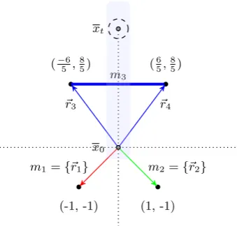
Figure 1: Bounded-rate multi-mode system with
three modes and two variables.
for bounded-rate multi-mode systems. We show that the problem is co-NP complete. Moreover, we show that it is fixed parameter tractable, i.e., if the number of dimensions is fixed, then the robust reachability problem can be solved in polynomial time.
Our existence proofs are constructive: in case of a positive answer, we can also give a dynamic schedule that, given a tolerance levelε>0, guarantees reachability of an open ball of ε radius around the target state in finitely many steps. It is then simple to extend these results to different path planning problems. We discuss the extension of the robust reachability problem to motion planning, and exploit our results to provide an alternative and simpler proof for the decidability of the robust schedulability problem. We also show that this problem can be solved in polynomial time for systems with fixed dimension, improving the result [4] where authors only give a polynomial algorithm to decide 2-dimensional systems. We notice that these results can be combined to stable reachability, where the goal is to first reach anε ball around a target, and then stay in this ball for ever.
Example 1. An example of a bounded-rate multi-mode system with two variables, say x and y, and three modes m1, m2, and m3, is given in the Figure 1. Modesm1 and m2 are precise, while mode m3 is uncertain, and environ-ment can give any rate vector that is a convex combination of rate vectors ~r3 and ~r4. The safety set is given as the blue rectangle. The reachability problem here is to decide whether, for everyε >0, controller has a sequence of time delays and choice of modes such that no matter what rate is given by the environment the system reaches a state inε -neighborhood ofxt. The schedulability problem asks whether
the scheduler has an infinite non-Zeno sequence of choices of modes and time delays such that the system always stays within the safety set, while stable reachability problem asks for a strategy to first reach anε-neighborhood ofxtand then
to stay in that neighborhood using a non-Zeno strategy.
We also consider the reachability problem with minimum dwell-time requirement and show that in the absence of the safety set the problem is undecidable for arbitrary bounded-rate multi-mode systems, but turns out to be decidable for
systems with non-negative rates. We also study the prob-lem of the existence of discrete control where controller is re-quired to choose modes at times multiple of a given sampling rate. We show that the reachability problem is EXPTIME-complete for this class of controllers. Finally, we show that adding very simple structure to bounded-rate multi-mode systems by introducing clock variables (variables with pre-cise uniform rates in each mode)—that appear as guards on the transitions and can be reset on the discrete transitions— leads to undecidability of the robust reachability problem.
Our algorithm can be combined with algorithms to ex-plore non-convex high-dimensional spaces, such as rapidly exploring random tree (RRT) algorithm [11], to yield robust control for such systems. Intuitively, RRT algorithm can return a path from the source to the destination by random exploration of the state space, which can be robustly fol-lowed by repeated applications of our algorithm in context of systems modeled as bounded-rate multi-mode systems.
For a review of related work on constant-rate multi-mode systems we refer the reader to [4, 5]. Le Ny and Pappas [12] initiated work on the sequential composition of robust con-troller specifications. In this light, our results can be under-stood as an effort to analyze complexity of this problem for the system of relatively simple dynamics. There is a huge body of work on path-following and trajectory tracking of autonomous robots under uncertainty. For a detailed sur-vey we refer the reader to [1]. There is a vast literature on decidable subclasses of hybrid automata [2, 7]. Most no-table among these classes are initialized rectangular hybrid automata [9], two-dimensional piecewise-constant derivative systems [6], and timed automata [3].
The paper is organized as follows. We begin by formal def-inition of the problem in the next section, followed by the proof of our key result in Section 3. We present some appli-cations of our main algorithm to solve schedulability, stable reachability, and path following problems in Section 4. In Section 5 we present results regarding bounded-rate multi-mode systems with discrete controller and dwell-time re-quirements. We conclude the paper by discussing results on generalized model in Section 6.
2.
ROBUST REACHABILITY PROBLEM
Prior to formally introducing the robust reachability prob-lem for multi-mode systems, we set the notation used in the rest of the paper and recall some standard results.
2.1
Preliminaries
Points and Vectors. LetRbe the set of real numbers. We represent the states in our system as points inRn that is equipped with the standard Euclidean norm k · k. We denote points in this state space byx, y, vectors by~r, ~v, and thei-th coordinate of pointxand vector~rbyx(i) and~r(i), respectively. We write~0 for a vector with all its coordinates equal to 0; its dimension is often clear from the context. The distancekx, ykbetween pointsxandyis defined askx−yk.
Boundedness and Interior. We denote anopen ballof radiusd∈R≥0centered atxasBd(x)={y∈Rn : kx, yk< d}. We denote a closed ball of radiusd∈R≥0 centered at xas Bd(x). We say that a setS ⊆Rn isboundedif there exists
Convexity. A pointxis aconvex combinationof a finite set of pointsX={x1, x2, . . . , xk}if there areλ1, λ2, . . . , λk∈
[0,1] such thatPk
i=1λi= 1 andx=
Pk
i=1λi·xi. Theconvex hull ofX is the set of all points that are convex combina-tions of points inX. We say thatS ⊆Rnisconvexiff, for allx, y∈Sand allλ∈[0,1], we haveλx+ (1−λ)y∈Sand moreover,S is aconvex polytopeif it is bounded and there existsk∈N, a matrixAof sizek×n and a vector~b∈Rk such thatx∈S iffAx≤~b.
A pointxis avertex of a convex polytopeP if it is not a convex combination of two distinct (other thanx) points in P. For a convex polytopeP we writevert(P) for the finite set of points that correspond to the vertices ofP. Each point inP can be written as a convex combination of the points invert(P). In other words,P is theconvex hull ofvert(P).
2.2
Multi-Mode Systems
A multi-mode system is a hybrid system, or rather a switched system, equipped with finitely many modes and finitely many real-valued variables. A configuration is de-scribed by the values of the variables. These values change as time elapses at the rates determined by the modes be-ing used. The choice of the rates is nondeterministic, which introduces a notion of adversarial behavior.
Definition 1 (Multi-Mode Systems). A multi-mode system is a tuple H = (M, n,R) where: M is the finite nonempty set of modes,nis the number of continuous vari-ables, and R: M →2Rn is the rate-set function that, for
each modem ∈M, gives a set of vectors. We often write ~r∈mfor~r∈ R(m)when Ris clear from the context.
A finite run of a multi-mode system H is a finite se-quence of states, timed moves, and rate vector choices%=
hx0,(m1, t1), ~r1, x1, . . . ,(mk, tk), ~rk, xki s.t., for all 1≤i≤ k, we have~ri ∈ R(mi) and xi =xi−1+ti·~ri. For such a
run%we say thatx0is thestarting state, whilexkis itslast
state. An infinite run is defined in a similar manner. We writeRunsandFRunsfor the set of infinite and finite runs ofH, andRuns(x) andFRuns(x) for the set of infinite and finite runs ofHthat start fromx.
An infinite runhx0,(m1, t1), ~r1, x1,(m2, t2), ~r2, . . .iisZeno ifP∞i=1ti <∞. Given a setS ⊆Rnof safe states, we say that a runhx0,(m1, t1), ~r1, x1,(m2, t2), ~r2, . . . ,(mk, tk), ~rk, xki
isS-safe ifxi∈S for all 0≤i≤k; and for all 0≤i<kwe have
thatxi+t·~ri+1 ∈S for all t∈[0, ti+1], assumingt0 = 0. Notice that, ifSis a convex set andxi∈Sfor alli≥0, then
this holds iff xi ∈ S for all 0≤i≤k. Sometimes we simply
call a run safe when the safety set is clear from the context. We formally give the semantics of a multi-mode systemH
as a turn-based two-player game between two players, sched-uler andenvironment, who choose their moves to construct a run of the system. The system starts in a given starting statex0 ∈Rn. At each turn, the scheduler chooses a timed move, a pair (m, t) ∈ M×R>0 consisting of a mode and a time duration, and the environment chooses a rate vector ~r∈mand as a result the system changes its state fromx0 to the state x1 = x0 +t·~r in t time units following the linear trajectory according to the rate vector~r. From the next state, x1, the scheduler again chooses a timed move and the environment an allowable rate vector, and the game continues forever in this fashion. The focus of this paper is on robustreachabilityproblem where, given a starting state x0, a target vertexxt, a bounded and convex safety setS
and tolerance ε >0, the goal of the scheduler is to visit a state in an open ball of radiusεcentered atxt via anS-safe
run. The goal of the environment is the opposite.
Given a bounded and convex safety set S and tolerance ε>0, we define therobust reachability objectiveWS
Reach(xt, ε)
as the set of infinite runs ofHthat visit a state inBε(xt). In
a reachability game the winning objective of the scheduler is to make sure that the constructed run of a system belongs to WS
Reach(xt, ε), while the goal of the environment is the
opposite. The choice selection mechanism of the players is typically defined as strategies. Astrategyσof the scheduler is functionσ:FRuns→M×R≥0 that gives a timed move for every history of the game. A strategyπof the environment is a functionπ:FRuns×(M×R≥0)→Rnthat chooses an allowable rate for a given history of the game and choice of the scheduler. We write Σ and Π for the set of strategies of the scheduler and the environment, respectively.
Given a starting statex0and a strategy pair (σ, π)∈Σ×Π we define the unique runRun(x0, σ, π) starting fromx0 as
Run(x0, σ, π) =hx0,(m1, t1), ~r1, x1,(m2, t2), ~r2, . . .i
where, for alli≥1, (mi, ti) =σ(hx0,(m1, t1), ~r1, x1, . . . , xi−1i) and ~ri = π(hx0,(m1, t1), ~r1, x1, . . . , xi−1, mi, tii) and xi = xi−1+ti·~ri. The scheduler wins the game if there is a σ ∈ Σ such that, for all π ∈ Π, we get Run(x0, σ, π) ∈
WS
Reach(xt, ε). Such a strategyσ iswinning. Similarly, the
environment wins the game if there isπ∈ Π such that for all σ ∈ Σ we have Run(x0, σ, π) 6∈ WReachS (xt, ε). Again, π is called winning in this case. If a winning strategy for scheduler exists, we say that the statextisε-reachable from
the statex0 for given safety setS and toleranceε. We also say that the statext isrobustly reachablefromx0 if it isε -reachable for allε >0. The following is the main algorithmic problem studied in this paper.
Definition 2 (Robust Reachability). Given a multi-mode systemH, a convex safety setS, a starting statex0∈ int(S), and a target statext ∈int(S), decide whether xt is
robustly reachable from x0.
To algorithmically decide the robust reachability problem, we need to restrict the range of R and the domain of the safety setS in a robust reachability game on a multi-mode system. The most general model that we consider is the bounded-rate multi-mode systems (BMS).
Definition 3 (Bounded-Rate Systems). A bounded-rate multi-mode system (BMS)is multi-mode system H = (M, n,R) such that R(m) is a convex polytope for every m∈M. We also assume that the safety setS is specified as a convex polytope.
For every modemi∈M of aBMSwe assume an arbitrary
but fixed ordering on the vertices of R(m). By exploiting the notations slightly, it allows us to writeR(mi)(j) for the
rate vector corresponding toj-th vertex of modemi. When
there is no confusion, we also writeR(i)(j) forR(mi)(j).
In our proofs we often refer to another variant of multi-mode systems, in which there are only a fixed number of different rates in each mode (i.e.,R(m) is finite for allm∈
m0,0
m0,1 m1,0
(a) Constant-Rate
m0,0
m0,1 m1,0
(b) Bounded-Rate
m0,0
m0,1 m1,0
[image:4.595.58.288.51.142.2](c) Multi-Rate
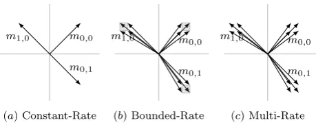
Figure 2: Restricted Multi-mode Systems
to refer to the unique element of the set R(m) in a CMS. The concepts related to the robust reachability games for BMSandMMSare already defined for multi-mode systems. Similar concepts also hold forCMSbut with no real choice for the environment. Examples ofCMS,BMS, andMMSare shown in Figure 2.
We say that a CMS H = (M, n, R) is an instance of a multi-mode systemH= (M, n,R) if for every m ∈M we have that R(m) ∈ R(m). For example, the CMS shown in Figure 2.(a) is an instance of BMSin Figure 2.(b). We denote the set of instances of a multi-mode system H by [[H]]. Notice that for aBMSH, the set [[H]] of its instances is uncountable (unless theBMSis aCMS), while for anMMSH
the set [[H]] is finite, and exponential in the size ofH. We say that anMMS(M, n,R0) is theextreme-rate MMSof aBMS (M, n,R) ifR0
(m) =vert(R(m)). TheMMSin Figure 2.(c) is the extreme-rateMMS for theBMS in Figure 2.(b) We writeExt(H) for the extreme-rateMMSof theBMSH.
The following theorem is the key observation of the paper.
Theorem 1. Given aBMSH= (M, n,R), convex safety setS, starting statex0∈int(S)and target statext∈int(S),
the target statextis robustly reachable if and only if for every CMSin[[Ext(H)]]the statext is reachable fromx0.
Alur et al. [5] presented a polynomial-time algorithm to decide if a state xt is reachable from a starting state x0 forCMS. In particular, for starting and target states in the interior of the safety set, they characterized a necessary and sufficient condition.
Theorem 2 ([5]). The scheduler has a winning strat-egy in aCMS(M, n, R), with convex safety setS and start-ing state x0 ∈ int(S) and target state xt ∈ int(S), if and
only if there is~t∈R|≥M0| satisfying:
x0+
|M| X
i=1
R(i)(j)·~t(i) =xt for1≤j≤n. (1)
Notice that in such a case controller has a strategy to reach the target state precisely. The intuition behind Theorem 2 is that the scheduler has a winning strategy if and only if it is possible to reach the target state from the starting state in using a combination of the rate vectors.
Using Theorems 1 and 2 it follows that the robust reach-ability problem is in co-NP. By reducing the validity check-ing problem of propositional logic formulas in DNF, we show that the robust reachability problem forBMSis indeed com-plete the class co-NP. On a positive side, we show that the robust reachability problem forBMSand CMSis fixed pa-rameter tractable, i.e. it is polynomial for fixed number of variables. It brings us to our next key result.
Theorem 3 (Complexity). The robust reachability prob-lems forBMSandCMSare co-NP complete. However, it is fixed parameter tractable with fixed number of variables.
3.
DECIDABILITY AND COMPLEXITY
This section is dedicated to the proofs of Theorem 1 and Theorem 3.
3.1
Proof of Theorem 1
We prove Theorem 1 by showing that the condition is necessary and sufficient in the following two lemmas.
Lemma 4. Given a BMS H, safety set S, starting state x0 ∈ int(S) and target state xt ∈ int(S), the target state
is not robustly reachable if there exists aCMS(M, n, R) in [[Ext(H)]]for whichxt is not reachable fromx0.
Proof. From Theorem 2, we have that an interior point xtofSis reachable iff it is in the conical hull of rates in the
CMS. LetKdenote this connical hull. Note thatKis closed and that, by our assumption,xt∈ K/ . This implies that the
distance ε = infx∈Kkxt, xk between xt and K is positive.
Consequently, B(xt) and K are disjoint. It follows that
when the environment follows the strategy to choose the rate R(m) when presented with a mode m, then the controller cannot reach anball aroundxt.
Lemma 5. Given a BMS H, safety set S, starting state x0 ∈int(S) and target statext ∈int(S), the target state is
robustly reachable if for all CMS(M, n, R) in [[Ext(H)]]the statext is reachable fromx0.
We give a constructive proof of this lemma by constructing an algorithm (Algorithm 1) giving a strategy of the player to reachB(xt) for a given >0.
Before we elaborate on the working of the algorithm, we need to explain the idea of projections. In our algorithms we sometimes represent a point x∈ Rn by explicitly defining its projection towards the direction vector~v=xt−x0 and (small) projections towards extreme rate vectors of various modes.
Definition 4 (Projection). Given a BMS(M, n,R) we say that a tuple(λ, π)is a projectionof a pointx, where λ ∈ R≥0 is the projection towards ~v and π : N×N → R≥0 is the projection towards extreme rate-vectors of var-ious modes, such that π(i, j) is the projection towards j-th vertex of the rate polytopeR(mi), if:
x=λ·~v+
|M| X
i=1
|vert(R(mi))| X
j=1
π(i, j)· R(i, j).
Notice that such projections are often not unique. We write the(λ0, π0)for the projection such thatλ0= 0andπ0(i, j) = 0for alli, j. Given a projectionP = (λ, π)of a statexwe say that π(i, j) is the contribution of the jth vertex of the
rate polytope of modemi. We also say that a vertexR(i, j)
does not contribute in a projection P if π(i, j) = 0, while we say that a mode does not contribute in a projection P if π(i, j) = 0holds for all cornersjofR(mi).
Given a tolerance level of , the strategy for the player to reachB(xt) is given by Algorithm 1. A feature of the
the mode that the player chooses. Depending on the choice of the environment, the current point is updated. This pro-cess goes on until an ball around xt is reached.
Algorithm 1:Dynamic reachability algorithm
Input: BMMSH, starting statex0, tolerance level Output: Reachability Algorithm
1 B:= max
m∈M~r∈Rmax(m)k~rk; 2 x:=x0, the current point;
3 ~v:=xt−x0, the reachability direction;
4 γ1:= the shortest distance ofx0 from borders ofS; 5 γ2:= the shortest distance ofxt from borders ofS;
6 τ := min(/2, γ1, γ2)/(B|M|);
7 σ:= an array, one element for eachCMSF in [[Ext(H)]] s.tσ(F) =~ts.t. ~tis a solution for theCMSF for reachability to~v;
8 ProjectionP = (λ0, π0) ; 9 whilekx−xtk> do
10 P,m=nextMode(P,~v,σ); 11 ~r=senseCurrentRate(x,m,τ); 12 x=x+τ~r;
13 P =updateProjection(P,m,~r);
Algorithm 2:nextMode(P,~v,σ)
Input: ProjectionP, reachability direction~v, reachability solution arrayσ
Output: ProjectionP, modem 1 whiletrue do
2 if there exists modemi having zero contribution to
Projection P then
3 returnP,mi;
4 else
5 R(mi) :=vert(R(mi))(j) such that
vert(R(mi))(j) has non-zero contribution toP
for eachi;
6 CMSF:= (M, n, R) is the corresponding instance ofH;
7 P=reduceComp(F, σ(F), P);
The job of nextMode function is to nullify the contri-bution of a mode mby expressing the point in a different way. It calls uponreduceCompfunction described in Algo-rithm 3 to achieve this. The correctness of the AlgoAlgo-rithm 3 follows from the following proposition.
Proposition 6. Every non-negative linear combination of rates of a CMSF= (M, n, R)∈[[Ext(H)]]that is reach-able to~v can be written as the sum of a non-negative com-ponent along~vand a non-negative linear combination of the rates where contribution of one of the rates is0.
Proof. Given a CMS F = (M, n, R) as an instance of [[Ext(H)]], we have
~ v=
|M| X
i=1
σ(F)(i).R(mi) (2)
Given any non-negative linear combination of vectors inR,
P|M|
i=1ciR(mi),ci≥0, letk= arg mini,σ(F)(i)>0(ci/σ(F)(i)).
Algorithm 3:reduceComp(F, σ(F), P)
Input: CMSF = (M, n, R), solution time vector for theCMSσ(F), current ProjectionP = (λ, π)
Output: ProjectionP0= (λ0, π0) s.t. contribution of one of the rates inF has been nullified 1 (λ0, π0) = (λ, π);
2 k:= arg min
i,σ(F)(i)>0
(π(i, R(i))/σ(F)(i));
3 λ0=λ+π(k, R(mk))/σ(F)(k);
4 foriin{1,2, . . . ,|M|}do 5 π0(i, R(i)) =
π(i, R(i))−(π(k, R(k))∗σ(F)(i))/σ(F)(k);
6 return (λ0, π0);
Algorithm 4:updateProjection(P, m, ~r)
Input: current ProjectionP= (λ, π), modemi, rate~r Output: ProjectionP= (λ0, π0) with ratertaken for
timeτ 1 (λ0, π0) = (λ, π);
2 ~r=P|jvert=1 (R(mi))|θjvert(R(mi))(j), the convex
combination of vertex of the rate polytope of modemi;
3 forjin{1,2, . . . ,|vert(R(mi))|}do
4 π0(i, j) =θj∗τ;
5 return (λ0, π0);
The following calculations show that every non-negative lin-ear combination of rates of a CMS F = (M, n, R) that is reachable to~vcan be written as the sum of a non-negative component along~v and a non-negative linear combination of the rates where contribution of one of the rates is 0. For clarity,σ(F)(i) has been written asσibelow.
|M| X
i=1
ciR(mi) = |M| X
i=1 (ci−
ckσi σk
+ckσi σk
)R(mi)
=
|M| X
i=1 (ci−
ckσi σk
)R(mi) + |M| X
i=1 ckσi
σk R(mi)
=
|M| X
i=1 (ci−
ckσi σk
)R(mi) + ck σk
|M| X
i=1
σiR(mi)
=
|M| X
i=1 (ci−
ckσi σk
)R(mi) + ck σk ~v
The last step follows from Equation 2. Note that, since k = arg mini,σi>0(ci/σi), we have thatci−
ckσi
σk ≥0 holds
for eachiand = 0 holds fori=k.
This explains the working of Algorithm 3. We say that the contribution of R(mk) is consumed in this process. Every
invocation of Algorithm 3 consumes at least one corner of one of the modes inM. Hence, it guarantees that after some finite iterations, some mode will be consumed in the process. This proves the termination of Algorithm 2.
Proposition 7 (Safety). All the states visited during an execution of Algorithm 1 are strictly inside the safety set.
point reached at any step in the algorithm,x, can be written as the sum of a non-negative component along~vand small components along some rate in each of the modes. Formally,
x = λ~v+
|M| X
i=1
ti~ri, (3)
whereλ≥0,~ri∈ R(mi), 0≤ti≤τ for all modesmi∈M.
We prove this by induction on the number of steps. The initial pointx0 = 0 is trivially written in the above form withλ= 0, ti= 0 and ri, any rate vector in modemi for
alli. If, afterjsteps,x=λ~v+P|i=1M|ti~riwithλ≥0, ti≥0
for all i, then Algorithm 2 ensures thatx can be written in an alternative way such that the contribution of some mode mk is 0 in x. In this process, λ is non-decreasing
and the contribution of other modes is non-increasing but always≥0. This providesx=λ1~v+Pi∈[|M|]\{k}t0i~r
0 i with λ1≥λ,0≤t0i≤ti. The mode chosen by the player in this
step ismk and the time chosen isτ, the new point reached
isx0=x+P|iM=1|t0i~r 0
i, wheret 0
k=τand~r 0
kis the rate chosen
by the environment in mode mk. So, we again havex0 in
the form specified by Equation 3.
|x−λ~v| = |
|M| X
i=1 tiri| ≤
|M| X
i=1
|tiri|
≤
|M| X
i=1 τB≤
|M| X
i=1
min(/2, γ1, γ2)
|M| = min(/2, γ1, γ2).
We have used the value ofτ defined in Algorithm 1. The last equation also shows that the current point is inside a ball of radius/2 from the pointλ~v.
We now prove that λ ≤ 1 +/(2k~vk). We prove this by induction on the number of steps. Initially, λ = 0 ≤
1 +/(2k~vk). Let xj and xj+1 be the point reached after j and j+ 1 steps, respectively. Afterj steps, ifλj ≤1 + /(2k~vk) and we are not inside an ball around xt, then
by geometry, λj ≤1−/(2kv~k). Let λj and λj+1 be the respective projection along direction~v. Suppose, some rate ~ris taken for timeτ. Then,
kxj+1−xjk=kτ rk ≤τkrk ≤τB≤ 2|M|
So, successive points differ by a distance of at most/2|M| ≤
/2 and they are centered aroundλj~vandλj+1~vin a ball of radius/2. Sincekλj+1v~−λj~vk ≤we have that
λj+1≤λj+
k~vk≤1 +
(2k~vk)
The last step follows from λj ≤ 1−/(2k~vk) as argued
already. So, we have proved by induction that λ ≤ 1 + /(2k~vk). Therefore, at any step in the algorithm,λ~v is a convex combination of x0 and xt+~v/(2k~vk). Therefore,
a ball of radius min(/2, γ1, γ2) lies completely inside the safety setS. This follows from the definition ofγ1 andγ2. So, the algorithm is safe.
Proposition 8 (Termination). The Algorithm 1 al-ways terminates.
Proof. We show that the algorithm terminates in finitely many steps by demonstrating the progress towards the tar-get state. We say thatτof modemis pumped in Projection
P at stepjof the algorithm, if the player chooses modem at step j. We show that there exists δ > 0 such that, in every|M|+ 1 steps of the algorithm, the variableλof the current point P increases by at leastδ. Consider |M|+ 1 consecutive runs of the algorithm. Since we pump a mode at every step of the algorithm, there is a modemi, which was
chosen twice for pumping. This implies that at leastτ ofmi
was consumed inn steps. So, at leastτ /|vert(R(mi))|was
consumed by some vertexR(mi)(j) ofR(mi). EveryCMS
with R(mi) = R(mi)(j) guarantees a fixed increase δ1 in λ forτ /|vert(R(mi))|consumed of cornerR(mi)(j), since
the solution vectorσ(F) for everyCMSF is fixed. Hence,δ equals the mininum ofδ1 over all vertices of all modes is the least increase in λ. This is the minimum increase inn+ 1 steps of the algorithm. Hence, progress is proved.
Now, we show termination. Progress ofδin every|M|+ 1 iterations along with the condition λ ≤ 1 +/(2k~vk) and increase in λ bounded by in every step guarantee that, after some finite iterations, 1−/(2k~vk)≤λ≤1 +/(2k~vk), in which casekx−λ~vk ≤/2 impliesx∈B(xt).
The proof of Lemma 5 is now complete.
3.2
Proof of Theorem 3
With the two lemmas in place, we can proceed with prov-ing the main complexity results. We start with the positive result that states that the problem is tractable in practice.
Theorem 9. The reachability problem forBMSandMMS
is fixed parameter tractable, where the parameter is the num-ber of variables. In particular, it is polynomial forBMSand
MMSwith fixed dimensiond.
Proof. We first observe that, for fixed dimensions, the number of extreme points per mode is polynomial in the size of the defining matrix. Thus,Ext(H) is polynomial inHfor BMSH.
For the sake of simplicity assume that the starting point is the origin and we wish to reach positionp.
From Lemmas 4 and 5, we can infer that the existence of a CMS ∈ [[Ext(H)]] for which p is not reachable from the origin is a necessary and sufficient criterion for refuting reachability. By Theorem 2, for aCMSC the statepis not reachable from the origin iff it is not in the conical hull of its vertices. This is the case, iff there is a hyperplane through the origin that does not containp, such that the half-space withoutpit defines contains all vertices ofC.
Letk≤dbe the dimension of the hull ofvert(C). We now distinguish two cases. First, assume thatpis not in the hull ofvert(C). In order to validate this, we can simply takek < dvectors ofC and validate that they are a basis of vert(C).
Now we assume thatpis in the hull ofvert(C). We now work in vert(C). There are k−1 vectors in vert(C) that define a hyperplane in this hull, s.t. the half-space without pit defines contains all vertices ofC. 1
The next observation we make is that
– the k < dspanning vectors used from extreme points of different modes are sufficient to establish the first case in polynomial time for theMMS, because one can cheaply check that all other modes contain a vector in the space they span, whilepis not a linear combination of them, and
– the k−1 spanning vectors used from extreme points of different modes are sufficient to establish the second case in polynomial time for theMMS, because one can cheaply check that p is not a linear combination of them, and all other modes contain a vector in the k dimensional space spanned by them andp, andpdoes not enter positively in the linear combination.
Thus, it suffices to perform cheap (polynomial) tests for sets of less than d vectors. The number of these sets is polynomial for fixedd.
Theorem 10. The reachability problem forBMSandMMS are co-NP complete.
Proof. The inclusion in co-NP is implied by Lemma 4: to refute reachability, it is enough to guess a CMSC from [[H]] of anMMS or [[Ext(H)]] from aBMS H and to verify that the target is not reachable fromC. The verification can be performed in polynomial time from Theorem 2.
We show co-NP hardness by reducing the validity checking of propositional logic formulas in DNF, where each clause is a conjunction of three literals, which refer to different propositions. We give a full proof forBMS.
Given such a formulaϕ withm clausesD1, . . . , Dm and n ≥ 3 variables x1, . . . , xn, we construct a BMS with less
than 7m+ 2n+ 3 modes and n+ 3 variables. We name nof these variables the propositions, x1, . . . , xn, and there
are three further variables, y1, y2, y3, which are intuitively manipulated in three different stages of a game. Initially, all variables are 0, and the goal is to reach a state, where y1=y2= 1,y3=n−3, andx1 =x2 =· · ·=xn= 0. The
safety set for all variables is the interval [-1,1].
Givenϕ=D1∨D2∨· · ·∨Dm, where eachDihas 3 literals,
we consider subclauses ofD1, . . . , Dm. EachDi has 6
non-empty subclauses. Considering the non-empty clause as well, we obtainl≤7m+ 1 clausesD1, . . . , Dm, Dm+1, . . . , Dl. Note
that we do not changeϕ, we only need the new clauses for technical reasons. LetN(Di) ={j|xjor¬xjoccurs inDi}
for alli= 1, . . . , l.
TheBMShas only one nondeterministic mode,me, which
is also the initial mode. Intuitively, the environment chooses the valuation of the variables in this mode. OurBMSallows all rate vectors with R(me)(xi) ∈ [−1,1] for 1 ≤ i ≤ n,
R(me)(y1) = 1, andR(me)(y2) = R(me)(y3) = 0.
Intu-itively, the environment tries to select a valuation of the variables x1, . . . , xn that does not satisfy ϕ in this mode,
where the value 1 refers to ‘true’ and −1 refers to ‘false’. me is the only mode withy16= 0. Given the goal, the con-troller must be in the modeme for exactly one time unit.
For each clause in the extended set of clauses (i.e., for i= 1, . . . , l), ourBMShas a clause mode,mi. We have:
– R(mi)(xj) = 1 if¬xjoccurs inDi,
– R(mi)(xj) =−1 ifxj occurs inDi,
– R(mi)(xj) = 0 for allj /∈N(Di), and
– R(mi)(y1) =R(mi)(y3) = 0, andR(mi)(y2) = 1.
Intuitively, the scheduler selects a clause fromD1, . . . , Dm,
and resets the values of the three variable occurring in the clause to 0. The role of the additionall−m clauses is to account for the capability of the environment to select values different from −1 and 1. The clause modes are the only modes withy2 6= 0. Given the goal, the scheduler must be in clause modes for exactly 1 time unit.
For each of variablexi, ourBMShas two correction modes, m+i andm
−
i , and one empty correction nodem0. We have:
– R(m+i)(xi) = 1,R(m+i)(xj) = 0 for allj6=i,
R(m+
i)(y1) =R(m
+
i)(y2) = 0, andR(m
+
i )(y3) = 1,
– R(m0)(xi) = 0, for all i = 1, . . . , n, R(m0)(y1) =
R(m0)(y2) = 0, andR(m0)(y3) = 1, and
– R(m−i )(xi) =−1,R(m−i)(xj) = 0 for allj6=i,
R(m−i )(y1) =R(m+
i )(y2) = 0, andR(m −
i)(y3) = 1.
Intuitively, the scheduler resets the values of the remaining n−3 variables, not covered by the clause, to 0 using these correction modes. The correction modes are the only modes with y3 6= 0. Given the goal, the scheduler must be in correction modes for exactlyn−3 time units.
We first observe that the reachability problem is poly-nomial in ϕ. Next, we convince ourselves that the goal is reachable ifϕis valid.
In this case, the scheduler first stays in modeme for one
time unit. It then identifies an i ∈ {1, . . . , m} such that, for allj ∈ N(Di), ifxj >0 then xj is a literal of Di and
if xj < 0 then ¬xj is a literal of Di. The scheduler can
then apply the clause modes for Di and/or its subclauses
for together one time unit such that, after this time unit, xj= 0 holds for allj∈N(Di).
Next, the scheduler can apply, for all j /∈ N(Di) the
correction mode m+j for xj time units if xj > 0 or m−j
for −xj time units if xj < 0. Given a clause Di,
j ∈ {1, . . . , n} |j /∈N(Di) =n−3, this brings us to a point
withx1 =. . . =xn = 0,y1 =y2 = 1, and y3 ∈[0, n−3]. From there, we can apply m0 fory3+ 3−n time units to reach the goal.
Finally, we have to check that, ifϕis not valid, then the goal is not reachable. To see this, note that thememust be
scheduled for exactly one time unit. The environment can therefore select a configuration that does not satisfy ϕand choose rates−1 for ‘false’ and 1 for ‘true’ for this configu-ration each timem0is scheduled.
Now let us assume that the environment follows this pol-icy, but the goal is reached. First we observe that the sys-tem must be for 1 time unit inme, for 1 time unit in clause
modes, and forn−3 time units in correction modes. Clearly, some clause modemiis used forttime units, witht∈[0,1].
Note that, if Di refers to a clause that is satisfied by the
configuration, then Di has at most two literals. Now we
observe that
– when considering the effect of the 1 time unit inme,
we havePn
j=1|xj|=n,
– when considering the 2 time units the system is inme
or a clause modemi, we havePnj=1|xj| ≥n+t−3 (no Diexists satisfying the chosen assignment, thust >0)
– after the completen−1 time units of the run, we have
Pn
j=1|xj| ≥t >0.
This provides a contradiction to having reached the goal. The proof can easily be extended to MMS, however we have to overcome the exponential size of the extreme-rates forme. In order to achieve this, we splity1 intonvariables y1
1, . . . , yn1 and replaceme bynmodes m1e, . . . , mne. R(mie)
has two points, whereyi
1 = 1, xi ∈ {−1,1} and all other y2 =y3 = xj = 0 for all j 6=i. For the goal, we require y11 =. . . =yn1 = 1 instead of y1 = 1. The only change is that the environment now selects the values for the atomic propositions successively instead of concurrently.
4.
APPLICATIONS
In this section, we show how to apply our results for
– robust schedulability—to decide if, for allε >0, there is a non-Zeno control strategy, which guarantees that the system stays in anεball around the starting point;
– robust stability—to decide if, for all ε >0, there is a non-Zeno control strategy, which guarantees that the system reaches an εball around the target point and then never leaves it again (possibly while staying in a convex safety set where the starting vertex and the targetxtare inner points); and
– robust path following—to decide if, for all ε > 0, a given path can be followed withεprecision.
4.1
Robust Schedulability
For ease of notation, we assume w.l.o.g. that this point is the origin0, and we assume w.l.o.g. thatε <1. The problem has been studied before in [4], but the proof we provide here is much simpler.
Robust schedulability can be derived from robust reach-ability by first tweaking the reachreach-ability problem slightly, such that one execution guarantees to stay within aε-ball while consuming at least one time unit.
The central idea for adjusting a system withd variables x1, . . . , xd is to add one variable, c, that serves as a clock.
In all rates of all modes, the rate in which this new vari-able progresses is 1. Next, we define the safety set asS =
{(x1, . . . , xd, c) | ∀i≤ d.2d|xi| ≤ ε}, or any other convex
set that does not constrain the values of c and that con-straints the values of the remaining variables to be in the εball around0. We now consider the problem of reaching the pointxt withx1=. . .=xd= 0 andc= 1 withε
preci-sion. First, when projecting away the clockc, the safety set alone guarantees to be in anε ball around 0, and second, the value ofcmust be greater than 1−ε, which implies with the constant rate 1 that at least 1−εtime units have past. Ifxtis not robust reachable from0, then there is anε, for
whichBε(xt) cannot be reached. Thus, no strategy exists
to keep the system in an ε/d ball around 0 for one time unit, as this control strategy could be applied to reach the ε ball around xt. If, however, xt is robust reachable from 0, then we can repeatedly apply such a strategy, first for ε1, then forε2, and so forth, whereεi= 2−iε. It is easy to
see that the resulting composed strategy is non-Zeno, as all components are finite and at least one time unit passes in each component. It is also easy to see that the error can at most add up, such that one always stays in anεball around the starting point.
4.2
Robust Stability
Obviously, reachability toxtand robust schedulability are
prerequisites for robust stability. To see that they are also sufficient, we assuming w.l.o.g. that the ballBε(xt) is
con-tained in the safety set S. It then suffices to reach an xt
with precisionε/2, and then to follow a robust reachability strategy to stay in anε/2 ball around the point reached.
4.3
Robust Path Following
To robustly follow a piecewise linear path with precision ε, we can simply follow the first piece with precisionε1, the second with ε2, and so forth, where εi = 2−iε. Following
a piecewise linear path is therefore possible with arbitrary precision if each segment can be followed individually with arbitrary precision. Conversely, if one of these segments can-not be followed with arbitrary precision, then, obviously, the complete path cannot be followed with arbitrary precision. Note that the necessary and sufficient criterion extend to infinite paths composed of an infinite sequence of segments. Following a segment with arbitrary precision is essentially a robust reachability problem. If the endpoint of the seg-ment is robustly reachable from its starting point, then we can, for a given ε, define an convex set, where each point has distance at most ε to the segment, and that contains theε/2 ball around the goal. We then run Algorithm 1.
This can be extended to piecewise smooth (continuously differentiable) paths that can be approximated arbitrarily closely by a (possibly infinite) sequence of segments, where the endpoint of each segment is reachable from its starting point. This is the case iff the derivation satisfies everywhere (where defined) the condition for robust reachability.
5.
MINIMUM DWELL-TIME CONDITION
In this section, we consider an extension of robust reach-ability to robust reachreach-ability with or without dwell-time or discrete sampling. We assume w.l.o.g. that the minimal dwell-time or the sampling rate, respectively, is 1.
Theorem 11. The robust reachability problem with dwell-time requirement is decidable forBMSwhere all rate vectors are positive.
Proof. W.l.o.g assume that the starting state in0 and the target state isxt. Notice that since all the rate vectors
are positive, and every mode should be taken for at least 1 time-unit, there is a boundK such that the target state is not reachable is it is not reachable in K steps. (K is easy to compute.)
For robust reachability under bounded steps one can write a formula in first-order theory of reals. Now the decidability of the robust reachability with dwell-time requirement for BMSwith positive rate vectors follows from the decidability of the first-order theory of reals.
Proof. We prove the result by a reduction from count-down games [10]. A countcount-down game is a tupleG= (N, T, (n0, B0)), whereN is a finite set of nodes,T ⊆N×N>0×N a set of transitions, and (n0, B0) ∈ N×N>0 is the initial configuration. The states of a countdown game, also called its configurations, areN× {0,1, . . . , B0}.
From any configuration (n, B), Player 1 chooses a num-berl∈N>0such that there exists a transition (n, l, n0)∈T with l ≤ C. Among all the available transitions of the form (n, l, n0), Player 2 selects an appropriate transition (n, l, n00)∈T. The new configuration is then (n00, C−l).
Player 1 wins when a configuration (n,0) is reached, and otherwise loses when a configuration (n, C) is reached where Player 1 cannot move. This is the case when, for all outgoing transitions (n, l, n0)∈T, we havel > C. W.l.o.g., we assume that there are no transitions (n, l, n)∈T for anyl∈N>0.
We now translate this game into a sampled robust reacha-bility problem, where the scheduler takes the role of Player 1, while the environment takes the role of Player 2.
The translation uses |N|+ 1 variables, a variable B re-flecting the remaining time budget and a variablenfor each element n ∈ N. Being in state (n, C) in the countdown game is intuitively represented byB=C,n= 1, andn0= 0 for all statesn0 6=n. The initial state is given by B=B0, n0 = 1, andn= 0 for all states n6=n0, i.e., by the state representing the initial configuration (n0, B0). The target is 0. The safety set is described by n ∈ [−0.5,1.5] for all n∈N andB∈[−0.5, B0+ 1].
The rates Player 1 selects become the modes of ourMMS. Thus, we have a modelfor eachl∈N>0, for which a
tran-sition (n, l, n0) ∈ T exists. The selection of the concrete transition by Player 2 becomes the choice of the mode by the environment. We therefore have, for a given mode l, one rate vector for each transition (n, l, n0)∈T, where the rates are n = −1, n0 = 1, B = −l, and n00 = 0 for all n00∈Nr{n, n0}.
Before we describe how to translate (winning) strategies, we first note that, from each translation of a configuration, the scheduler cannot make a move of length≥2. We first replace the target vertex by a the target regionB= 0. For this target region, there is a simple 1:1 translation between the moves and states for the countdown game and the reach-ability game, where each movelof Player 1 in the countdown game corresponds to the move (l,1) of the scheduler, while every move (n, l, n0) of Player 2 corresponds to the environ-ment selecting the corresponding rate.
To return to normal reachability, we add, for each node n∈N, a moden. This mode has only one rate, withB= 0, n=−1, andn0= 0 for all n0 6=n. Note that such a mode ncan only be applied from states that encode (n, C), and it can only be applied with duration 1. Once such a mode is applied, no further mode (of either type) can be applied in the future, as one variablen00 ∈N would afterwards have the value−1.
Now, a winning for Player 1 corresponds to winning strat-egy of the scheduler that ends by applying such a mode. This closes the proof for discrete sampling.
To expand this to dwell time, we sharpen the bounds for the safety set to n ∈ [−ε,1 +ε] for all n ∈ N and B∈[−ε, B0+ 1] for some ε < 8B1
0. Now, if Player 1 wins,
then the scheduler wins with the same strategy as above. If Player 2 wins, Player 1 is stuck in< B0 move pairs. When the environment mimics such a strategy (until Player 1 is
stuck) then the game reaches a position, where each vari-able value is in a 2(B0−1)ε < 14 range around the value it would have, had the scheduler played a duration of 1 for each move. Thus, the scheduler can, at most, play a “node mode”n ∈ N once, but it cannot reduce the value of B without leaving the safety region.
For discrete sampled controllers, we can easily show in-clusion inEXPTIMEby exploring the complete state-space. To do this, we can proceed in two steps. In a first step, we expand all values in the problem setting to integers by multiplying every value with the least common multiple of all denominators. (Note that this is a polynomial time re-duction.) Then we can be sure that all values are at integer points, and we can simply explore the complete state-space, which is exponential in the setting. As the lower bound is inherited from the previous proof, we get:
Corollary 13. The robust reachability problem with dis-crete sampling isEXPTIME-complete.
6.
GENERALIZED MODELS
In this section we consider generalization of theBMSby adding structure to the model using Alur-Dill style [3] clock variables, i.e. variables with rate 1 in every mode. In the resulting model only clock variables can occur on the transi-tions where they can be compared against natural numbers or can be reset. All other non-clock variables will behave like BMS. We show that forBMSwith clock the robust reacha-bility problem is undecidable forBMSwith 2 variables and 1 clock, andBMSwith 1 variable and 2 clocks.
We prove the undecidability of this problem by giving a re-duction from the halting problem for two-counter machines. Formally, a two-counter machine (Minsky machine) Ais a tuple (L, C) where: L={`0, `1, . . . , `n}is the set of
instruc-tions. There is a distinguished terminal instruction`ncalled
HALT.C={c1, c2}is the set of twocounters; the instruc-tionsLare one of the following types:
1. (incrementc)`i:c:=c+ 1; goto`k,
2. (decrementc)`i:c:=c−1; goto`k,
3. (zero-checkc)`i: if (c >0) then goto`k else goto`m,
4. (Halt)`n: HALT.
wherec∈C,`i, `k, `m∈L.
A configuration of a two-counter machine is a tuple (`, c, d) where`∈L is an instruction, andc, dare natural numbers that specify the value of counters c1 and c2, respectively. The initial configuration is (`0,0,0). A run of a two-counter machine is a (finite or infinite) sequence of configurations
hk0, k1, . . .i where k0 is the initial configuration, and the relation between subsequent configurations is governed by transitions between respective instructions. The run is a finite sequence if and only if the last configuration is the terminal instruction `n. Note that a two-counter machine
has exactly one run starting from the initial configuration. Thehalting problemfor a two-counter machine asks whether its unique run ends at the terminal instruction`n. It is well
known that the halting problem for two-counter machines is undecidable.
`i
(0,0)
N Z
{(0,0),(0,−100)}
Z
{(0,0),(0,−100)}
`2
`1 O
(0,100)
N (0,−1)
T (−1,0)
C
hk
1 x= 1?
x:= 0
x= 1? x:= 0
x= 1?, x:= 0 x= 1?, x:= 0
O (0,100)
T (−1,0) x= 1?, x:= 0
x= 1?, x:= 0
C
hk
2
x= 1 x:= 0
x= 1 x:= 0
x= 1?, x:= 0
x= 1?, x:= 0 x= 1? x:= 0
[image:10.595.59.295.51.251.2]x= 1? x:= 0
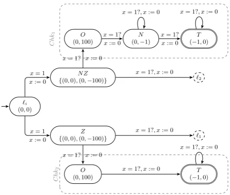
Figure 3: Simulation of Zero Check instruction
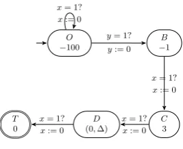
Proof. For the sake of simplicity of presentation we prove the undecidability of the exact reachability problem. The proof can be adapted to robust reachability case. Given a Minsky machine we construct a structured BMSHwith 2 variables and a single clock that is reset on every transi-tion. The clock is used in a simple way just to ensue that at each mode exactly 1 unit of time is spent by the con-troller. We use two variablesyand z to encode the values of the two countersc1 andc2, and one mode corresponding to each location of the Minsky machine. For each zero check instruction we further use five extra modes and a special target modeT depicted by a double circle. Our goal is to reach modeT withy=z= 0.
The simulation of the increment and decrement instruc-tion is straightforward. In an incrementc1location the rate is given by (1,0), while in decrement location the rate is give by (−1,0). Clock variables are used to ensure that exactly one time unit is spent in each such mode.
The Zero Check Instruction is simulated using the wid-get shown in Figure 3. The scheduler non-deterministically guesses ifc2 is zero or not, by going to one of the locations Z, N Z. The values of variablesy, zremain unchanged. As-sume that scheduler choseN Z. The environment can now allow the scheduler to continue his simulation by either giv-ing the rate (0,0), or check his guess by giving the rate (0,−100). If the rate (0,0) is obtained, the scheduler’s best strategy is to goto`2, otherwise, the scheduler must go to Chk1. The first thing that happens in the gadget Chk1 is the variable z regaining its previous value by adding 100. If the scheduler’s choice ofc2 being non-zero was incorrect, then when the locationT is reached, we havez=−1. There is then no way to reach the target modeT with valuation y= 0, z= 0.
In a similar way, the environment can check if the sched-uler guessed that the counterc2 is zero, by giving the rate (0,−100) at the locationZ. In this case, the best strategy for scheduler is to goto the gadgetChk2. The first thing that happens inChk2 is for variablezto regain its previous value by adding 100. If the guess ofc2 being 0 was correct, then the scheduler can reachT withy=z= 0. However, if
the guess was wrong, scheduler can obtain z = 0, and will lose.
If the two counter machine halts, and the scheduler sim-ulates all the instructions correctly, then it is possible to reach a modeT ∈ T withy=z = 0, or the modeHalt is reached. It is straightforward to see that the locationHalt is reached iff the two counter machine halts and scheduler simulates all instructions correctly. From theHaltmode we add an outgoing transition from where it is always possible for the scheduler to reach a modeT ∈ T with y=z = 0. The proof is now complete.
The proof of the following theorem is also via a reduction from the Minsky machines and is slightly more involved than the previous theorem. However, due to space limitation, we have moved the proof to the appendix.
Theorem 15. The robust reachability problem is unde-cidable forBMSwith1variable and2clocks.
Acknowledgments
We thank Rajeev Alur, Salar Moarref and Vojtech Forejt for the discussions related to some aspects of this work.
7.
REFERENCES
[1] A.P. Aguiar and J.P. Hespanha. Trajectory-tracking and path-following of underactuated autonomous vehicles with parametric modeling uncertainty. Automatic Control, 52(8):1362–1379, 2007.
[2] R. Alur, C. Courcoubetis, T. A. Henzinger, and P.-S. Ho. Hybrid automata: An algorithmic approach to the specification and verification of hybrid systems. In Hybrid Systems, pages 209–229, 1992.
[3] R. Alur and D. Dill. A theory of timed automata. Theoretical Computer Science, 126:183–235, 1994. [4] R. Alur, V. Forejt, S. Moarref, and A. Trivedi. Safe
schedulability of bounded-rate multi-mode systems. In HSCC, pages 243–252, 2013.
[5] R. Alur, A. Trivedi, and D. Wojtczak. Optimal scheduling for constant-rate multi-mode systems. In HSCC, pages 75–84, 2012.
[6] E. Asarin, M. Oded, and A. Pnueli. Reachability analysis of dynamical systems having
piecewise-constant derivatives.TCS, 138:35–66, 1995. [7] Michael S Branicky, Vivek S Borkar, and Sanjoy K
Mitter. A unified framework for hybrid control: Model and optimal control theory.Automatic Control, 43(1):31–45, 1998.
[8] Luca De Alfaro and Thomas A Henzinger. Interface theories for component-based design. InEmbedded Software, pages 148–165. Springer, 2001.
[9] T. A. Henzinger, P. W. Kopke, A. Puri, and
P. Varaiya. What’s decidable about hybrid automata? Journal of Comp. and Sys. Sciences, 57:94–124, 1998. [10] M. Jurdzi´nski, J. Sproston, and F. Laroussinie. Model checking probabilistic timed automata with one or two clocks.LMCS, 4(3), 2008.
[11] S. M. LaValle and J. J. Kuffner. Randomized kinodynamic planning. InRobotics and Automation, volume 1, pages 473–479. IEEE, 1999.
APPENDIX
Proof of Theorem 15
We prove the undecidability by constructing a structured BMSH with 2 clocks and one variable that simulates the 2 counter machine. We prove that the scheduler has a win-ning strategy to reachx∈B∆(p) iff the two counter machine halts. Our construction ofHis such that we have a gadget corresponding to each instruction in the two counter ma-chine. We considerp= 7, and 0<∆<1 as given. Modes in the target setT are denoted by a double circle.
Let the single variable be denoted z, and letx, y be the clocks. On entry into any gadget, the value of the variable zis 5− 1
2c13c2 wherec1, c2are the current values of the two
counters, and the clocksx, yare zero.
1. Simulation of an increment instruction`i:c1 :=c1+ 1; goto`k.
The gadget simulating the incrementc1instruction can be seen in Figure 4. The gadget is entered with z = 5− 1
2c13c2, x = y = 0. The locations in the gadget
contain the name of the location as well as the rate (possibly a set of rates, or an interval of rates) of the variable z, as the case may be. Let us denote by old the value 1
2c13c2. A non-deterministic amount of time is
spent at location`i. The ideal time to be spent here is old
2 , so thatzis updated from 5−oldto 5−
old
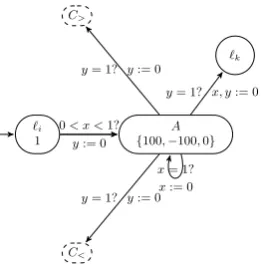
2 , reflecting the correct new counter values. y is reset on going to locationA. A time of one unit is spent at locationA. The value ofxis unchanged during this process due to the self loop onA. There are three possible rates that the environment can give to the scheduler, namely 100, -100 or 0 at locationA. The scheduler can go to any of the gadgetsC>, C<or to the location`k.
`i
1
A
{100,−100,0}
C>
C<
`k
0< x <1?
y:= 0
x= 1? x:= 0 y= 1? y:= 0
y= 1? y:= 0
[image:11.595.367.505.293.401.2]y= 1? x, y:= 0
Figure 4: Simulation of incrementc1 instruction
Assume that the time spent at `i is old2 +for some ≥0. In this case,x= old
2 +, y= 0 andz= 5−
old
2 +. The environment can force a check of the scheduler and catch his mistake, by choosing a rate of 100 at location A. This would makez= 105−old
2 +. If the scheduler wants to win, he must reach a mode in T, with the value of z inB∆(7). The best thing for the scheduler to do at this point is to chooseC>as his next location,
since it allows the value ofzto come back to 5−old
2 +. If the scheduler chooses to go toC<, he will be worse
off, making z even bigger, and if he chooses `k, the
environment can make sure that the scheduler never wins by choosing the rate 100 in all future gadgets.
Lets thus assume that the scheduler chooses to goto the gadgetC>in Figure 5. On entry, we havex=old2 +, y= 0 andz= 105−old
2 +. At locationO, the value ofxremains unchanged,ygrows to 1 and is reset, and z becomes z = 5− old
2 +. At location B, a time 1− old
2 −is spent, obtaining x= 0, y = 1−
old
2 − and z = 5− old
2 +−1(1−
old
2 −) = 4 + 2. If >0 and 2 >∆, then the scheduler has already lost, since adding 3 more toz at locationC does not help. Consider now the case that >0 and ∆−2=κ >0. At location D, a time of one unit is spent, and the environment can choose a rate as close to ∆ as he wants : in particular, he can choose a rate that is larger than κ, making the value ofz= 4+2+κ+ζ, for someζ >0. This means the scheduler can never reach a point in the ballB∆(7), even after adding 3 tozat locationC. If= 0, then irrespective of the rateκ∈(0,∆) chosen by the environment, the value ofz is 7 +κ ∈B∆(7), after adding 3 tozat locationC. Thus, if the scheduler made no mistake, he reaches a point inside the chosen ball.
O
−100
x= 1? x:= 0
B
−1
y= 1?
y:= 0
C 3
D (0,∆) T
0
x= 1? x:= 0
x= 1? x:= 0 x= 1?
[image:11.595.111.242.411.545.2]x:= 0
Figure 5: The gadget C>
Now consider the case when the scheduler spends an amount of time old
2 −, for some ≥ 0 at location li in Figure 4. Then we have x= old2 −, y = 0 and z= 5−old
2 −. At locationAin Figure 4, as seen above, the environment can assign any of the rates 100, -100 or 0 to the scheduler. If the environment wishes to catch the scheduler’s mistake, a rate of -100 will be assigned. The scheduler, if he chooses to goto C> or Go, will
surely lose, since the value ofz will decrease further, and will never reach a value inB∆(7); likewise, if the scheduler choosesGo, the environment can forever give a rate of -100. The best choice for scheduler is therefore, to pickC<. The gadgetC<is given in Figure 6.
On entry toC<, we have x= old2 −, y= 0 and z =
−95−old
2 −. At location O, the value ofxremains unchanged, y grows to 1 and is reset, andz becomes z = 4−old
2 −. At location B, a time 1−
old
2 +is spent, obtainingx= 0, y= 1−old
2 +andz= 5−old. A time old
2 −is spent at location C, obtainingz = 5−old+ 2(old
2 −) = 5−2.
Environment can then choose a rate−κ−ζ∈(−∆,0), for ζ >0. Thenz = 7−2−κ+ζ = 7−∆−ζ < 7−∆. This would result in scheduler losing. However, if = 0, then for any −κ∈(−∆,0), the value ofz is 7−κ∈B∆(7).
O 99 x= 1? x:= 0
B 1 y= 1?
y:= 0
C 2
D 2
E (−∆,0) T
0
x= 1? x:= 0
x= 1? x:= 0
x= 1? x:= 0 x= 1?
[image:12.595.371.505.53.162.2]x:= 0
Figure 6: The gadgetC<
The only remaining case is when the scheduler indeed picks the correct delay of old2 at location`iin Figure 4.
In this case, as seen above, the rates 100, -100 chosen by the environment does not affect the scheduler. In both these cases, scheduler has a winning strategy of choosing to go to one ofC<, C>and reach a value ofz
in the chosen ball. If= 0, and the environment picks the rate 0 at locationA, then the best strategy for the scheduler is to select`k, which marks the continuation
of the simulation of the two counter machine. As ex-pected, we will indeed have on entry intolk,x=y= 0
andz= 5−old
2 , marking the correct simulation of the incrementc1 instruction.
2. Simulation of a decrement instruction`i:c1:=c1−1; goto`k.
The construction of gadgets for the decrement instruc-tion is similar to that of the increment instrucinstruc-tion.
li
−1
2
A
{100,−100,0}
D>
D<
lk
0< x≤1?
y:= 0
x= 1? x:= 0 y= 1? y:= 0
y= 1? y:= 0
[image:12.595.109.242.119.224.2]y= 1? x, y:= 0
Figure 7: Simulation of decrementc1 instruction
The ideal amount of time to be spent by scheduler at `i is 2old. In this case,z = 5−2old, x = 2old, y = 0.
Assume that the time spent at`iis 2old+, for some >0. Then we havez= 5−2old−
2. At locationA, the environment picks one of the 3 rates 100, -100, 0. If he wants to force a check on the environment, he picks the rate 100, makingz= 105−2old−
2,x= 2old+, y= 0. As seen in the case of the increment gadget, the best strategy for the scheduler is to pick the gadgetD>.
O
−100
x= 1? x:= 0
B
−1
y= 1?
y:= 0
C 3 D
(0,∆) T
0
x= 1? x:= 0
x= 1? x:= 0 x= 1?
x:= 0
Figure 8: The gadget D>
Entry intoD>is made withz = 105−2old−2,x=
2old+, y= 0. One unit of time is spent atO, obtaining z = 5−2old−
2, x= 2old+, y = 0. At B a time 1−2old−is spent, obtainingz= 5−2old−
2−1(1− 2old−) = 4 +
2. A time of one unit is spent at C obtainingz = 7 + 2. Likewise, a time of one unit is spent atD, obtainingz= 7 +2+κ, whereκ∈(0,∆). If
2 >∆, then clearly, scheduler has already lost the game. If ∆−
2 >0, then κ ∈ (0,∆) can be chosen such thatκ >∆−
2 such that the value ofz /∈B∆(7). Note that if= 0, this is not possible, and scheduler can indeed reachz∈B∆(7).
Now consider the case when scheduler spends a time 2old−, for some >0 at`iin Figure 7. Then we have z = 5−2old+
2. Again, the environment can choose the rate -100 at location A, and the scheduler’s best strategy is to enter gadgetD<. Entry intoD<happens
withz=−95−2old+
2, x= 2old−, y= 0. One unit of time is spent atOobtainingz= 5−2old+
2, x= 2old−, y= 0. A time 1−2old+is spent at locationB obtainingz= 5−2old+
2−1(1−2old+) = 4−
2. One unit of time is spent atCobtainingz= 7−
2. Spending one unit at locationD with a rate−κ∈(−∆,0) gives z= 7−
2−κ. If
2 >∆, then the scheduler has already lost. If ∆−
2 >0, then the environment can always choose−κ∈(−∆,0) such thatz= 7−
2−κ <7−∆. Clearly, if = 0, this is not possible. and scheduler wins.
O 100 x= 1? x:= 0
B
−1
y= 1?
y:= 0
C 3
D (−∆,0) T
0
x= 1? x:= 0
x= 1? x:= 0
[image:12.595.60.296.269.587.2]x= 1? x:= 0
Figure 9: The gadget D<
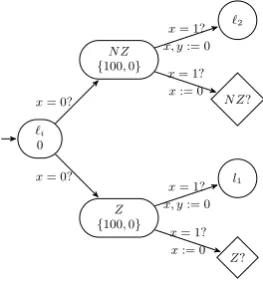
3. Zero Check Instruction. `i: ifc2= 0 goto`1 else goto `2.
Figure 10 describes the gadget for zero check of counter c2. No time is spent at location`i, and the scheduler
[image:12.595.373.506.503.607.2]with the simulation by choosing a rate 0, or could verify the correctness of scheduler’s guess by choosing a rate 100. One unit of time has to be spent at the location Z. Thus, if the scheduler decides to verify and chooses the rate 100, the value ofz will be 105−old. The en-vironment will check ifold= 21c1, for somec1 ≥0. If the environment chooses 100, the best strategy for the scheduler is to choose the gadgetZ?. Going to`1 does not help the scheduler to win, since the environment can pick the rate 100 in all future choice locations, en-suring that the scheduler cannot win.
`i
0
N Z
{100,0}
Z
{100,0}
`2
N Z?
l1
Z? x= 0?
x= 0?
x= 1?
x, y:= 0
x= 1? x:= 0
x= 1?
x, y:= 0
[image:13.595.336.541.50.237.2]x= 1? x:= 0
Figure 10: Zero Check
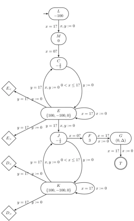
The gadgetZ? given in figure 11 is a check gadget which checks ifold = 2c11, for somec1 ≥0. The gadgetZ? is entered with z = 105−old,x= y= 0. A time of unit is spent at locationL, obtainingz = 5−oldand x, y = 0. If indeedc2 = 0, and if in addition, c1 = 0, then old = 1 and z = 4. In this case, the scheduler can go to the location F, spend a unit of time at F obtainingz = 7. This leads to the locationG, where the environment can pick any rate in (0,∆). One unit of time is spent inG, and in this case, we reach the mode T withz= 7 +κ∈B∆(7), forκ∈(0,∆). Clearly, the scheduler wins here since his guess aboutc2 being zero was correct.
In case old = 1
2c1 for c1 > 0, then from location M,
the scheduler cannot win by choosing location F as the next location, since the value of z on entry into G will be 8−old, where old = 1
2c1 for c1 > 0. If
8−old > 7 + ∆, then the scheduler has already lost. If 8−old≤7 + ∆, let 8−old= (7 + ∆)−p, for some p ≥ 0. Then p = ∆ +old−1 < ∆, since old ≤ 1
2. Thus, the environment can pick a rate p+ζ ∈(0,∆) such thatz= 8−old+p+ζ >7 + ∆.
Thus, if c1 > 0, the best strategy for scheduler is to goto locationC. The subgraph consisting of locations C, Dand gadgetsD<andD>simulates the decrement c1 instruction. The ideal time to be spent atCis 2old so that the value ofc1 is decremented by one. At loca-tionD, the environment can choose a rate 0 (in which case, scheduler will go back to location C) or a rate 100 (in which case scheduler will go to D>) or a rate
-100 (in which case, scheduler will go to D<). In the
case scheduler goes back to C, the new value of z is 5−2old, x=y= 0. The ideal time to be spent atCnow is 4old, and so on. At some point of time whenc1= 0,
L
−100
M 0
C
−1
2 F
3
G (0,∆)
T
D
{100,−100,0}
D<
D>
x= 1? x, y:= 0
x= 0?
x= 0? x= 0? x= 1?
x:= 0
x= 1? x:= 0
0< x≤1? y:= 0
y= 1? y:= 0
y= 1? y:= 0 x= 1? x:= 0 y= 1? x, y:= 0
Figure 11: The gadget Z?
we will obtainz = 4. At this point, the scheduler can take the transition toF fromC, and as seen above can reach T withz ∈ B∆(7). If the scheduler goes to F fromC when z = 5−oldfor some 0< old <1, then as seen above, on entry intoG, z = 8−old, and the environment has a choice of rate in (0,∆) such that scheduler loses.
The gadgetN Z? is given in Figure 12. This is entered into when the environment chooses a rate of 100 at locationN Z in Figure 10. The idea is to verify that indeedc2 is non-zero. Scheduler has to go through the locations C, E atleast once so that c2 is decremented atleast once (hence, c2 6= 0). The time elapse at C must be 3old, so that z = 5−old−2
3(3old) = 5− 3old, decrementingc2. The gadgetsE<andE>can be
designed similar to the gadgetsD<andD>to catch the
errors of the scheduler when the time elapse is 3old+ and 3old−, >0. The scheduler must visit theC, E loopc2 times (provided the environment gives rate 0 at location E everytime). When the rate 0 is given at locationE, scheduler can move to locationJ when c2 becomes 0. If c1 is zero, then we getz = 4 at the end of theC, E loop. Then fromJ, scheduler can go to locationF spending no time atJ, and reachT with z∈B∆(7). However, ifc1>0, then scheduler visits the J, Kloop untilc1= 0 (provided the environment gives a rate 0 at locationK). Whenc1= 0, the scheduler can move fromJtoF, and reach the target withz∈B∆(7). 4. The Halt location : The location labeledHalthas rate 1. The scheduler will reach here iff the two counter machine halts, and when the scheduler has simulated all the instructions correctly. The value ofzwill be 5−old, whereold=2c113c2, forc1, c2≥0. A non-deterministic amount of time can be spent by the scheduler here so thatzwill lie inB∆(7).
[image:13.595.110.242.181.323.2]L
−100
M 0
C
−2
3
F 3
G (0,∆)
T E
{100,−100,0}
J
−1
2
K
{100,−100,0}
D<
D>
E<
E>
x= 1? x, y:= 0
x= 0?
x= 0? x= 1?
x:= 0
x= 1? x:= 0 0< x≤1? y:= 0
y= 1? y:= 0
y= 1? y:= 0
x= 1? x:= 0
x= 1? x:= 0 y= 1? x, y:= 0
y= 1? x, y:= 0
0< x≤1? y:= 0 y= 1? x, y:= 0
y= 1? y:= 0
[image:14.595.66.280.190.542.2]y= 1? y:= 0