M
ethods
in
R
obust
and
A
daptive
C
ontrol
LIGE XIA
NOVEMBER 1988
A THESIS SUBMITTED FOR THE DEGREE OF
Doctor of philosophy
The doctoral studies were conducted with Professor John B. Moore, as supervisor,
and Professors Brian D.O. Anderson and Robert R. Bitmead, as advisors.
" I hereby declare that the results presented in this thesis, except as otherwise
explicitly stated, are the results of original research and have not been submitted for
any other degree to any other university or educational institution."
Canberra, November 1988
LigeXIA 7
Department of Systems Engineering
Research School of Physical Sciences
The Australian National University
GPO Box 4 ACT 2601
ACKNOWLEDGMENT
It has been one of my most pleasant time periods when I undertook my doctoral
studies in the department of systems engineering. Firstly, I would like to thank my
supervisor, Professor John B. Moore, not only for his guidance, encouragement,
criticism and supervision in academic, but also for his kind and selfless help on
personal matters. I believe that the teacher-student relationship means much more
than the words themselves say, and it will be treasured.
Many thanks also go to Dr. Lei Guo and Professors B.D.O. Anderson, R.R.
Bitmead, and M. Gevers for their kind advice and helpful discussions from time to
time. The staff and students of the department of systems engineering deserve the
acknowledgment for providing the high stimulating and fruitful environment. And
the financial support from the Australian National University is appreciated.
It is very hard to express my appreciation for the support from my dear wife
ABSTRACT
The thesis develops control system design methods and theory with an emphasis on
achieving robust off-line and on-line controller designs. The topics studied cover
four problem areas.
In the first problem area the objective is to improve controller loop robustness of an
initial design. The first contribution we make here is the convenient parametrization
of the class of model matching controllers, this being the first step to apply standard
H^-optimization techniques to improve robustness. The second contribution in this
topic is to extend the techniques of loop transfer recovery in linear quadratic
Gaussian (LQG) designs to cope with nonminimum phase plants.
In the second problem area, the objective is to develop central tendency adaptive
control methods so as to improve the transient performance of those standard
adaptive schemes by taking the uncertainty of the plant parameter estimates into
account in constructing the adaptive controller. Our contributions here are to the
development of central tendency adaptive pole assignment and central tendency
adaptive LQG control.
The third problem we tackle is avoidance of ill-conditioning which arises with the
estimation and control of overparametrized systems. Here algorithms are proposed
to cope with overparametrization in the signal model and achieve convergence to the
unique model estimate which corresponds to the non-overparametrized model.
Based on these estimation algorithms, a central tendency adaptive pole assignment
ABSTRACT
which are possibly overparametrized. Furthermore, an identification scheme is
proposed based on Kalman filter ideas to deal with possibly overparametrized
systems with model order and plant parameter changes.
For the last problem area, motivated by the third problem area applications, we give
some analysis results on standard estimation algorithms. One is to show that for
identification of multidimensional linear regression models, the strictly positive real
(SPR) conditions imposed on the plant noise can be side-stepped by introducing
artificial noise into the regression vector to make the combined noise whiter.
Convergence results are achieved without the SPR condition satisfied, and it is also
shown that the whiter the noise environment, the more robust are the algorithms.
Another result is to show how to side-step the strictly positive real condition in
general ARMAX model identifications. This is achieved by a unique
overparametrization so that the strictly positive real conditions can be relaxed at
arbitrary degree. The last one is about tracking unknown randomly changed plant
parameters, for linear stochastic system identification a using standard Kalman filter
algorithm. Here we develop asymptotic properties of the algorithm and establish the
PREFACE
The material included in this thesis is the results of original research co-operatively
working with Prof. Moore (my supervisor) and /or Dr. Guo. The contributions on
the joint research work with which I feel most closely identified with are the papers
with myself as first author. More specifics of my contributions are now
summarized.
As a first year graduate student, my contributions to the topics "Central tendency
adaptive pole assignment" and "Loop recovery and robust state estimate feedback
design" were to developing some of the technical results and to the simulation
studies to demonstrate the effectiveness of the results. For the project "On
improving control loop robustness of model matching controllers", some of my
own insights and technical contributions were critical to the successful formulation
and derivation of the results. The work on "Adaptive LQG controllers with central
tendency properties" is primarily my own work, building on the ideas of the central
tendency adaptive pole assignment study.
For the project "On adaptive estimation and pole assignment of overparametrized
systems" the key theorems and proofs were developed in the first instance by
myself with feedback from Prof. Gevers. Later these were enhanced to the
stochastic case by working jointly with my supervisor. For the papers "Recursive
identification of overparametrized systems" and "Adaptive estimation in the
presence of order and parameter changes", I was able to work more independently.
models”, my contributions were to initially quantify the level of injected white noise
to side-stepping the positive real condition on noise color, and to provide the
insights crucial to a number of lemmas in the paper. In the paper 'Tracking
randomly varying parameters”, I contributed to the development of some of the
theorem proofs. In the paper "Computation of H°°-norms of polynomials", a special
case study in details turns out to be very helpful for the algorithm development. For
the paper "Identification / prediction algorithms for ARMAX models with relaxed
positive real conditions", I involved the development of almost all the theorem
Co n t e n t Ta b l e
Chapter 1. Introduction
Part 1. On Improving Controller Robustness
Chapter 2 Loop Recovery and Robust State Estimate Feedback Designs
§ L Introduction
§ 2. Loop recovery
§ 3. A design approach - illustrative example
§ 4. Frequency shaped estimation
§ 5. Conclusions
Chapter 3 On Improving Control - Loop Robustness of
Model - Matching Controllers
§ 1. Introduction
§ 2. The class of stabilizing controllers
§ 3. A class of model matching controllers
§ 4. Improving robustness via H°°-optimization
§ 5. Conclusion remarks
Chapter 4 Computation of H°°-norms of Polynomials
§ 1. Introduction
§ 2. Algorithm description and main results
§ 3. Convergence analysis
§ 4. Example studies
CONTENT TABLE
Part 2. Central Tendency Adaptive Control
Chapter 5 Central Tendency Adaptive Pole Assignment
§ 1. Introduction
§ 2. Central tendency adaptive pole assignment
§ 3. Least squares convergence
§ 4. Simulation results
§ 5. Conclusions
Chapter 6 Adaptive LQG Controllers with Central Tendency Properties
§ 1. Introduction
§ 2. Adaptive LQG controllers via Riccati recursions
§ 3. Central tendency adaptive LQG control
§ 4. Conclusions
Part 3. Adaptive Schemes for Overparametrized Systems
Chapter 7 Adaptive Estimation and Pole Assignment of
Overparametrized Systems
§ 1. Introduction
§ 2. Algorithms and results - white noise case
§ 3. Adaptive pole assignment
§ 4. A property of Sylvester matrices
§ 5. Simulations
§ 6. Conclusions
CONTENT TABLE
Chapter 8 Recursive Identification of Overparametrized Systems
§ 1. Introduction
§ 2. Algorithm
§ 3. Convergence
§ 4. Simulations
§ 5. Conclusion
§§ Appendix
Chapter 9 Adaptive Estimation in the Presence of
Order and Parameter Changes
§ 1. Introduction
§ 2. Perturbed Kalman filter detection / identification scheme
§ 3. Simulations
§ 4. Conclusions
Part 4. Some Analysis Results on Estimation Algorithms
Chapter 10 Robust Recursive Identification of
Multidimensional Linear Regression Models
§ 1. Introduction
§ 2. Algorithm description and main results
§ 3. Preliminary theory
§ 4. Proof of theorems
§ 5. Conclusions
CONTENT TABLE
Chapter 11 Identification /Prediction Algorithms for ARMAX Models
with Relaxed Positive Real Conditions
§ 1. Introduction and background
§ 2. Transformed ELS algorithms and theorems
§ 3. D-step-ahead prediction
§ 4. Extension to multivariable ARMAX models
§ 5. Example studies
§ 6. Conclusions
Chapter 12 Tracking Randomly Varying Parameters
§ 1. Introduction
§ 2. Tracking error bound
§ 3. Conclusions
§§ Appendix
Ch a p t e r l INTRODUCTION
When one wants to control a plant, a starting point is the a priori knowledge about
the plant and any assumptions concerning the plant The resulting control scheme is
very much dependent on such assumptions and a priori knowledge of the plant, as
well as the control objectives. Certainly, with different assumptions, the control
strategy varies, and the problems and difficulties in designing the controllers differ
accordingly.
If one assumes that the plant is known exactly and is precisely described by a linear
dynamical stochastic signal model which prescribes the variation with respect to
time, the system order and the plant parameters, then a stabilizing fixed (non-
adaptive) controller can be designed using text book methods. However, the true
plant dynamics, as is inevitable in practice, may not perfectly match the assumed
signal model. It is known that such a mismatch between the signal model and actual
plant, may cause serious problems, namely cause instability of the closed loop
system consisting of the actual plant and the controller designed for the nominal
plant. This motivates for us the concept of a robust controller design. A robust
controller is one which can cope with some mismatching between the signal model
and the plant, achieving suitable stability margins when applied to the nominal
plant. The robustness can be with respect to unmodelled dynamics, or to plant
parameter estimation errors, or to both. Improving control loop robustness
properties of a nominal design has attracted much attention, and there are many
approaches proposed to do this. Loop transfer recovery, and H°°-optimization are
CH 1 INTRODUCTION
In many situations, the plant dynamics are only assumed to be known as one
member of a specified class of models (say a linear system with known order but
unknown parameters). Or they may drift very slowly inside of this class of models.
To cope with such situations, the concept of adaptive control is relevant Adaptive
control normally consists of two steps, at least in what is known as indirect
adaptive control. First, the plant parameters are estimated, then the controller is
designed based on the information gained from the estimation of the plant. Thus the
"learning" of the plant and the "controlling" of the plant take place in parallel, and as
time goes on, it is the intention that as the plant parameters are identified, then the
controller converges to the one which would have been used if the plant parameters
were known. In the course of such adaption, the way to balance the effects of
"learning" and "controlling" makes the complexity of the adaptive control schemes
differ considerably. There are two extremes. One is called certainty equivalence
principle, and the other is called dual control. In the certainty equivalence principle,
the adaptive controller is designed using the estimates of the plant as if they were
the true plant. This approach is easy to implement and simple to use as an on-line
scheme. However, its disadvantage is that it can only be optimal asymptotically and
the transient performance may be unnecessarily poor, even intolerable. On the other
hand, the dual control objective is to give a "best" control in the presence of plant
uncertainties. However schemes proposed under this heading are very formidable
to design and are almost impossible to be implemented on-line. Thus to design an
adaptive scheme which has a reasonable transient performance and also is easy to
implement becomes a challenging task with the promise of a high payoff.
It is common, in many adaptive schemes, to assume that the plant to be controlled
CH 1 INTRODUCTION
However, the choice of the signal model order, in some situation, is not an easy
job. If the order is selected too low (it is called underparametrization), then the
unmodelled dynamics can be destabilizing the whole system, this suggests that
there is a tendency in practice to overparametrize the signal model to be on the
"safe" side, that is to choose the order higher than it is. However, when an adaptive
estimation algorithm (say least squares or Kalman filter) is employed to identify an
overparametrized system, there is inevitably a lack of excitation in the regression
vectors and normally there is no guaranteed convergence in this situation. In
general, near pole zero cancellations in the estimated plant are expected, and they
can be located anywhere being sensitively dependent on the initial conditions and
noise sampling path. Furthermore, based on those estimates of the plant, some
adaptive control schemes (typically pole assignment control) could ineluctably lead
to excessive control signals (or so called ill-conditioned). Therefore the
overparametrization on the signal model emerges as a significant problem.
In this thesis, we present our solutions to such robust and adaptive control
problems as mentioned above. The solutions are only solutions under certain
assumptions, and so are not claimed to be complete in any way. However, we
believe they are an advance on current methods in the literature. The thesis consists
of four parts based on the research papers published or submitted for publication in
journals and international conferences, and is organized as follows.
In Part I, we develop and generalize some techniques for improving the controller
loop robustness properties of an initial design. It is known that when a controller is
designed for a nominal plant to satisfy some performance requirement, and achieves
CH 1 INTRODUCTION
robust controller in the sense of tolerating plant changes form the nominal plant, or
in other words the uncertainty of the plant parameters. Some approaches have been
proposed to improve controller loop robustness while keeping the closed loop
transfer function unchanged. One of the approaches is called "loop transfer
recovery” (LTR) which mainly focuses on the linear quadratic Guassian (LQG)
control design, but can be applied to any state estimate feedback based design. The
idea of LTR is to represent the plant uncertainty by adding fictitious noise to the
plant input while designing the LQG controller. For minimum phase plants, as the
magnitude of the fictitious noise increases the control loop transfer functions
approach to those for the state feedback design, which have attractive robustness
properties. Then we say "loop recovery" occurs. Here as Chapter 2, we present our
generalization on LTR, namely to handle non-minimum phase plant, which is based
on the published paper [pi]. In Chapter 2, the loop recovery technique has been
generalized for nonminimum phase plants in the following sense. The open loop
properties of certain partial state feedback designs are recovered in a state estimation
feedback controller design involving the addition of fictitious plant noise. The
partial state is the state of a minimum phase factor in a minimum phase, all-pass
factored form model. Of course, robust designs are expected only when these are
achieved for the case of partial state feedback of only the minimum phase factor
states. This may not always be possible. For the case on minimum phase plants,
known designs and theory are recovered as a special case. The theory and designs
of this chapter generalize to include frequency shaping of both the control objectives
and the loop recovery.
Another approach of improving control loop robustness properties of an initial
CH 1 INTRODUCTION
most robust controllers among those which satisfy the performance requirement
(say achieve a specific closed loop transfer function) or so called "model matching
controller". Here in Chapter 3, we present the results on parametrization of the class
of all model matching controllers, and a procedure to search for the most robust
one, by performing an H°° optimization. These are based on the published paper
[p2]. In this chapter, the class of all stabilizing controllers, for a two-degree-of-
freedom control system which achieve a prescribed achievable transfer function, is
first characterized. The characterization is in terms of an arbitrary proper stable
transfer function. With this characterization, robust model matching is formulated
as a standard H°°-optimization problem. This means that standard controller designs
for a nominal plant, such as LQG ones, can be enhanced to give improved
robustness properties using H°°-design techniques.
It is observed that in practice, to calculate the value of the H°° norm is usually done
by a rather trivial method, i.e. plotting the absolute value of the function concerned
on the unit circle. This involves some ad hoc selection of plotting intervals and
interpolation to achieve an appropriate accuracy. Here in Chapter 4, we propose a
recursive algorithm for the computation of H°° norm of polynomials or finite
impulse response (FIR) transfer functions based on the published paper [p3]. The
algorithm is shown to converge monotonically and the convergence rate is also
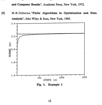
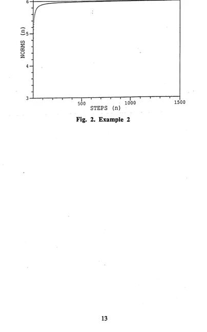
established. Some examples are presented to illustrate the algorithm.
We report, in Part II, applications of so called central tendency control concept to
adaptive pole assignment control and LQG control. As mentioned above, in
designing indirect adaptive controls, there is a range of schemes to choose between
CH 1 INTRODUCTION
When an adaptive scheme based on the certainty equivalence principle is employed,
it can only be optimal asymptotically and there will be in general, circumstances
where the transient performance is unnecessarily poor. And dual control normally is
too formidable to be a practice proposition for on line schemes. In order to avoid
excessive control signals due to inaccurate estimates of the plant during transient,
and to achieve an on-line implementable scheme, the central tendency control was
proposed. In the central tendency control, adaptive controllers are designed using
measures of central tendency of the a posteriori probability function of the controller
parameters. That is, given knowledge of plant uncertainty at each time instant, from
estimation algorithms, and a controller design rule, the controller parameters is
sought which maximized the likelihood of achieving the control objectives. Here we
report the results on central tendency adaptive pole assignment control and LQG
control respectively as Chapter 5, and Chapter 6 based on the papers [p4], [p5]
presented in international conferences.
In Chapter 5, the concept of central tendency adaptive control is applied to adaptive
pole assignment. At any iteration, given plant parameter estimates and their
uncertainty, a controller is designed which is "most" likely to achieve the pole
assignment objectives. Simulations show a factor of 100 improvement, in transient
response in one example, over certainty equivalent adaptive pole assignment
schemes at least for one example.
In Chapter 6, it is first observed that one particular standard certainty equivalence
based version of an adaptive LQG controller in the literature tends to have a better
transient performance than others of comparable complexity. Why is this so? Can
CH 1 INTRODUCTION
schemes be modified to have improved transient performance? The main result of
this chapter makes clear that improved transient performance tends to occur when
the design rule is linearized so that the controller parameters are the most likely
ones, according to the control design rule, given the plant uncertainty. In addition,
since there is an option of different linearized design rules at each iteration, a
particular one can be chosen to maximize a central tendency measure, thereby
achieving central tendency adaptive LQG control. For central tendency adaptive
LQG schemes, there is avoidance of excessive control action due to ill-conditioning
associated with near unstable pole zero cancellation in plant estimates.
Part m is devoted to tackling the problems of overparametrization in adaptive
schemes. For adaptive estimation / control scheme design, as mentioned early, it is
common to assume a linear input -output signal model of specified order with
unknown parameters. Since the underparametrization may cause destabilizing, there
is a tendency in practice to overparametrize the signal model to be on the "safe"
side. Thus overparametrization emerges as a significant problem in some
applications. A specific situation is when the presence of some deterministic
disturbances such as bias is assumed, when in fact any such disturbances are
negligible. With overparametrization, there is a danger of ill-conditioning in
adaptive estimation and in some adaptive control. When an adaptive estimation
algorithm (say least squares, or Kalman filter) is employed to identify an
overparametrized system, there is inevitably a lack of excitation in the regression
vectors and normally there is no guaranteed convergence. Also insufficient
excitation can lead to estimation with near pole-zero cancellations in the complex z-
plane. Such pole-zero cancellation can occur anywhere sensitively dependent on the
CH 1 INTRODUCTION
adaptive control schemes, such as pole assignment scheme. We propose an
approach based on standard identification algorithms (namely least squares and
extended least squares) to cope with adaptive estimation of overparametrized
systems. The key idea in this approach is to introduce excitation signal into the
regression vectors so as to enforce artificially the regression vector to have suitably
excitation, even when the systems are overparametrized.
Here, as Chapter 7, our published paper [p6] is included. In this chapter, a first
step is taken to avoid ill-conditioning in adaptive estimation and pole assignment
schemes for the case when there is a signal model overparametrization. The
methods proposed in this chapter are relatively simple compared with on-line order
determination, being based on introducing suitable excitation in the "regression"
vector of the parameter estimation algorithms to ensure parameter convergence. For
the case when the model are non-unique in that pole zero cancellations can occur,
the algorithms seek to estimate the unique model where the cancellations occur at
the origin. Applying estimates of this (unique) model turns out to avoid ill-
conditioning in central tendency adaptive pole assignment For the case of one pole
zero cancellation the convergence theory of the algorithm is complete.
Following on from our initial work, we present generalized results as Chapter 8
based on the published paper [p7]. In this chapter, a recursive identification
algorithm based on extended least squares is proposed to deal with the contingency
of overparametrization. The algorithm proposed here is relatively simple compared
to those involving on-line order determination, being based on adaptively
introducing suitable excitation into the algorithm to avoid ill-conditioning. In the
CH 1 INTRODUCTION
appropriately stochastically perturbed. The algorithm is shown to converge to a
unique defined signal model with any pole zero cancellations at the origin. Ill-
conditioning is avoided.
In Chapter 9, based on the paper [p8], we report further research on tracking
parameters changes in the presence of order changes. An approach to adaptive
estimation and control is given when there are jump parameter changes which
include order changes. Order changes can be viewed as the introduction of
overparametrization, which in conventional algorithm causes ill-conditioning. Here,
modified algorithms which involve the introduction of noise into the calculations are
proposed and studied by theory and simulations.
Part IV consists of Chapters 10, 11 and 12, reporting some analysis results on
adaptive estimation algorithms. One of them deals with linear regression model
[p9]. It is known that stochastic adaptive estimation and control algorithms
involving recursive prediction estimates have guaranteed convergence rates when
the noise is not ’’too" colored, as when a positive real condition on the noise model
*
is satisfied. Moreover, the whiter the noise environment the more robust are the
algorithms. Chapter 10, which is based on the published paper [p9], shows that for
linear regression signal models the suitable introduction of white noise into the
estimation algorithm can make it more robust without compromising on
convergence rates. Indeed, there is guaranteed attractive convergence rates
independent of the process noise color. No positive real condition is imposed on the
noise model.
However, the techniques used in Chapter 10 do not appliable to a general ARMAX
CH 1 INTRODUCTION
extended least squares algorithms are proposed for ARMAX model identification
with the objective of avoiding the positive real condition associated with standard
equation error and output error algorithms. This is achieved by an
overparametrization at the cost of additional richness requirements on excitation
signals, but without introducing ill-conditioning or infinite dimensional calculations
as in earlier methods. Results for the case of D-step-ahead prediction ELS
algorithms for ARMAX models also explored in this chapter and some simulation
studies are included to assess the relative performance characteristics of the
proposed algorithms.
The other analysis result is [pi 1] on the standard algorithm namely Kalman filter. It
is known that in linear stochastic system identification, when the unknown
parameters are randomly time varying and can be represented by a Markov model, a
natural estimation algorithm to use is the Kalman filter. In seeking an understanding
of the properties of this algorithm, existing Kalman filter theory yields useful
results only for the case where the noises are Guassian with covariances precisely
known. In other cases, the stochastic and unbounded nature of the regression
vector (which is regarded as the output gain matrix in state space terminology)
precludes application of standard theory. In Chapter 12, based on the paper [pi 1],
we develop asymptotic properties of the algorithm, in particular, we establish the
tracking error bounds for the unknown randomly varying parameters. ¥
A summary is drawn in Chapter 13 as the conclusions for the thesis and also some
CH 1 INTRODUCTION
Pu b l i c a t i o n s
[pi] J.B. Moore and L. Xia, ’’Loop Recovery and Robust State Estimate
Feedback Designs", IEEE Transaction on Automatic Control
Vol.AC-32, pp. 512-517, 1987. Also see Proc. of ACC, pp. 1807- 1812, Seattle 1985.
[p2] J.B. Moore, L. Xia and K. Glover, "On Improving Control-Loop
Robustness of Model-Matching Controllers", Systems and Control Letters Vol. 7, pp. 83-87, 1986.
[p3] L. Guo, L. Xia and Y. Liu, "Recursive Algorithm for the Computation of
H°°-Norm of-‘Polynomials", IEEE Transaction on Automatic Control Vol.AC-33, Oct. (to appear) 1988.
[p4] J.B. Moore, T. Ryall and L. Xia, "Central Tendency Adaptive Pole
Assignment", IEEE Transaction on Automatic Control Vol.AC-34, Jan. (to appear) 1989. Also see "Central Tendency Pole Assignment",
Proc. of 25th CDC, pp. 100-105, Athens, Greece. 1986.
[p5] L. Xia and J.B. Moore, "Adaptive LQG Controllers with Central
Tendency Properties", to appear in Proc. of IF AC Symposium on Identification and System Parameter Estimation, Beijing, 1988.
[p6] L. Xia, J.B. Moore and M. Gevers, "On Adaptive Estimation and Pole
Assignment of Overparametrized Systems", Int. J. of Adaptive
Control and Signal Processing, Vol. 1 pp. 143-160. 1987. Also see
CH 1 INTRODUCTION
[p7] L. Xia and J.B. Moore, "Recursive Identification of Overparametrized
Systems", IEEE Transaction on Automatic Control Vol. AC-33,
Dec (to appear), 1988.
[p8] L. Xia, V. Krishnaumrthy and J.B. Moore, "Adaptive Estimation in the
Presence of Order and Parameter Changes", submitted to Int. J. of Adaptive Control and Signal Processing.
[p9] L. Guo, L. Xia and J.B. Moore, "Robust Recursive Identification of
Multidimensional Linear Regression Models", Int. J. Control, (to appear), 1988. Also see Proc. of IFAC Workshop on Robust Adaptive Control. 1988.
[10] J.B. Moore, M. Niedzwiecki and L. Xia, "Identification / Prediction
Algorithms for ARMAX Models with Relaxed Positive Real Conditions",
submitted to Int. J. of Adaptive Control and Signal Processing.
[pi 1] L. Guo, L. Xia and J.B. Moore, "Tracking Randomly Varying
PART I
C h a p t e r 2
LOOP RECOVERY AND ROBUST STATE ESTIMATE
FEEDBACK DESIGNS
1. Introduction
It is well known that plant input robustness properties of a state feedback (SF)
design, such as measured by phase margins for example, can evaporate with a state
estimate feedback (SEF) design [l]-[5]. An important class of SF design is linear
quadratic (LQ) design, with the associated SEF design being then linear quadratic
Gaussian (LQG) design.
A technique to improve robustness of SEF based designs, such as LQG designs, is
to represent the plant uncertainty in the frequency band of interest by the addition to
the plant input of fictitious noise in this band, [5,][6]. Such a technique for
minimum phase plants leads to "loop recovery", because as the magnitude of the
fictitious noise increases, the open loop transfer functions, and thus loop
robustness properties, approach those for the SF design. The recovery of the SF
robustness properties in the frequency band of the noise is at the expense of a
reduced performance in the frequency band of the noise. The theory for the case of
fictitious white noise is developed in [5], while the case of added colored noise is
studied in [6].
In this chapter, the notion of loop recovery is extended to certain classes of SEF
designs for nonminimum phase plants. The results are developed using an all-pass
/ minimum phase (i.e. inner/outer) factored form for the plants. The SEF controller
CH 2 LOOP RECOVERY
initial state feedback design must constrain the feedback to feedback of only the
minimum phase factor states, giving an outer state feedback (OSF) design (possibly
dynamic). The addition of fictitious noise at the input to the minimum phase factor
ensures that when state estimators are employed, there is loop recovery. Of course,
certain nonminimum phase plants can never be "robustly" controlled, nor
"robustly" controlled using state feedback of only the minimum phase factor states.
In the latter case, when loop recovery is applied, it is not expected that the resulting
design will be "robust".
In the case of two degree of freedom design, the technique of [8] building on those
of [3] can be applied. A particularly convenient formulation arises using the results
of [9].
In Section 2, a class of controllers is defined for which loop recovery properties are
guaranteed. A design approach and an example design are included in Section 3 to
add insight. Section 4 summarizes new results for frequency shaped state
estimators by dualizing control results in [10]. Such results are useful for frequency
shaped loop recovery. Conclusions are drawn in Section 5.
2. Loop Recovery
In this section, we consider in turn factored signal models, state estimation and
controller constraints for loop recovery.
Factored Form Plant Model:
CH 2 LOOP RECOVERY
function matrix W(s). Consider also a standard inner/outer factorization of W(s)
as, see [11]
Here W^s) is asymptotically stable, and "inner", or equivalently "all-pass", in that
Wi(-s)xWi(s) = I. Also, W°(s) is "outer" or "minimum phase" in that W°(s) has full
rank for s in the right-half plane Re[s] > 0. Here also, W^s) has its poles in Re[s] <
0, and the zeros of W°(s) are in Re[s] < 0. Should W(s) be minimum phase, then
trivially W^S) = I, W°(s) = W(s). Unstable modes of W(s) appear in W°(s). As
guaranteed in the state space factorization approach of [11], there may exist
cancellation of the poles Wi(s) and the left half plane zeros of W°(s), and none
between the zeros of Wi(s) and the poles of W°(s). Actually, imaginary axis zeros
of W(s) are not permitted for the algorithms of [11], but are permitted in much of
the subsequent theory.
W(s) = W°(s)Wi(s) (2.1)
* W(s) = c ’VsI - aV bP
(a) Deterministic Model
(b) Factored (nonminimal) Model
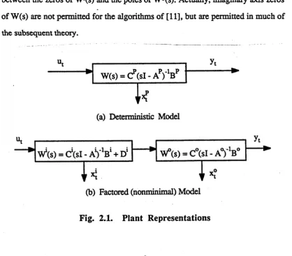
[image:27.523.49.468.380.747.2]CH 2 LOOP RECOVERY
R eferring to Figure 2 .L a, let us consider a m inim al state space realization
{AP,BP,CP } for the plant with transfer function W (s) = Cp(sI-A p)_1B p and state
xpt. Referring to Figure 2 .l.b , let us consider a non-m inim al representation o f the
plant factored into its all-pass and minim um phase factors. The all-pass system,
{A*,B*,C*,D*} assum ed m inim al, has states x \ and a transfer function W ^s) =
[C10 1(s)Bi+Di] where 3>i(s) denotes (sI-A1) ' 1. Also D 1^ 1 = I. The minimum phase
system {A °,B0,C°}, assumed minimal, has states x°t and a transfer function W °(s)
= C°O0(s)B°, <D°(s) = (sI-A0)-1.
Stochastic Model:
Consider the factored form m odel o f Figure 2. L b, but with process noise v tp =
N [0, Q p] and m easurem ent noise wt = N [0,R p ]. These are assum ed to be
independent, zero mean and white, having covariance m atrices Qp > 0, Rp > 0
respectively. For simplicity, the process noise is assum ed to be added at the plant
input and Qp is taken as Qp = qpI. In addition there is included in the m odel a
fictitious process noise vft, assum ed to be inserted at the input to the m inim um
phase factor. Its purpose is to achieve loop recovery properties in its frequency
band, It can be view ed as representing the effects o f plant uncertainty in this
frequency band. In the first instance, let us consider the case o f white fictitious
noise vft = N[0,ql]. Denoting the state o f the factored form plant m odel as xt, then
its state space equations are
vt = [ y p j . Axt + But + Tvt, y t = Cxt + w t
CH 2 LOOP RECOVERY
Should W(s) be minimum phase, then x t = xpt = x °t, otherwise, x t is a
non-minimal state vector.
State Estimator
Applying Kalman filter theory [1],[2] to the stochastic (non-minimal) plant model
(2.2) yields the time invariant estimator
Axt + But + K(yt - Cxt), x0 = 0, K = PC^R-1,
PA"1 + AP - PO R -'C P + Q = 0, P > 0 (2.3)
It is easy to verify that for QP = qPl the partitioned solution P has block P12 = P2lx
= 0. Also Ki = 0 (details to be seen in Lemma 1). Then for zero initial conditions,
(2.3) gives
x(s) = (si - A + KC)'l[Bu(s) + Ky(s)], or x*(s) = O i(s)Biu ( s ) ,
£°(s) = <50(s) {K0[y(s)-C°x°(s)] + B°W '(s)u(s)), (2.4)
The estimation (2.3) is well defined when [A,C] is detectable, and in addition is
i
asymptotically stable when [A,(JJ is stabilizable. Since the all-pass factor here is
asym ptotically stable, these conditions sim plify as [A °,C °] detectable,
_i_
[A°,B°(qI+qpDiDix)2] stabilizable. These are trivially satisfied for all finite q > 0,
CH 2 LOOP RECOVERY
Frequency Shaped Estimation:
For practical control law design using loop recovery techniques applied to minimum
phase plants [6], the fictitious noise is usually frequency shaped so that robustness
is achieved in the frequency band where otherwise the design is not robust. Thus
fictitious noise is usually injected only at frequencies in the vicinity of the cross
over (loop unity gain) point. The controller and performance is then unchanged
outside such frequency bands. For practical designs, in the more general setting of
nonminimum phase plants as here, the same thinking applies.
Frequency Shaped Fictitious Noise: Assume that the frequency shaped
fictitious noise vft has a power spectrum qQf(s) = qQfx(-s) which is
nonsingular a.e. The minimum phase stable spectral factor of Qf(s) is denoted
by[Qf(s)F. (2.5)
Frequency shaped estimation theory, see Section 4, now applies. Leaving aside any
frequency shaped estimation of since this is not required in subsequent loop
recovery theory, the state estimation (2.4) generalizes as,
x°(s) = <D°(s) {K°[y(s)-C°x°(s)] + B°W'(s)u(s)}, (2.6)
where K°(s) is given from the spectral factorization
C°O0(s)Q0(s)O°(-s)TC0T+R = F°(s)RF°(-s)x
C°a>o(s)K°(s) = [F°(s) - 1], (2.7)
Here Q°(s) is the spectrum of the noise signals affecting the states x°t and consists
CH 2 LOOP RECOVERY
prefiltered by B°Wi(s). We assume that there are no pole-zero cancellations in
C°d>0(s)Q0(s)O°(-s)TC0X. Here also, F°(s) is the unique minimum phase spectral
factor with the same poles as <E>°(s) and the stable poles of Q°(s). The theory of
Section 4 tells us that with A0, C° observable, a stable proper K°(s) can be
constructed satisfying (2.7) so that the optimal estimation (2.6) can be
implemented. Indeed this property can also be verified using state space models for
the shaping filter and augmenting those to the plant model and applying standard
Riccati theory and spectral factorization concepts.
OSF Controller
Consider the stabilizing outer state feedback control law, ignoring initial conditions,
and associated open loop transfer function as
uOSF(s) = lOSF(s)xo(s), W 8£F(S) = LOSF(s)<i>o(s)BoW'(s) (2.8)
For the main result of this section, there is no concern about how LOSp(s) is
designed. However, to use the result as a design tool we present subsequently one
approach to the design of L0SF(s) based on LQ/H°° methods.
SEF Controller:
From (2.8), we see that the outer state feedback control u0SF consists of dynamic
feedback of the outer states x°t . The corresponding state estimate feedback
controller using the estimator (2.3) to achieve estimates x°t, replaces x°t with x°t .
Thus in obvious operator notation,
CH 2 LOOP RECOVERY
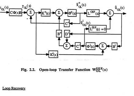
O f course, ignoring initial conditions, uOSF(s) = uSEF(s^ However, the open loop
transfer functions W § £ F(s), W ^ £ F(s) differ. The transfer function w £ £ F(s) is
depicted in Figure 2.2 and is (with K> = 0, LISF = 0)
W §£F(s)={TLOSF(s) p +o o ( s)Ko c o]-l<D0(s)B0 }-10 0(s)B0W (s) (2.10)
u^s)___ ya.(s)
--- Hca<sy|-»»(s)--*|K
0
(s)[-»(s
A w , \
XCL(S>
C c
L®F(s
*OL(S)
uo6^
b£
Lisf(s) =0
0 '(s )
K‘(s)
h©H
B1Fig. 2.2. Open-loop Transfer Function W ^ F(s)
Loop Recovery
Loop recovery at the plant input is said to occur when for alm ost all s, the open
loop state estim ate feedback transfer function approaches the open loop state
feedback transfer function as adjustm ents are made to the design o f the state
estim ator. H ere the adjustm ent is that q —» °o and we seek the loop recovery
property
[image:32.523.45.485.238.554.2]CH 2 LOOP RECOVERY
Lemma 1: Consider the factored plant (2.2) state estimator (2.3) and
feedback control laws as in (2.9). Then for the case when QP = qPl
P12 = P21t = 0, K> = 0, Ko = PnC ^ R -1, (2.12a)
P11 A ^h-A°P11-P11O ^ R '1 C°Pii+(qp+q)B°B01 = 0, P n > 0 (2.12b)
Proof: The solution P > 0 of (2.3) is known to be unique under minimality of
[A°,B°,C°] as in early discussions. We first show that taking P12 = P21X = 0 leads
to a solution P > 0 to conclude that indeed P12 = P2ix = 0. Taking Pi2=P21x = 0 in
(2.3) gives
P22Aix + AiP22 + qPEPBi* = 0, P22 ^ 0
which has a unique solution with [A^B*] stabilizable as here. From [12] Theorem
5.1, with a mild extension to include the non-square case we have
Ö P22 + qPDiß* = 0
Now (2.3) yields (2.12b) which has a solution with [A°,B°,C°] minimal as here.
Consequently, P = Diag[Pn P22] ^ 0 is a solution to (2.3). Thus P12 = P21x = 0.
Then (2.12) holds. AAA
Remark The important aspect of this lemma is that the estimator gain is
constructed in terms of only the outer factor parameters A°,B°,C° and the
covariances R, qPl, ql. For the frequency shaped fictitious noise as in (2.5), the
same results hold as established using the results of Section 4. Again Ki = 0 and
CH 2 LOOP RECOVERY
Theorem 1 Consider the plant in factored form (2.1), (2.2) with
[A°,B°,C0] minimal, and the optimal state estimation (2.6) under (2.5),(2.7).
Consider also the SEF controller, as above, based on the OSF feedback
control law (2.8). Then
Lim^ c°o°(s)[I + K°(s)C°00(s)]'1B0[Qf(s)p = 0, a.e. (2.13a)
q‘^ ° ( s ) = B°[Qf(s)FR-i, a.e. (2.13b)
and the loop recovery property (2.11) holds.
Proof Rigorous proof techniques as in [2] are straightforward but tedious. Here
a believable "proof* is given leaving out the technicalities. The spectral factorization
(2.7) associated with the estimation of x°(s), can be written as
C°O<>(s)[B0Qf(s)B ^ + q*1 Qv(s)]<J>°(- s^C01 + q-lR
= [I+C0O0(s)K0(s)] (q'1R) [I+C°O0(- s)K°(-s)]T (2.14)
In turn, as q — > «>, since B°Qf(s)Bot and q_1Qv(s) are non-negative definite a.e.,
then with [A°3°,C°] minimal, (2.13a) and (2.13b) follow. Moreover, under (2.5)
L to.. [I + K°(s)C°C>0(s)]"1 B° = 0, a.e. (2.15)
With obvious notation, the open loop version of the expression for state and state
estimates are (for zero initial conditions, refer to Fig.2.2)
x°OL - x°OL = - O°[K0C°(x00L - x°ol) - B°Wi(uoL - uol)]
CH 2 LOOP RECOVERY
Applying (2.15), we have
q ^ o o x°o l(s) = x°o l(s) a.e. (2.17)
Then the loop recovery property (2.11) follows. AAA
Remarks 1. If the plant is minimum phase, then outer state feedback control
becomes full state feedback control, and standard "loop recovery" results are
recovered as a special case. For the case when there are plant zeros on the
imaginary axis, in the limit as q —» «>, the state estimator loses its asymptotic
stability property.
2. For the case when Qp is more general than q1! so that IO(s) * 0, then in (2.4)
(2.6) (2.10), (2.13) - (2.16), K°(s) is replaced by K0(s)+B0CiOi(s)Ki(s). Also
xi(s) = <t>'(s)(B'u(s) + K‘(s)[y(s) - C°x°(s)]).
3. A major observation of this chapter is that the above results can be extended
using our analysis approach to achieve near loop recovery in frequency bands
where qQf(s) is "large" and LISF(s)Oi(s)Bi is "small" in some relative sense. It is
readily shown that the transfer function [W §P\s) - W§^(s)] is then "small" in such
a band. The requirement that LISF(s)Oi(s)Bi be "small" can be achieved for
arbitrary control laws if LISF( s ) 0 1(s)B 1 is "small" in the band of interest.
Equivalently, this requirement is that the plant be "near minimum phase in the
frequency band" of interest with Wi(jco) * Di in this band where DixDi = I. Notice
that if right half plane zeros of W(s) are in the far right half plane, then in the scalar
case W*(s) » -1, or if the zeros of W(s) are outside the frequency band but close to
CH 2 LOOP RECOVERY
3. A Design Approach - Illustrative Example
An OSF controller design approach:
Consider the factored plant as (2.2) and associate with this plant a quadratic cost
function,
V = (xtTQcxt + utTRcut)dt (3.1)
with Q° = Q01 > 0, Rc = R01 > 0. The optimal control has the form
ut = Lxt = V x \ + L°x°t, [L° V] = L (3.2)
for some gain L found using standard techniques [1],[2]. For the more general case
of frequency shaped LQ designs as in [10] in which Qc, Rc generalize as
Qc(s)=Qcx(-s), Rc(s) = RCT(-s), then (3.2) generalizes as
u(s) = L(s)x(s) = LKs)xi(s) + L°x°(s), [L°(s) L\s)] = L(s) (3.3)
Details are not developed here.
•
A-If we replace x \ by some estimate x \ obtained by any standard state estimator with
stable dynamic, as in (2.3) or one with input ut, and x°t, then the inner/outer state
feedback control law (3.3) becomes an outer state feedback law. If in such an
e stim a to r K i = 0, as in Lemma 1, ignoring initial conditions,
x1(s)=xi(s)=<J>1(s)Biu(s), and substitution into (3.3) yields an outer state feedback
proper controller, with
CH 2 LOOP RECOVERY
The controller, denoted L0SF(s), being a state estimate feedback scheme in
disguise, is stabilizing according to LQG theory, but may have poor loop
robustness. When K1 * 0 the expression for L0SF(s) is more complicated, but the
controller is still stabilizing. The robustness can perhaps be improved by optimizing
an H°° robustness measure over the class of all controllers yielding the same closed
loop transfer function. In our design approach, this class is the class of all optimal
controllers in an LQ sense. Details on the optimization are not included here, see
[7],[8]. Of course a "robust" design may not be achievable for certain non
minimum phase plants and quadratic indices. We do not address this fundamental
problem here.
A simple scalar example is studied to illustrate loop recovery properties and the
robust design approach following from the theory of this chapter for general (non
minimum phase ) plants. As an example, we work with an unstable non-minimum
phase stochastic plant as in Section 2 given by transfer function
W(s) = (s - 6.1)(s3 + s2 + 23.25s + 50.5)'1
Consider now the factored system W(s) = W°(s)W'(s) where
W°(s)=(s+6.1)(s3+s2+23.25s+50.5)"1, W*(s)=(s-6.1)(s+6.1)
with a realization in the notion of Section 2. Example
A.-P
L o
1 -23.25 -5 1 01 0
CH 2 LOOP RECOVERY
The process and measurement noise covariances under such a realization are Qv= 1,
R = 1 and controller weightings for LQ design are Q° = O C , Rc = 1.
For this (non-minimal) representation the LQ control law can be re-expressed in the
form (3.2) with L° = [0.68 -9.8 -22.2] and Li = [-2.7]. Also the outer state
feedback controller as in (3.4) and open loop transfer function are
LO SF(s ) = (S + 6.1)(s + 8 . 8 ) - ^ °
w8£F(s)
-0 .7 s3 + 13.9s2 - 37.7s - 135.4s4 + 9 .8 s3 + 32.1 s2 + 255.7s + 455.7
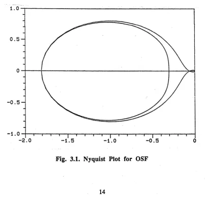
The former is stable and the latter has two unstable poles. Figure 3.1 shows the
Nyquist plot.
0 . 5
0 . 5
-- 1 . 0
[image:38.523.56.466.374.765.2]CH 2 LOOP RECOVERY
0 . 5
0 . 5
-- 1 . 0
- 0 . 5
- 1 . 0
- 1 . 5
- 2 . 0
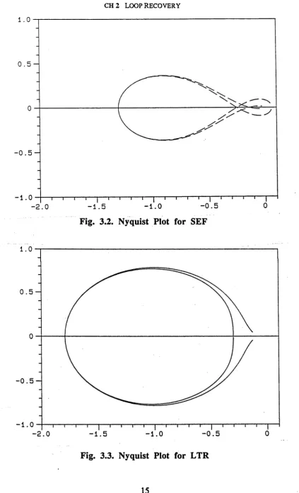
Fig. 3.2. Nyquist Plot for SEF
0 . 5
0 . 5
-- 1 . 0
- 0 . 5
- 2 . 0 - 1 . 5 - 1 . 0
[image:39.523.52.476.56.753.2]CH 2 LOOP RECOVERY
Now the state estimator is designed with Ki = 0, K° = [-3.6 0.9 0.2]x. Figure 3.2
shows the associated Nyquist plot with relatively poor robustness properties.
Choose vf = N(0, 10000) to recover the outer state feedback loop robustness, now
K1 = 0, K° = [68.1 11.7 0.8]x and Figure 3.3 shows the loop recovery.
4. Frequency Shaped Estimation
When plant input noise is colored, rather than white as in the standard estimator
theory, then it is straightforward to augment the plant model with the noise model
and apply standard filter theory to the augmented plant However, as the theory of
[6] illustrates, the formulations and proof techniques are awkward. Here a direct
approach in the frequency domain is taken so as to achieve the simplicity of
derivation and formulation of the results of Section 2, which are essential for the
frequency shaped loop recovery theory of Section 2.
Noise model Plant
Fig. 4.1. Signal Model
Signal Model:
[image:40.523.38.450.448.688.2]CH 2 LOOP RECOVERY
white noise sources with zero means and covariances I, R = Rx > 0 respectively.
2
The plant input vct is colored noise with a spectrum Q(s) where Q (s? is a stable
minimum phase spectral factor of Q(s). The plant state model has a (strictly proper)
transfer function W(s)=C(sI-A)_1 for some (A,C) observable. The plant is possibly
unstable. Its output is zt. For subsequent results, Q(s) must be such that
W(s)Q(s)W(-s)x has no hidden jco axis modes.
Spectral Factorization:
Consider a spectral factorization of the spectrum of zt as follows:
W(s)Q(s)W(-s)x+R = F(s)FT(-s), F(s) = [I+W0l(s)]R^ (4.1)
2
where F(s), Wq l(s) have the same poles as W(s)Q(s)2 and the spectral factor F(s)
is minimum phase. In [10], this factorization is carried out for a dual control
situation. First W is expressed as a matrix fraction decom position
W = with M, N e RH°° (rational proper asymptotically stable). Then
N(s)Q(s)N(-s)x - M(s)RM(-s)x = S(s)S(-s)x is factorized to achieve S(s) (strictly)
minimum phase and asymptotically stable under the assumption above. Next
W0L(s) and F(s) are given from
W0l(s) = M(s)-'S(s)R -L I, F(s) = CT(s)-!S(s)
I
As shown in [10]. Wo l(s) is unique strictly proper (strictly) minimum phase, and
has the following properties.
Lemma 2: With Wol(s) given from the spectral factorization (4.1), under the
restrictions on W(s), Q(s), R above, with C'R a right inverse of C there exists
CH 2 LOOP RECOVERY
W(s)K(s) = Wq l(s) , (4.2)
Moreover, there exists some rational P(s) such that [with X* 4 X(-s)T]
(I + WK)_1WPC g RH°°
(s-1P)[(sI-A) + KCM(sI-A) + KC](s-1?)* = KPK* + Q
WK = W(s"1P)CTR‘1
W [(s'1P)(sI-A)*+(sI-A)(s'1P)*+(s'1P)CrR '1C (s'1P)*-Q]W*=0 (4.3)
Optimal Estimation:
Consider the filter arrangement of Figure 4.2, which is asymptotically stable since
under Lemma 2, K(s) stabilizes W(s) in feedback. Then it is immediate from the
spectral factorization (4.1) that vt is white zero mean and has a covariance R. It
follows from the inverse problem of optimal filtering [13] that yk is indeed the
optimal filtered estimate of yt in a least squares sense. Moreover, with [A,C]
completely observable, a mild generalization of the argument in [13] gives that Xk is
the optimal state estimate.
[image:42.523.50.473.556.783.2]CH 2 LOOP RECOVERY
5. Conclusions
The technique of loop recovery for improved robustness in state estimate feedback
designs generalizes to cope with nonminimum phase plants. A generalization
restricts the class of state feedback controllers to those which feedback only the
state (or estimates) associated with the "minimum phase" states in an all
pass/minimum-phase factored signal model form. Of course, for some
nonminimum phase plants, such controllers are not expected to achieve robust
designs comparable to those for minimum phase plants. However, whatever loop
robustness is achieved in such a partial state feedback design is recovered in a state
estimate feedback design using the loop recovery techniques of this chapter. One
specific method for a stabilizing partial state feedback design has been presented
and a design example has been included to illustrate the approach. Also the results
for frequency shaped state estimators have been developed.
References
[1] B.D.O. Anderson and J.B. Moore, "Linear Optimal Control", Prentice Hall, 1971.
[2] H. Kwakemaak and R. Sivan, "Linear Optimal Control Systems",
Wiley, New York, 1972.
[3] M.G. Safonov and M. Athans, "Gain Phase Margins for Multiloop LQG
CH 2 LOOP RECOVERY
[4] J.C. Doyle, "Guaranteed Margins for LQG Regulators", IEEE Trans. Auto. Control, Vol.AC-23, No.4, pp756-757, August 1977.
[5] J.C. Doyle and G. Stein, "Robustness with Observers", IEEE Trans. Auto. Control, Vol.AC-24, No.4, pp607-611, August 1979.
[6] J.B. Moore, D. Gangsaas, J.D. Blight, "Performance and Robustness
Trades in LQG Regulation Design", Proceedings of 20th Conference on Dec. and Control, San Diego p p l 191-1200. December 1981.
[7] B.A. Francis, J. Helton and G. Zames, "H°°-Optimal feedback controller
for linear mulitvariable systems", IEEE Trans. Vol. AC-29 pp.888- 900.
[81 J.B. Moore, L. Xia and K. Glover, "On improving Control Loop
Robustness of Model Matching Controllers", Systems and Control Letters 7 (1986) pp. 83-87.
[9] J.B. Moore, K. Glover and A. Telford "On the Class of all Stabilizing
Controllers", Proc. of Conference on Dec. and Control, Athens, Dec. 1986.
[10] J.B. Moore, "Robust Frequency Shaped LQ Control", submitted to
Automatica.
[11] C. Chu and J. Doyle, "On Inner-outer and Spectral Factorizations",
Proceedings of 23rd Conference on Dec. and Control, Los
CH 2 LOOP RECOVERY
[12] K. Glover, "All optimal Hankel-norm approximations of linear
multivariable systems and their L°°-error bounds", Int.J. Control
Vol.39. No.6, pp 1115-1193.
Chapter 3
On Improving Control
-Loop robustness
ofmodel matching
C
ontrollers1 In t r o d u c t io n
In seeking robust controllers, H°°-methods search over the (infinite) class of all
stabilizing transfer function controllers for one that minimizes some L°°-sensitivity
measure. A key observation is that such problems can be reduced to solving a
Nehari H°°-optimization of an L°°-norm, [l]-[5]. Appropriate generalizations of the
fundamental results using more general indices [6] including frequency shaped
indices [4], potentially lead to practical designs.
Here, a class of stabilizing two-degree-of-freedom controllers which achieve a
specified (achievable) closed loop transfer function is conveniently characterized.
Also, the search over this class of controllers for one which has optimum open loop
robustness properties in an L°°-sense is shown to reduce to solving a standard
H°°-optimization problem.
The a priori specification of a desired transfer function could arise, for example,
from an optimal linear quadratic Gaussian (LQG) design, or some other standard
method applied to the nominal plant Referring to Figure 1, a preliminary design for
a plant P(s) could give proper controllers K°(s) = [Ki°(s) K2°(s)] which achieve
desired closed loop transfer function properties for the nominal plant but which
have poor open loop robustness properties, as measured by the L°°-norm
CH 3 MODEL MATCHING CONTROLLERS
chapter then allow the definitions of a comprehensive class of controllers K(Q,s) in
terms of an arbitrary Q(s) e RH°° (proper stable transfer function), so that the
closed loop transfer function is invariant of Q(s). This allows the selection of a
specific Q(s), denoted Q0pt(s), to minimize the index
III + P(s)K2(Q,s) lloo
or a related measure. The controller K(Qopt,s) achieves the desired closed loop
transfer function for the nominal plant P(s) and improves open loop robustness.
K (s)
'[^ (S ) K2(s)] P fcLr I5r
Figure 1. Control System with two-degree-freedom Controller
2. The Class of Stabilizing Controllers
Consider the class of two-degree-of-freedom controllers of Figure 1 where P(s) is
the plant and K(s) = [Ki(s) K2(s)] e Rp (rational proper transfer function) is the
controller. The controller is said to be stabilizing when all transfer functions
between variables are stable. When Ki(s) = I, then the controller has one degree of
freedom and is stabilizing if and only if
CH 3 MODEL MATCHING CONTROLLERS
(I + PK2)-!P g RH°° , I - K2(I + PK2)-!p G RH°° (2.1) The class of such controllers is given in terms of an arbitrary stable Q(s) as in [7]:
K2(Q) = (U - MQ)(V + NQ)-1, Q € RH°°
P = N M -!=M -1N, VM + ÜN = I, ftU + MV = I,
M, N, TM, N, U, V, Ü, V g RH°° (2.2)
Lemma 2.1 The class of two-degree-of-freedom controllers
K(s) = [Ki(s) K2(s)] for the plant P(s), as in Figure 1, is stabilizing if and
only if
K2(s) is stabilizing as one-degree-of-freedom controller for P(s)
[namely (2.1) hold] (2.3a)
Ti 4 (I + K2P)-!Ki g RH~,
T2 4 P(I + K2P)-!Ki g RH°° (2.3b)
Proof: All of the possible transfer functions between variables are given by those
in (2.1) and (2.3) or are trivially related to those using the standard identity
(I + XY)-lX = X(I + YX)-1. AAA
Remarks 1. Observe that if the controller is realized as two separate controllers, as
is often the case in a classical servo design, then in addition, (2.3) would include
the condition Ki(s) g RH°°, details are omitted.
CH 3 MODEL MATCHING CONTROLLERS
K (s) = [K i(s) K2(s)] for the plant P(s), can be characterized in terms o f two
arbitrary transfer functions, Q i(s), Q(s) e RH°° as follow s, see also [8].
Characterize the matrix K2(s) in terms o f arbitrary Q(s) e RH°° as in (2.2), and
K i(s) in terms o f arbitrary Q i(s) e RH°° as
K i = (M + K2N)Qi, Qi e RH°° (2.4)
A proof is as follows. From (2.4), and since M, N e RH°°,
Ti 4 (I + K2P)-1Ki = MQi € RH°°
T2 4 Pa + K2P)-1Ki = NQi e RH°°
and (2.3b) holds. From (2.2) then (2.3a) holds. Applying Lemma 2.1 then
K = [K i K2] defined from (2.2) and (2.4) is stabilizing. Also, given arbitrary
stabilizing K = [K i K2] for P, then K2 is given from (2.2) in terms o f arbitrary
Q e RH°°. Now define
Ql = M-1(I + KP)_1Ki
with M from (2.2). This has the property that [M N]Qi € RH°° with K2 stabilizing
and N also from (2.2). Since M, N are coprime, then Qi e RH°°. Now (2.4) holds
trivially.
3. A Class of Model Matching Controllers
To motivate the following results, let us consider that a two-degree-of-freedom
CH 3 MODEL MATCHING CONTROLLERS
requirements for the nominal plant P with
Ti* 4 (I + K2*P)-1Ki* e RH°°
T2* 4 P(I + K2*P)_1Ki* e RH°° (3.1)
Let us seek result which allow improvement of loop robustness of such a design
while keeping the transfer functions Ti*(s), T2*(s) invariant of any adjustments
made to Ki, K2.
The design technique to achieve Ti*(s), T2*(s) is not important for our theory.
However we could have in mind an optimal LQG design using a performance index
with engineering significance. Often such designs results in poor robustness to
plant uncertainty, in which case the following results could be useful.
Lemma 3.1 Consider the class of two-degree-of-freedom controllers
K(s) = [Ki(s) K2(s)] e Rp
for the plant P(s) as in Figure 1. Necessary and sufficient conditions for
K = [Ki K2] to match the model transfer functions (3.1) and be stabilizing
are that
Ki = (I + K2P)(I + K2*P)-lKi* = Ti* + K2T2* (3.2a)
K2 as one-degree-of-freedom controller for P(s) is stabilizing. (3.2b)
Moreover, the entire class of such stabilizing controllers can be characterized
in terms of arbitrary stabilizing K2 as a one-degree-of-freedom controller for
CH 3 MODEL MATCHING CONTROLLERS
arbitrary Q e RH°° as in (2.2). Furthermore, closed loop transfer functions
are affine in Q.
Plant
Plant
Plant model
Fig. 2. Model Matching Controllers.
Proof A necessary condition for model matching is that
Ti = (I + K2P)_1Ki = a + K2*P)-1Ki* b Ti* (3.3a)
which is equivalent to (3.2a). Now (3.3a) implies that
T2 = P(I + K2P)-!Ki = P a + K2*P)"*Ki* ■ T2* (3.3b)
and so (3.2a) is also sufficient for model matching. Clearly, (3.2b) is necessary for
stability. Also, the property (3.2), together with (3.1) ensure that the model
[image:51.523.50.457.135.643.2]CH 3 MODEL MATCHING CONTROLLERS
The structure of Figure 2 is verified since its transfer function is
P(I + K2P)-1Ti* + PK2(I + p k2)-i t2*
= P(I + K2P)-1(Ti* + K2T2*)
= P(I + K2P)-1Ki = T2*
which is invariant of K2 given that K2 is stabilizing. Now substituting Ki from
(3.2a) into (2.3b), and applying (2.1), (2.2) the remaining results are obtained.
AAA
Remarks 1. For the controllers of Figure 2, robustness properties are crucially
dependent on K2. Observe that for the nominal plant and zero initial conditions, the
input to the block K2 is zero since its transform is
T2*(s)u(s) - y(s)
Where y(s) = T2*(s)u(s). In this case then the control is essentially feed-forward
control and independent of K2. Otherwise, the greater the gain K2 at a particular
frequency, the more significant is the feedback control via K2 at that frequency.
2. In any realization of K = [Ki K2], it is important to avoid duplication of an
unstable mode. For example, if Ki(s), K2(s) were realized as separate controllers
as in classical designs, then any unstable poles in K2 that are also in Ki would give
closed loop instability. In the schemes of Figure 2, any instability is confined
within a stable closed loop.
3. The schemes of Figure2 are in terms of an arbitrary stabilizing K2 for the plant