Model term selection for spatio-temporal system identification using mutual information

This is a repository copy of Model term selection for spatio-temporal system identification using mutual information.

White Rose Research Online URL for this paper: http://eprints.whiterose.ac.uk/74664/

Monograph:

Wang, S., Wei, H.L., Coca, D. et al. (1 more author) (2010) Model term selection for spatio-temporal system identification using mutual information. Research Report. ACSE Research Report no. 1013 . Automatic Control and Systems Engineering, University of Sheffield

eprints@whiterose.ac.uk https://eprints.whiterose.ac.uk/ Reuse

Unless indicated otherwise, fulltext items are protected by copyright with all rights reserved. The copyright exception in section 29 of the Copyright, Designs and Patents Act 1988 allows the making of a single copy solely for the purpose of non-commercial research or private study within the limits of fair dealing. The publisher or other rights-holder may allow further reproduction and re-use of this version - refer to the White Rose Research Online record for this item. Where records identify the publisher as the copyright holder, users can verify any specific terms of use on the publisher’s website.

Takedown

If you consider content in White Rose Research Online to be in breach of UK law, please notify us by

Model Term Selection for Spatio-temporal

System Identification using Mutual Information

Shu Wang, Hua-Liang Wei, Daniel Coca and Stephen A. Billings

Research Report No. 1013

Department of Automatic Control and Systems Engineering

The University of Sheffield Mappin Street, Sheffield,

S1 3JD, UK

Model Term Selection for Spatio-temporal

System Identification using Mutual Information

Shu Wang, Hua-Liang Wei, Daniel Coca and Stephen A. Billings

Department of Automatic Control and Systems Engineering, University of Sheffield, Mappin Street, Sheffield S1 3JD, UK

Abstract

A new mutual information based algorithm is introduced for term se-lection in spatio-temporal models. A generalised cross validation procedure is also introduced for model length determination and examples based on cellular automata, coupled map lattice and partial differential equations are described.

1

Introduction

Spatio-temporal systems represent a class of complex dynamic systems, which contain both time and space information. The study of spatio-temporal systems may help to decipher many spatio-temporal phenomena and behaviours that ap-pear in nature and to better understand and possibly control the formation of spatio-temporal patterns[20][4][21].

One of the key concerns in the analysis of spatio-tempotal systems is system identification, the reverse problem of pattern formation, which is still an open problem. One of main tasks in spatio-temporal system identification is model structure selection which enables construction of a mathematical model from ex-perimental data. The Orthogonal Forward Regression (OFR) algorithm is one of the effective methods for the identification for spatio-temporal systems. Given a large number of candidate model terms in an initial model, this algorithm can be used to determine which terms or regressors are significant and should be included in the model based on the Error Reduction Ratio (ERR)[7][9]. However, when applied to some spatio-temporal data sets the OFR algorithm can occasionally select some spurious model terms, which can then result in a comparatively more complex model with some possible insignificant or redundant model terms.

2

Spatio-temporal model description

This study considers three main types of spatio-temporal models: Cellular Auto-mata or simply CA, Coupled Map Lattices (CML), and Partial Differential Equa-tions (PDE). CA are systems that have finite values at each cell site and the rules are usually represented by a combination of different Boolean rules. The class of systems that have continuous state cell values at each site can be described by Partial Differential Equations (PDE), or when based on a discrete lattice space as Lattice Dynamical System (LSD) or Coupled Map Lattices (CML). However, LSD, CML and CA models have the property of discrete space, but PDE models not only have a continuous state, but also continuous time and space.

2.1

Cellular Automata

Cellular Automata (CA) were initially introduced by von Neumann in the early 1950’s. CA are dynamical systems in which space and time are both discrete. Each cell which is arranged in the form of a regular lattice structure has a finite number of states. All the states in the cells are updated synchronously by a specific transition rule based on the information of the individual states and of cells in a neighbourhood at past times.

An n-dimensional cellular automata is defined on a lattice structure. The typical and widely used lattice type is a square lattice, which is represented as

Sd_{, where d = 2r+ 1 ,and r is a finite integer which determines the size of the}

neighbourhood. S is a finite set of states of all cells in the lattice. The dynamics are described by a neighbourhood function f : Sd _{→ S. Thus, the output of}

each cell is produced by following the rule f. The transition function f shows the interaction of cells which can be listed in a finite look-up table. A shift operator then upgrades the cells as time passes.

Consider a one-dimensional 3-site CA model, the spatio-temporal patterns ge-nerated by 100 time steps evolution are shown in Figure 1. In the simulation, 100 random data valued 1 or 0 are set as initialization. The neighbourhood was set as {c(j−1;t), c(j;t), c(j+ 1;t)}, wherec(j, t) indicates the cell state at the position

j and the time instantt . The transition rule described by the Boolean equivalent is

c(j; t+ 1) =c(j; t)∨(c(j −1;t)∧c(j+ 1;t)) (1) where ′

∨′

denotes the OR operation and ′ ∧′

denotes the AND operation. It has been shown in [6] that CA rules can be expressed in a polynomial form for the model in Equation (1), gives

c(j,t+ 1) = −2.0c(j−1;t)c(j;t)−2.0c(j;t)c(j+ 1;t) +c(j;t) −2.0c(j−1;t)c(j+ 1;t) +c(j−1;t)

+3.0c(j −1;t)c(j;t)c(j + 1;t) +c(j+ 1;t) (2)

2.2

Coupled Map Lattice

Figure 1: The CA model simulation for equation (2)

The CML model is a typical model of extended dynamical systems with discrete time and space, but with continuous state variables. The CML model lies somew-here between CA and PDE models. CML models are convenient for computer simulations especially of physical systems, for the interpretation of experimental results, and for mathematical analysis.

There are four key parts in CML models, that is, a lattice structure, the neigh-bourhood, the lattice states and a dynamical process. The process of a CML model can be defined by the following parts [12]:

• A lattice architecture.

Let x be a cell in a lattice X, so that x ∈ X . The neighbourhood can be described as

N hd(x) ={x, yp(x)

x } (3)

where y represents the neighbouring cells corresponding to the cell x. p(x) represents the selection of neighbourhood cells and also specifies the size of the neighbourhood.

• Lattice state description.

The mapping for the state of lattice is η : X → A, where A describes the states in the lattice. Thus, the state of a cell x in a lattice can be described asη(x).

• Dynamic process.

There are two basic processes involved: isolated local processes and interac-tion processes. For an isolated local mappingfx : A→M ,M is the set of all possible values of cells in a lattice, andfx(a)shows the output value at point

xwhen the input value is a. Unlike the isolated process, the interaction pro-cess couples the states generated from the cells in the neighbourhood. This is represented by gx : Mp(x) _{→ A. A global description of such a dynamic}

process was expressed by Holden [12], Vx : T ×[X →A]→A, where T is a time delay matrix. Vx(0, η) = η(x) when t= 0, so for t >0,

Vx(t+ 1, η) = gx(fx(Vx(0, η)), fyx,1(Vyx,1(t, η)),. . ., fyx,p(x)−1(Vyx,p(x)−1(t, η))) (4)

Consider an example of the CML model proposed by Sole and Valls [23]:

(a) xi(t) (b)yi(t)

Figure 2: Original CML model simulated patterns for Eqns (5) and (6).

yi(t) =xi(t−1){1−exp[−βyi(t−1)]}+D2∇2yi(t−1) (6)

wherei= (i1, i2)∈Z2, describes the cell location in the lattice. ∇2 is the Laplace

operator and can be given by

∇2xi1,i2(t−1) = xi1−1,i2(t−1)+xi1+1,i2(t−1)+xi1,i2−1(t−1)+xi1,i2+1(t−1)−4xi1,i2(t−1) (7) This system with µ = 4, β = 5, D1 = 0.001, D2 = 0.2 was simulated on a

lattice of 256×256 with 50 random initial seeds of values between 0.3 to 0.4 [23] and periodic boundary conditions. The simulation results for 2000 time steps are show in Figure 2.

2.3

Partial Differential Equations Models

PDE models are continuous in both the time and space domains, and also conti-nuous in the state at each point. With these conticonti-nuous properties, PDE models provide an effective tool to understand and reconstruct continuous spatio-temporal systems in the real world. It is because these models may be related to previously derived analytical PDE models so that there is the potential to provide a clear physical explanation of the underlying system properties. PDE models demons-trate a relation between an unknown function with several independent variables and the associated partial derivatives. The general form of a PDE model based on a functionu(x1, x2, . . . , xn) is

F(x1, x2, . . . , xn, u, ux1, ux2, . . . , ux11, . . .) = 0 (8)

wherex1, x2, . . . , xn are the independent variables,uis the unknown function, and

uxi represent the partial derivatives

∂u

∂xi. Generally, additional conditions such as initial conditions and boundary conditions are included. One example of a PDE model is the model of the streaming movement in a colonization period of bacterial cells [14]

∂n ∂t =∇

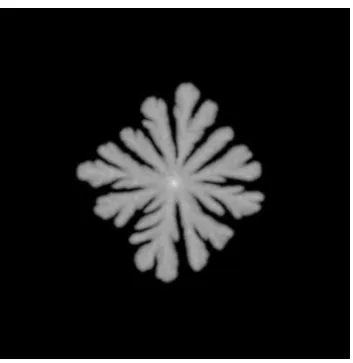
Figure 3: The simulation of bacterial population b in PDE models for Eqns (9) and (10).

∂b

∂t =∇ · {σnb∇b}+nb (10)

where n and b represent the concentration of the nutrient and the population density of the bacterial cells respectively. Here σ = σ0(1 + ∆), σ is random and

normally distributed with the mean σ0. Computer simulations of equations (9)

and (10) were applied on the space domain (0,1)×(0,1) and over a lattice with the size of 400×400 and no-flux boundary conditions. For the initialization, the bacterial cells were distributed in a round-shaped area in the center. The initial distribution can be described as below,

bi(0) =βi1,i2(0) =βMexp{−(i

2

1+i22)/6.25} (11)

where βM represents the maximum density. The nutrient was evenly distributed at a level n0.

The simulation results for 8000 steps with βM = 0.71, n0 = 0.35, σ0 = 4 are

show in Figure 3.

3

Identification of Spatio-temporal models using

the OLS algorithm

Many non-linear dynamic systems can be represented by the NARMAX model, (Non-linear Auto Regressive Moving Average with eXogenous inputs)[15], which is defined as

y(t) = F(y(t−1),. . ., y(t−ny), u(t−1),. . ., u(t−nu), e(t−1),. . ., e(t−ne)) +e(t) (12) where y(t), u(t) and e(t) represent the output, input and noise sequences res-pectively. When this model is extended to the MIMO case with m variables in the system output and r variables in the input, the variables can be written as vectors y(t) = [y1(t), y2(t), . . ., ym(t)]T, u(t) = [u1(t), u2(t),. . ., ur(t)]T and

e(t) = (e1(t), e2(t),. . . ,em(t))T. ny, nu and ne are the maximum time delay, e(t)

objective of system identification is to find a proper approximation with respect to F. A common choice is to describe F by a polynomial representation with a given degreel,

y(t) = θ0+

n

X

i1=1

θi1Ti1(t) +

n

X

i1=1

n

X

i1=i2

θi1,i2Ti1(t)Ti2(t) +· · ·

+

n

X

i1=1 · · ·

n

X

il=il−1

θi1...ilTi1(t)· · ·Til(t) +e(t) (13)

where n = ny +nu +ne and T(t) represents y, u or e with time lags. Equation (13) can be written as a linear in the parameters regression model

y(t) =

M

X

i=1

θixi(t) +ξ(t), t= 1, . . . , N (14)

where N is the data length. θi are unknown parameters to be estimated. xi(t) are model terms from the combination ofT(t)up to degree l,M is the number of terms involved in this system, and ξ(t) is the modelling error.

An optimized identified model should contain all the significant terms in equa-tion (14), and all the redundant terms should have been removed from the model. The orthogonal least squares (OLS), also known as the orthogonal forward regres-sion (OFR) algorithm with error reduction ratio (ERR) has proved to be one of the most efficient methods for term selection and parameter estimation in nonlinear temporal system identification [7][9][8][1][2]. This method was initially applied to single-input single-output (SISO) systems, but it has been widely extended to many multi-input multi-output (MIMO) systems.

The Orthogonal forward regression (OFR) algorithm is based on the orthogo-nalization of regressors which are the terms in models. The classical orthogonal forward regression algorithm results in a particularly simple estimation procedure which is described by the following steps:

1. Orthogonalize all the regressors in a model so that the correlations between all the terms are removed.

2. Determine significant terms using the error reduction ratio (ERR).

3. Estimate the corresponding parameters with respect to the selected terms.

4

The New OFR-MI algorithm

4.1

Mutual Information

Mutual Information (MI) which was initially proposed by Shannon in 1948 [22], is one of the effective measurements of the similarity between two variables. If two variables are strictly independent, the MI between the two variables should be zero.

I(x,y) = X

x∈X

X

y∈Y

p(x,y) log( p(x,y)

p(x)p(y)) (15)

For the specific example of the model in Equation (14), wherey is the output and xi is one of the orthogonal regressors in the model, the mutual information

I(xi, y)betweenxi and ymeasures how a knowledge ofxi reduces the uncertainty about y, or the information that xi and y share. Hence, the regressor xi with the biggest MI value may make the most contribution to the model. Thus, Mutual Information incorporated with an orthogonalisation procedure can be used as an alternative to the ERR term selection procedure in the classical OFR algrithm to aid the selection of significant model terms.

Several algorithms have been developed to estimate mutual information from observed data, including the approach using a histogram based technique [10][16], methods based on kernel density estimators [18], and parametric methods [11]. In this work, the adaptive histogram-based method proposed in [10] is employed, because this method is applicable to any distribution and appears to be asympto-tically unbiased and efficient[25].

4.2

The New OFR-MI algorithm

Mutual information will be added into the OLS algorithm’s orthogonalisation pro-cedure as a criterion to decide the significance of model terms instead of using the ERRs [26]. According to Equation (14), The algrithm can be described as follows.

1. (a) Step 1. All the model terms X1 = xi(t), i = 1, . . . , M are candidates

for the important term w1(t). For i= 1, . . . , M,

w(₁i)(t) = xi(t), [M I](₁i)(y(t), xi(t)) =X

y∈Y

X

xi∈X

p(y,xi) log( p(y,xi)

p(y)p(xi))

whereY =y(t). Find the maximun of[M I](1i), say,[M I] (j)

1 =max{[M I] (i) 1 ,1≤

i ≤ M}. The first significant terms can be w1(t) = w(

j)

1 (t), xj(t) is

se-lected with

y1(t) =y(t)−

y(t)w1(t)

w2 1(t)

w1(t), α11= 1, gˆ1 =

w1(t)y(t)

w12(t)

, M I1 = [M I](

j) 1

and the error-to-signal ratio (ESR), which is used as the criterion to

ter-minate the search procedure, iskr1k2 =

ky1k2

kyk2 = (kyk

2₋(yw1)2

w₁2 )/kyk

2_.

(b) Step 2. All the rest of the terms X2 = xi(t), i = 1, . . . , M, i 6= j form

the candidate terms for w2(t), For i= 1, . . . , M, i6=j,

w₂(i)(t) = xi(t)−α(₁₂i)w1(t),

[M I](₂i)(y1(t), xi(t)) = X

y1∈Y₁

X

xi∈X1

p(y1,xi) log(

p(y1,xi)

p(y1)p(xi)

)

where

α(₁₂i) = w1(t)xi(t)

Find the maximun of [M I](₂i), [M I](₂k) = max{[M I](₂i), 1 ≤i ≤ M, i6=

j}. Then the second basisw2(t) =w2(k)(t), xk(t)is selected with

y2(t) = y1(t)−

y1(t)w2(t)

w2 2(t)

w2(t), a22= 1, a12=a(12k),

ˆ

g2 =

w(₂k)(t)y(t)

w(2k)(t)

2, M I2 = [M I] (k) 2

and the ESR is kr2k2 =

ky2k2

kyk2 = (ky1k

2₋ (y1w2)2

w₂2 )/kyk

2_.

(c) This procedure is terminated at the Msth step when eitherkrMsk

2 _{< ρ}

or Ms =M, whereρ is a desired stopping tolerance.

2. Compute the estimated paremeters θiˆ

ˆ

θM = ˆgMs;

ˆ

θ = ˆgi−

Ms

X

k=i+1

αikθk,ˆ i=Ms−1, . . . ,1

4.3

Model length determination

In practice, an identified model from real data can be either overfitting or under-fitting, which may cause the model lacks good generalization properties. Thus, the validation of selected model terms and the final model is important. One of the effective methods to refine the model is cross validation [24][8][1][2], a tool that can be used to detemine model size. Generalised cross-validation (GCV) is one type of cross validation, that is commonly and widely used. The GCV criterion used for linear regression model [19][3] can be expressed

GCV (n) =

N N −n

2

M SE(n) (16)

where N is the length of the test data set, n is the number of selected model terms and the Mean-Square-Error (MSE) is M SE(n) = krnk2_{/N corresponding}

to a model with n terms [26][5]. GCV will have a minimum value when n is the effective number of model terms [17].

5

Examples

In this section, several identification examples for spatio-temporal systems using both OFR and OFR-MI algrithms will be described. It is shown that OFR-MI produces good results for selecting the correct terms for spatio-temporal model identification.

5.1

CA model Identification

Table 1: Identified model structure for the CA model of Eqn.(2) using OFR algorithm

Terms Parameters ERR(%) GCV

Ture Estimated

1 0 -5.4401E-15 35.71 0.6431

c(j−1;t)c(j;t) -2.0 -2.0 8.36 0.5595

c(j −1;t) 1.0 1.0 7.6 0.4836

c(j−1;t)c(j + 1;t) -2.0 -2.0 2.83 0.4554

c(j+ 1;t) 1.0 1.0 7.0 0.3854

c(j−1;t)c(j;t)c(j+ 1;t) 3.0 3.0 4.82 0.3373

c(j;t)c(j+ 1;t) -2.0 -2.0 14.18 0.1954

c(j;t) 1.0 1.0 19.51 0.0

Table 2: Identified model structure for the CA model of Eqn.(2) using OFR-MI algorithm

Terms Parameters MI GCV

Ture Estimated

c(j−1;t)c(j;t) -2.0 -2.0 0.1383 0.3571

c(j;t)c(j+ 1;t) -2.0 -2.0 0.2114 0.3572

c(j;t) 1.0 1.0 0.3108 0.2916

c(j−1;t)c(j+ 1;t) -2.0 -2.0 1.5207 0.2830

c(j−1;t)c(j;t)c(j+1;t) 3.0 3.0 1.6856 0.2696

c(j−1;t) 1.0 1.0 0.3008 0.1348

c(j + 1;t) 1.0 1.0 0.57 1.84E-16

Table 1 shows that a constant term is selected by the OFR algorithm with the highest ERR value. However, this term should not be in the model. Table 2

shows the results produced by the new OFR-MI algorithm. All the seven selected terms are exactly consistent with the true model terms. In addition, it shows that identified model enables the GCV value to be minimised.

5.2

CML model Identification

The CML model described in Section 2.2 was simulated. The identification was performed using data from eight points at locations (200,192), (200,193), (200,194), (200,195), (200,196), (200,197), (200,198), and (200,199) over 500 time steps. The data length is therefore 8×500. The final models identified from the data are detailed in Tables 3 and 4.

Table 3: Identified model structure for the CML model of Eqns (5) and (6) using OFR algorithm

Output Terms Parameters ERR(%) GCV

Ture Estimated

x(t) x(t−1)[1−x(t−1)] exp[−βy(t−1)] 4.0 4.0 99.999988345 1.1661E-7

∇2_{x 0.001 0.001 1.1655E-5 0.0}

y(t) x(t−1) 1.0 1.0 88.82 0.1119

x(t−1) exp[−βyi(t−1)] -1.0 -1.0 10.78 0.004

∇2_{y 0.2 0.2 0.4 2.2238E-16}

x(t−1) exp[−βyi(t−1)]∇2_{y 0 3.2513E-14 4.0235E-30 2.2249E-16} exp[−βyi(t−1)] 0 6.0457E-17 2.1667E-30 2.2260E-16 x(t−1)∇2_{y 0 -1.5438E-14 2.7343E-30 2.2271E-16} exp[−βyi(t−1)]∇2_{y 0 -7.7381E-15 8.4522E-30 2.2283E-16}

Table 4: Identified model structure for the CML model of Eqns (5) and (6) using OFR-MI algorithm

Output Terms Parameters MI GCV

Ture Estimatied

x(t) x(t−1)[1−x(t−1)] exp[−βy(t−1)] 4.0 4.0 7.1866 1.4796E-08

∇2_{x 0.001 0.001 6.2765 0.0}

y(t) x(t−1) 1.0 1.0 2.6799 0.0039

x(t−1) exp[−βyi(t−1)] -1.0 -1.0 3.8430 1.3961E-04

∇2_{y 0.2 0.2 5.4032 8.7180E-18}

almost the same amplitude because of the high sampling. This problem exists in the models studied here but reducing the sampling was not found to be an effective solution.

However, the new OFR-MI algorithm can effectively avoid the problem of high initial ERR values. From Table 4, the estimated terms are identical to the true model terms.

5.3

PDE models

Table 5: Identified model structure for the PDE model of Eqns (9) and (10) using OFR algorithm

Output Terms Parameters ERR(%) GCV

Ture Estimated

n(t) n(t−1) 1.0 1.0 99.96 3.7533E-4

b(t−1)n(t−1) -0.2 -0.2 2.5720E-2 1.1810E-4 ∇2_{n 0.2 0.2 1.1804E-2 1.4444E-15}

b(t) b(t−1) 1.0 1.0 99.99931422 6.8595E-6

σb(t−1)n(t−1) 0 -2.3822E-13 5.2959E-4 1.5627E-6

σb(t−1)n(t−1)∇2_{b 2.0 2.0 1.0804E-4 4.8185E-7}

∇(σnb)∇b 2.0 2.0 4.1976E-5 6.1797E-8

b(t−1)n(t−1) 2.0 2.0 6.1735E-6 0.0

Table 6: Identified model structure for the PDE model of Eqns (9) and (10)using OFR-MI algorithm

Output Terms Parameters MI GCV

Ture Estimated

n(t) ∇2_{n 0.2 0.2 3.9504 0.0033}

n(t−1) 1 1 6.2936 1.0237E-6

b(t−1)n(t−1) -0.2 -0.2 13.3318 4.8288E-19

b(t) n(t−1)∇(σnb)∇b 0 -5.2225E-13 6.388 0.5180

σn(t−1) 0 -1.6653E-16 8.0544 0.5139

b(t−1)n(t−1)∇2_{b 0 9.4502E-13 4.3195 0.5094}

b(t−1)n(t−1) 0.2 0.2 6.8711 0.4869

σb(t−1)n(t−1)∇2_{b 0.2 0.2 3.9573 0.4853}

b(t−1) 1.0 1.0 2.6855 2.9212E-8 ∇(σnb)∇b 0.2 0.2 1.2248 0.0

From Table 5, the ERRs of the first terms, ni(t−1) and bi(t −1), for both

n(t) and b(t) are close to 1.0 using the OFR algorithm. As noted above this may be caused by the high sampling frequency, so that the output values at the time step t−1 are almost identical to the ones at t step. Hence, the terms at

t−1 time step are selected as the first term every time. If the spurious terms are included in the model, poor estimations may be resulted. However, if the sampling frequency is reduced, the correct models may not be correctly detected. This problem appears to be important in spatio-temporal system modelling. The OFR-MI algorithm overcomes these problems and is applicable for spatio-temporal system identification. However, the OFR-MI algorithm can not always produce better results than the OFR algorithm. For example, the results in Table 6, for the model of n(t), all the right terms have been detected. But for the model of

6

Conclusions

The new OFR-MI algorithm provides an effective model term selection approach for spatio-temporal system identification. In some spatio-temporal system cases spurious terms may be detected using the classical OFR algorithm due to high initial ERR values. This means that the subsequent selection precedure based on ERR values can be affected by the spurious terms. However, by using the new OFR-MI algorithm, this problem can be overcome, because the mutual information is introduced as a criterion for the term selection, which works as a replacement of the ERR precedure in the OFR algorithm. The OFR-MI algorithm works well on spatio-temporal models including CA, CML and PDE models. The OFR-MI algorithm is therefore a complementary method for the OFR algorithm, rather than a substitute.

Acknowledgements

The authors gratefully acknowledge that this work was supported by University of Sheffield, EPSRC(UK) and the European Research Council.

References

[1] L. A. Aguirre and S. A. Billings. Validating identified nonlinear models with chaotic dynamics. International Journal of Bifurcation and Chaos, 4(1):109– 125, 1994.

[2] L. A. Aguirre and S. A. Billings. Dynamical effects of overparametrization in nonlinear models. Physica D: Nonlinear Phenomena, 80(1-2):26–40, Jan. 1995.

[3] M. Alan. Subset Selection in Regression. London:Chapman and Hall, 1990.

[4] T. Alarcón, H. Byrne, and P. Maini. A cellular automaton model for tu-mour growth in inhomogeneous environment. Journal of Theoretical Biology, 225(2):257–274, 2003.

[5] S. Billings and H.-L. Wei. Sparse model identification using a forward orthogo-nal regression algorithm aided by mutual information.Neural Networks, IEEE

Transactions on DOI - 10.1109/TNN.2006.886356, 18(1):306–310, 2007.

[6] S. Billings and Y. Yang. Identification of the neighborhood and ca rules from spatio-temporal ca patterns. Systems, Man, and Cybernetics, Part

B: Cybernetics, IEEE Transactions on DOI - 10.1109/TSMCB.2003.810438,

33(2):332–339, 2003.

[7] S. A. Billings, S. Chen, and M. J. Korenberg. Identification of mimo non-linear systems using a forward-regression orthogonal estimator. International Journal of Control, 49(6):2157–2189, 1989.

[9] S. Chen, S. A. Billings, and W. Luo. Orthogonal least squares methods and their application to non-linear system identification. International Journal of Control, 50(5):1873–1896, 1989.

[10] G. A. Darbellay, I. Vajda, and S. Member. Estimation of the information by an adaptive partitioning of the observation space. IEEE Transactions On

Information Theory, 45(4):1315–1321, 1999.

[11] D. Endres and P. Földiák. Bayesian bin distribution inference and mutual information. IEEE Transactions On Information Theory, 51(11):14, 2005. Anglais.

[12] A. V. Holden, J. V. Tucker, H. Zhang, and M. J. Poole. Coupled map lattices as computational systems. Chaos, 2(3):367–376, 1992.

[13] K. Kaneko. Spatiotemporal intermittency in coupled map lattices. Prog.

Theor. Phys, 74:1033–1044, 1985.

[14] K. Kawasaki, A. Mochizuki, M. Matsushita, T. Umeda, and N. Shigesada. Modeling spatio-temporal patterns generated bybacillus subtilis. Journal of Theoretical Biology, 188(2):177–185, Sept. 1997.

[15] I. J. Leontaritis and S. A. Billings. Input-output parametric models for non-linear systems part ii: stochastic non-non-linear systems. International Journal of Control, 41(2):329–344, 1985.

[16] R. Moddemeijer. A statistic to estimate the variance of the histogram-based mutual information estimator based on dependent pairs of observations. Sig-nal Processing, 75(1):51–63, 1999.

[17] J. E. Moody. The effective number of parameters - an analysis of general-ization and regulargeneral-ization in nonlinear learning-systems. Advances In Neural

Information Processing Systems 4, 4:847–854, 1992.

[18] Y.-I. Moon, B. Rajagopalan, and U. Lall. Estimation of mutual information using kernel density estimators. Phys. Rev. E, 52(3):2318–2321, Sept. 1995.

[19] M. J. L. Orr. Regularization in the selection of radial basis function centers.

Neural Comput., 7(3):606–623, 1995.

[20] H. Rotstein, N. Kopell, A. Zhabotinsky, and I. Epstein. Canard phenomenon and localization of oscillations in the belousov-zhabotinsky reaction with global feedback. Journal of Chemical Physics, 119(17):8824–8832, 2003.

[21] H. Sakaguchi, T. Yoshida, S. Nakanishi, K. Fukami, and Y. Nakato. A coupled map lattice model for oscillatory growth in electrodeposition(general).Journal of the Physical Society of Japan, 75(11):114002–1, 2006.

[22] C. E. Shannon. The mathematical theory of communication. Bell Syst. Techn. Journal, 27:379–423, 1984.

[24] P. Stoica, P. Eykhoff, P. Janssen, and T. Söderstöm. Model-structure selection by cross-validation. International Journal of Control, 43(6):1841–1878, 1986.

[25] J. Walters-Williams and Y. Li. Estimation of Mutual Information: A Survey, volume 5589/2009. Springer Berlin / Heidelberg, 2009.