Model identification and model analysis in robot training

This is a repository copy of Model identification and model analysis in robot training.

White Rose Research Online URL for this paper:

http://eprints.whiterose.ac.uk/74623/

Monograph:

Inglesias, R., Nehmzow, U. and Billings, S.A. (2008) Model identification and model

analysis in robot training. Research Report. ACSE Research Report no. 966 . Automatic

Control and Systems Engineering, University of Sheffield

[email protected] Reuse

Unless indicated otherwise, fulltext items are protected by copyright with all rights reserved. The copyright exception in section 29 of the Copyright, Designs and Patents Act 1988 allows the making of a single copy solely for the purpose of non-commercial research or private study within the limits of fair dealing. The publisher or other rights-holder may allow further reproduction and re-use of this version - refer to the White Rose Research Online record for this item. Where records identify the publisher as the copyright holder, users can verify any specific terms of use on the publisher’s website.

Takedown

If you consider content in White Rose Research Online to be in breach of UK law, please notify us by

Model Identification and Model Analysis in Robot Training

R Inglesias

, U Nehmzow

, S A Billings

*Electronics and Computer Science, University of Santiago de Compostela,

Spain

#Dept Computing and Electronic Systems, University of Essex

Department of Automatic Control and Systems Engineering

The University of Sheffield, Sheffield, S1 3JD, UK

Research Report No. 966

Model Identification and Model Analysis

in Robot Training

R. Iglesias

, U. Nehmzow

and S.A. Billings

1_{Computing and Electronic Systems, University of Essex, UK.} 2_{Electronics & Computer Science, Univ. of Santiago de Compostela, Spain.}

3_{Automatic Control and Systems Engineering, University of Sheffield, UK.}

Abstract

Robot training is a fast and efficient method of obtaining robot control code. Many current machine learning paradigms used for this purpose, however, result in opaque models that are difficult, if not impossible to analyse, which is an impediment in safety-critical applications or applica-tion scenarios where humans and robots occupy the same workspace.

In experiments with aMagellan Promobile robot we demonstrate that it is possible to obtaintransparentmodels of sensor-motor couplings that are amenable to subsequent analysis, and how such analysis can be used to refine and tune the modelspost hoc.

1

Introduction: Robot Training

Sensor-motor couplings form the back-bone of most mobile robot control tasks, and often need to be implemented fast, efficiently, and reliably. Machine-learning techniques, such as artificial neural networks are commonly used to obtain the desired sensor-motor competences. However, although these meth-ods speed up the development of a reactive controller significantly, most of them produce opaque models that cannot be used to investigate and “understand” the characteristics of the robot’s behaviour further.

In [Nehmzow et al., 2006] we presented a novel procedure to program a robot controller, based on system identification techniques. Instead of refining an ini-tial approximation of the desired control code through a process of iterative refinement by trial an error, the robot training procedure we proposed iden-tifies the motion of a manually, “perfectly” driven robot, and subsequently uses the result of the identification process to achieve autonomous robot op-eration. Through the use of a system identification approach the behaviour of the robot is modelled through a polynomial representation that is easily and accurately transferable to any robot platform with similar sensor config-uration [Kyriacou et al., 2005]. Moreover, this polynomial representation can be analysed to understand the main aspects involved in robot behaviour: we can for instance identify the most relevant hardware components of the robot (e.g. sensors) [Iglesias et al., 2005, Nehmzow et al., 2006], or predict the robot’s response to particular inputs [Kyriacou et al., 2006].

robot is being manually moved, sensor readings and the robot actions are logged. In a second stage, system identification techniques like ARMAX [Eykhoff, 1981] or NARMAX [Chen and Billings, 1989] are applied to model the relationship be-tween sensor readings, i.e. perception and actuator signals, i.e. action. These ARMAX and NARMAX models are transparent (i.e. expressed as a mathemat-ical equation) and can therefore be formally analysed, as well as used in place of “traditional” robot control code.

In this paper we focus our attention on how the mathematical analysis of NARMAX models can be used to understand the robot’s control actions, to formulate hypotheses, and to correct or improve the robot’s behaviour. One main objective behind this approach is to avoid trial-and-error refinement of robot code. Instead, we seek to obtain a reliable design process, where program design decisions are based on the mathematical analysis of the model which describes the robot’s behaviour. We demonstrate this procedure for different robot-behaviours.

2

The NARMAX Modelling Procedure

To obtain the desired sensor-motor couplings, we used the nonlinear system identification of Narmax (nonlinear, auto regressive moving average models with exogenous inputs). Due to space limits we can only provide a brief description of the Narmax modelling strategy, nevertheless this approach is discussed in detail in [Chen and Billings, 1989], and examples of robotics applications are given in our previous publications [Analytical and Cognitive Robotics Group, 2007].

The NARMAX modelling approach is a parameter estimation methodology for identifying the important model terms and associated parameters of un-known nonlinear dynamic systems. For multiple input, single output noiseless systems this model takes the form:

y(n) = f(u1(n), u1(n−1), u1(n−2),· · ·, u1(n−Nu),

u1(n)2, u1(n−1)2, u1(n−2)2,· · ·, u1(n−Nu)2,

· · ·,

u1(n)l, u1(n−1)l, u1(n−2)l,· · ·, u1(n−Nu)l,

u2(n), u2(n−1), u2(n−2),· · ·, u2(n−Nu),

u2(n)2, u2(n−1)2, u2(n−2)2,· · ·, u2(n−Nu)2,

· · ·,

u2(n)l, u2(n−1)l, u2(n−2)l,· · ·, u2(n−Nu)l,

· · ·,

· · ·,

ud(n), ud(n−1), ud(n−2),· · ·, ud(n−Nu),

· · ·,

ud(n)l, ud(n−1)l, ud(n−2)l,· · ·, ud(n−Nu)l,

y(n−1), y(n−2),· · ·, y(n−Ny),

y(n−1)2, y(n−2)2,· · ·, y(n−Ny)2,

· · ·_,

y(n−1)l_{, y(n−2)}l_{,· · ·, y(n−N} y)l)

were y(n) and u(n) are the sampled output and input signals at time n

respectively, Ny and Nu are the regression orders of the output and input

re-spectively and d is the input dimension. f() is a non-linear function, this is typically taken to be a polynomial or wavelet multi-resolution expansion of the arguments. The degreel of the polynomial is the highest sum of powers in any of its terms.

Any data set that we intend to model is first split in two sets (usually of equal size). We call the first the estimation data set and it is used to deter-mine the model structure and parameters: basically the model parameters are determined trying to minimise the difference (mean-squared error) between the model predicted output and the actual one. The remaining data set is called thevalidation data set and it is used to validate the model.

The structure of the NARMAX polynomial is determined by the inputsu,

the output y, the input and output orders Nu and Ny respectively and the

3

Route Learning by Demonstration

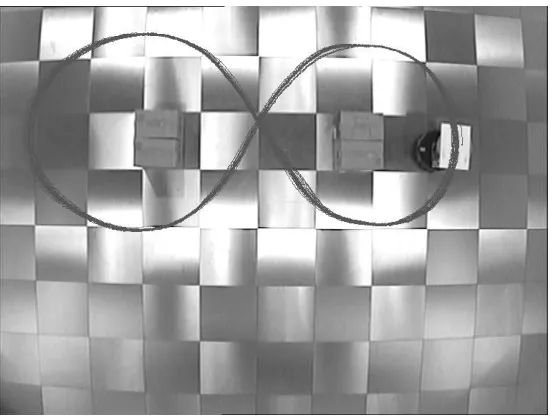
We applied our robot training strategy to program a reactive route following controller (figure 1). Although this route looks quite simple, it is actually quite difficult to learn due to the lack of landmarks in the environment. The sensor readings when the robot is in the middle of the route (labelled A in figure 1) are very similar but half of the time the robot has to turn right, while the other half it has to turn left. In order to learn this route a Magellan Pro Robot was first steered for 1 hour along the desired route by a human operator (fig-ure 1,left). During this stage sensor perceptions (fig(fig-ure 2), position, transitional and rotational velocities were recorded every 250 ms.

Figure 1: Left: Robot trajectory under manual control, used to obtain training data. Right: Trajectory taken under control of the obtained model given in table 1.

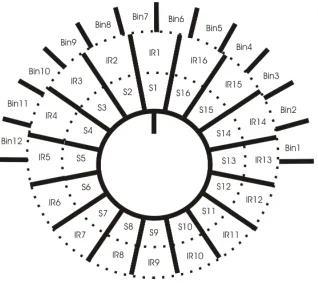
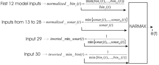
Having logged speeds and perceptions, we identified the robot’s movement using the NARMAX process, taking all sonar and laser measurements as inputs to the modelling process (figure 3). Laser ranges were averaged in twelve sec-tors of 15 degrees each (laser bins), resulting in a twelve-dimensional vector of laser-distances. Both laser bins and the 16 sonar sensor values were inverted and normalised, so that large readings indicate close-by objects. The resulting NARMAX model is shown in table 1. The model was then used to control the robot directly (figure 1, right).

Figure 3: Inputs used to model robot’s behaviour in the route shown in figure 1.

4

Behaviour Refinement through off-line Model

Analysis

Robot-environment interaction is strongly influenced by the environment in which the robot operates, and it is a common occurrence in mobile robotics that control code ceases to function correctly once the environment changes. To investigate the susceptibility of our Narmax model to such changes, we modi-fied the environment (by introducing or removing boxes, laddersetc.) until the model was no longer able to control the robot correctly.

Instead of trying to “guess” what was wrong, we decided to analyse the models to see the reasons behind the undesired behaviour, carrying out two different analyses: i) we computed the sensitivity of our control model with respect to each one of the inputs to see which inputs are the most relevant for the robot-behaviour, and ii) we used the partial derivatives of our model with respect to the identified most relevant inputs to analyse the stability of the model.

4.1

Sensitivity Analysis

˙

θ(t) = +0.08−0.50∗I1−0.62∗I4+ 0.46∗I6

+0.07∗I7₋0.09_∗I8+ 0.14_∗I9+ 0.02_∗I10

+0.20∗I12₋0.88_∗I13+ 0.22_∗I15₋0.04_∗I17

+0._004∗I18₋0.04_∗I19+ 0.20_∗I22 −0.02∗I26+ 0.11_∗I28₋0.43_∗I30

+0.041∗I2

1+ 0.02∗I 2

2−0.06∗I 2 3

+0.53∗I42−0.44∗I 2

6+ 0.01∗I 2 9 −8.70∗I302 −0.07∗I1_∗I2

+0._07∗I1_∗I3+ 0.44_∗I1_∗I4

+0.40∗I1∗I10−0.24∗I1∗I11

+0.83∗I1_∗I13+ 0.09_∗I1_∗I16 −0.79∗I1_∗I23₋0.04_∗I1_∗I25

+0._08∗I1_∗I29+ 3.58_∗I1_∗I30

+0._36∗I2_∗I4₋0.73_∗I2_∗I9 −0.05∗I2∗I12+ 0.04∗I2∗I25

+0.63∗I3_∗I8₋0.28_∗I3_∗I12

+0.11∗I3_∗I15₋0.48_∗I4_∗I10 −0.27∗I5_∗I8+ 0.11_∗I5_∗I13

+0._26∗I6_∗I8+ 0.02_∗I7_∗I17

+0._15∗I7_∗I18₋0.18_∗I7_∗I24 −0.17∗I8_∗I10+ 0.03_∗I8_∗I17 −0.10∗I10_∗I22+ 0.05_∗I10_∗I24

+0._03∗I12_∗I22+ 0.06_∗I12_∗I23

+0._01∗I12_∗I28+ 2.68_∗I13_∗I18 −0.30∗I13_∗I23₋1.99_∗I14_∗I18

+3.91∗I14_∗I30+ 0.13_∗I15_∗I17 −1.27∗I15_∗I18₋1.85_∗I15_∗I30

+0.05∗I16_∗I23₋0.13_∗I16_∗I29 −0.23∗I18_∗I22+ 0.89_∗I18_∗I23

+0._08∗I27_∗I28+ 5.06_∗I28_∗I29

Table 1: NARMAX model of the angular velocity θ˙ for the route following behaviour shown in figure 1. I1. . . I30, are the model

in-puts: the normalised laser bins, normalised sonar, inverted mini-mum sonar and laser readings, shown in figures 2 and 3.

4.1.1 Partial Derivative Analysis

Using Taylor’s theorem [Apostol, 1974], it is possible to estimate the change in the angular velocity of the robot due to changes in input sensor readings (eq 1).

∆ ˙θ=Pn

i=1 ∂ ˙ θ ∂Ii∆Ii+

1 2!

Pn

j=1

Pn

i=1 ∂

2_˙

θ

∂Ij∂Ii∆Ij∆Ii+

+_3!1 Pn

k=1

Pn

j=1

Pn

i=1 ∂

3_˙

θ

∂Ik∂Ij∂Ii∆Ik∆Ij∆Ii+. . . ,

(1)

where ˙θis the turning speed of the robot,nthe number of input signals in the model (30 in our case) andIiandIjrepresent model inputs 1. . .n(figure 3).

Figure 4: First full traversal of the desired route, taking 130 sec-onds total travelling time.

˙

θt+1≈θ˙t+ 30

X

i=1

∂θ˙ ∂Ii

∆Ii. (2)

Using equation 2, we can estimate the influence of each model input upon the robot’s steering speed. To estimate these influence values, we computed for every model-input the difference between the angular velocity ˙θt and the

predicted angular velocity when the input under consideration is removed from equation 2. Figure 5 shows the average influence of each model input for the first full traversal of the route (figure 4). The most relevant inputs turn out to beI13,I14,I15,I23,I28,I29 andI30.

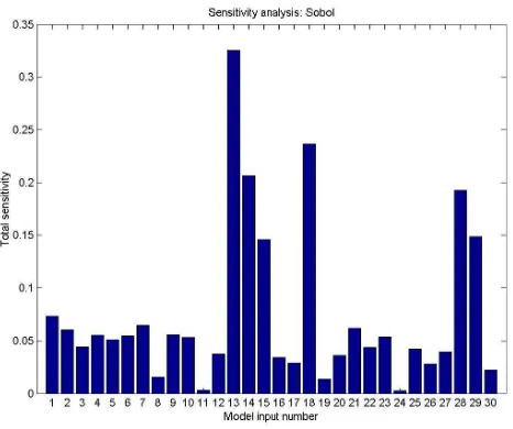
4.1.2 Sensitivity Analysis: Sobol Indices

We also applied the mechanism proposed by I. M. Sobol [Sobol, 1993] [Saltelli, 2002] to estimate the sensitivity of the model shown in table 1 with respect to each of its inputs. This analysis determines which input parameters contribute most to the model output, and which parameters are insignificant and might therefore be eliminated from the model.

We assume that a mathematical model is described by y = f(~x), where ~x represents a vector of n independent random variables defined in a unit n -dimensional cube. We’ll also assume that the joint probability density function of the input isp(x1, x2, ..., xn) =Q_in=1pi(xi). The total sensitivity off(~x) with

respect to each one of the different variablesxi, is calculated as the percentage

of the total variance off(~x) which is due to the variance inxi.

Figure 6 shows the sensitivities computed for each model input. I13, I14,

Figure 5: Average influence (estimated through partial derivatives) of each model-input.

conclusions we drew before from the partial derivative analysis (compare figure 6 with figure 5).

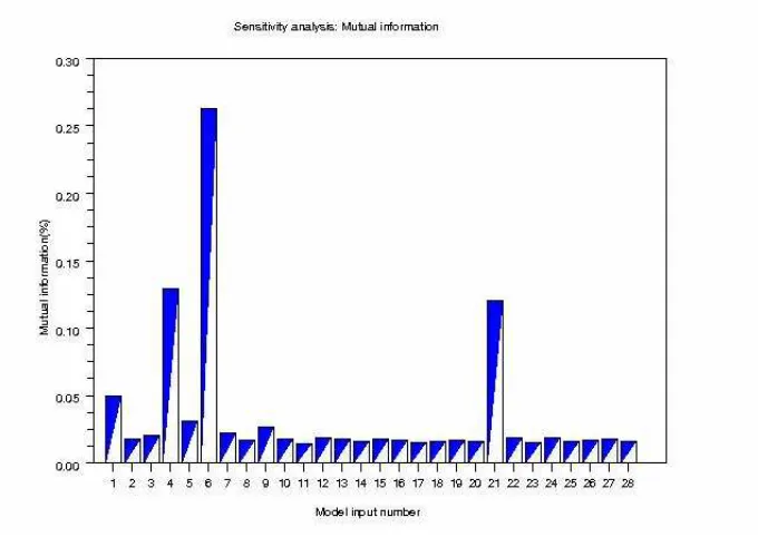
4.1.3 Mutual Information in Sensitivity Analysis

Finally, we estimated the sensitivity of the model with respect to each input by using the mutual informationIm between model inputuand model output y,

given in equation 3.

Im=H(u) +H(y)−H(u, y), (3)

withH(m) =−P

kp(mk)ln p(mk) and

H(m, n) =−P

k,lp(mk, nl)ln p(mk, nl). p(mk) is the probability that the value

of variablemfalls into bin k, and p(mk, nl) is the probability that variablem

falls into binkand variablenfalls into binl.

Using a Monte Carlo simulation, we estimate the sensitivity of the model with respect to inputui by generating a large number of random input vectors

~u, where only component ui is kept constant, and computing the mutual

in-formation between inputui and outputy. As the mutual information can be

interpreted as a measure of how much informationycontains aboutui, it will be

particularly high for componentsui that influence the model outputystrongly

(in other words, inputsui that are “important”).

Figure 7 gives the results, inputs I13,I14,I15, I18, I28, andI29 turn out to

be the most relevant — a good agreement with the results obtained in figures 5 and 6.

4.2

Stability Analysis

The last aspect we analysed is how much the angular velocity of the robot would change if one of the relevant sensors became noisy or if there were changes in the environment: we calculated partial derivatives of the angular velocity model with respect to the most relevant model inputs along the robot’s trajectory.

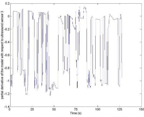
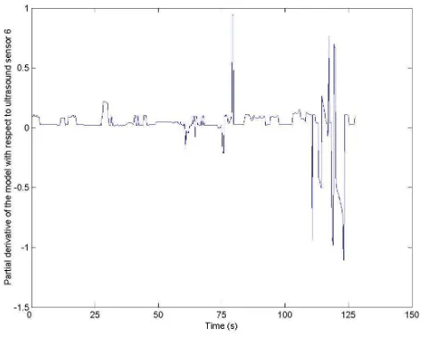
Figures 8 and 9 show the values of the partial derivatives of the model with respect to inputsI15 and I18 (sonar sensor 3 and 6, respectively). As we can

see, the partial derivative with respect to the third ultrasound sensor is quite often high during the first lap of the robot in the environment; this means that if any obstacle is placed at the left side of the robot when it is turning to the right (region A in figure 4), the robot-behaviour might be affected.

Figure 8: Value of the partial derivative of the control model with respect to input 15 (sonar 3) during the first lap of the robot in the environment shown in figure 4.

Regarding sonar 6 (figure 9), noisy readings would not be critical during most of the trajectory. If we consider figure 9 and the time it takes the robot to reach every part of the route (figure 4), we can see that the partial derivative is only high when the robot is between the two boxes in the environment. This is in good agreement with the results shown in figure 5.

If we now consider sonar 16 (model input I28), if a box was placed at, say,

location B (figure 4), the analysis given in figure 10 shows that that would affect the robot’s steering speed considerably — there are numerous high values of ∂Θ˙

∂I28

Figure 9: Value of the partial derivative of the model with respect to input 18 (sonar 6) during the first lap of the robot in the environment shown in figure 4.

5

Refining the Narmax Control Model

The analysis in section 4.2 revealed that the model is affected by fluctuations especially on sonars 3 and 16. We therefore decided to obtain a refined Narmax model, whose inputs are “myopic” sensor readings that are deliberately set to zero when they detect obstacles more than 2 m away. The model inputsIi we

used are given in equation 4

Ii =

(

δi·_bin2.0_(i) 0≤i≤12

δi·sonar2.0(i) 12≤i≤28,

(4)

with

δi=

1 ifbin(i)<2.0 orsonar(i)<2.0 0 otherwise

Figure 10: Value of the partial derivative of the model with respect to sonar 16 along the first lap of the robot in the environment shown in figure 4.

6

Sensitivity Analysis using Mutual Information

We have applied three different strategies to carry out a sensitivity analysis, and consider mutual information to be the best amongst them, due to its low computational cost and intuitive meaning: It measures the information ob-tained about a particular model input, given a particular model output. If the model output,y, is completely independent of a particular model input,u, then H(u, y) =H(u) +H(y) and, therefore, Im = 0. To demonstrate the utility of

mutual information in sensitivity analysis, we will apply it to further models in this section.

6.1

Door traversal behaviour

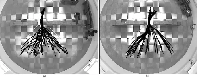
We have first considered a model that identifies the behaviour of a manually driven robot across the door shown in figure 12. The model is given in table 2.

Figure 12: a) Robot trajectories under manual control (39 runs, training data). b) Trajectories taken under model control (41 runs, test data). The white lines on the floor were used to aid the human operator in selecting start locations, they were invisible to the robot.

Table 2: NARMAX model of the steering direction and velocityθ˙of the robot for the door traversal behaviour. The sonar readings are represented ass1,· · ·, s16, and the 12 laser bins ared1,· · ·, d12.

˙

θ(t) = 0.272 + 0.142∗(1/d1(t))−0.470∗(1/d3(t))

−0.070∗(1/d4(t))−0.347∗(1/d6(t)) + 0.157∗(1/d8(t))

+0.091∗(1/d9(t))−1.070∗(1/s9(t))−0.115∗(1/s12(t))

+0.130∗(1/d3(t))2−0.166∗(1/d8(t))2+ 0.183∗(1/s9(t))2

+0.081∗(1/(d1(t)∗d3(t)))−0.098∗(1/(d1(t)∗d4(t)))

−0.382∗(1/(d1(t)∗d5(t)))−0.204∗(1/(d1(t)∗d6(t)))

−0.049∗(1/(d1(t)∗d8(t)))−0.078∗(1/(d1(t)∗s8(t)))

+0.060∗(1/(d2(t)∗s7(t))) + 0.300∗(1/(d3(t)∗d5(t)))

+0.037∗(1/(d3(t)∗s5(t))) + 0.209∗(1/(d3(t)∗s12))

+1.014∗(1/(d4(t)∗d6(t))) + 0.061∗(1/(d4(t)∗s4(t)))

+0.273∗(1/(d4(t)∗s12(t)))−0.536∗(1/(d5(t)∗d6(t)))

+0.230∗(1/(d5(t)∗d7(t)))−0.503∗(1/(d6(t)∗d9(t)))

+2.516∗_(1/(d6(t)∗_s9(t)))−_0.067∗_(1/(d6(t)∗_s13(t))) −_0.009∗_(1/(d7(t)∗_{s15(t))) + 0.086}∗_(1/(d8(t)∗_s3(t))) −0.038∗(1/(d8(t)∗s6(t)))−0.060∗(1/(d9(t)∗s4(t)))

−0.067∗(1/(d10(t)∗d12(t)))−0.040∗(1/(d10(t)∗s12(t)))

+0.059∗(1/(d11(t)∗s1(t)))−0.045∗(1/(d12(t)∗s7(t)))

6.2

Wall following behaviour

The second robot’s behaviour that we have analysed using mutual information was a wall following behaviour [Kyriacou et al., 2005]. In this case, instead of using the robot-training strategy described in the introduction, an artificial neural network (ANN) based controller was used to drive the robot first, its motion was then identified using the Narmax model shown in table 3. The ANN-based controller [Iglesias et al., 1998] uses a set of self-organising maps (SOM) [Kohonen, 1997] and a multilayer perceptron (MLP) neural network to process the information provided by 9 ultrasound sensors and thus determine the angular velocity the robot should attain at each instant, figure 14.

Figure 14: Diagrammatic representation of the ANN wall-following program used to initially control the movement of the robot. This controller uses the readings coming from the ultrasound sensors 1,2,3,16,15,14,13,12 and 11 (figure 2).

ωmodel(t) =₋0.282₋0.129_∗(1/s1(t)) −0.039∗(1/s1(t₋1))₋0.076_∗(1/s1(t₋2)) −0.017∗(1/s3(t)) + 0.007_∗(1/s5(t))

+0.017∗(1/s9(t)) + 0.009_∗(1/s10(t)) −0.007∗(1/s12(t₋1)) + 0.165_∗(1/s13(t)) −0.019∗(1/s13(t₋1)) + 0.079_∗(1/s14(t)) −0.051∗(1/s15(t))₋0.072_∗(1/s16(t))

+0.134∗(1/(s1(t)) 2

) + 0.017∗(1/(s1(t₋1)) 2

) +0.096∗(1/(s1(t₋2))

2

) + 0.001∗(1/(s2(t)) 2

) +0.018∗(1/(s7(t₋2))

2

)−0.019∗(1/(s13(t)) 2

) +0.056∗(1/(s15(t))

2

) + 0.099∗(1/s16(t)) 2

+0.063∗(1/(s1(t₋1)_∗s16(t₋1)) −0.071∗(1/(s1(t₋2)_∗s9(t₋2))

+0.039∗(1/(s2(t)_∗s14(t))) −0.038∗(1/(s2(t₋1)_∗s6(t)

+0.059∗(1/(s3(t₋1)_∗s15(t)))

+0.003∗(1/(s13(t)_∗s13(t₋1))) −0.027∗(1/(s13(t)_∗s14(t)))

Table 3: The NARMAX model of the ANN wall-following task, showing the rotational velocityω as a function of the sonar sensor valuessi,∀i= 1, ...,16.

7

Conclusions

Robot training using system identification is a novel method of obtaining robot control code that eliminates the need for iterative refinement of code through trial and error. To achieve sensor-motor tasks we first operate the robot under human supervision, logging sensor motor information at the same time. We then use the Narmax modelling approach to obtain a control model which identifies the coupling between sensor perception and motor responses, which is used to control the robot to move autonomously.

In this paper we show how the mathematical analysis of these models can be used to formulate hypotheses that allow the post-hoc modification of models. We demonstrate how sensitivity analysis can be used to determine the most relevant sensors in the robot’s behaviour, so that a subsequent stability analysis of those relevant sensors — through partial derivatives — pinpoint those regions in the environment where sensor accuracy is crucial.

We used three different methods of sensitivity analysis, and in conclusion argue that mutual information is the most suitable indicator of sensor relevance, because it computes how much information an output conveys about a particular input — it has an actual, physically grounded meaning.

Acknowledgements

The RobotMODIC project is supported by the British Engineering and Physical Sci-ences Research Council under grant GR/S30955/01. Roberto Iglesias is supported through Spanish research grants PGIDIT04TIC206011PR, TIC2003-09400-C04-03 and TIN2005-03844.

We thank Theo Kyriacou and Otar Akanyeti for their help in some of these exper-iments, and their helpful comments on this work.

References

[Analytical and Cognitive Robotics Group, 2007] Analytical and Cognitive Robotics Group (2007). http://cswww.essex.ac.uk/staff/udfn/robotmodic/.

University of Essex.

[Apostol, 1974] Apostol, T. (1974). Mathematical Analysis. Addison-Wesley Publishing Company.

[Chen and Billings, 1989] Chen, S. and Billings, S. (1989). Representations of non-linear systems: The narmax model. International Journal of Control, 49:1013–1032.

[Eykhoff, 1981] Eykhoff, P. (1981). Trends and Progress in System Identifica-tion. Pergamon Press.

[Iglesias et al., 2006] Iglesias, R., Nehmzow, U., Kyriacou, T., and Billings, S. (2006). Current Topics in Artificial Intelligence. Lecture Notes in Artificial Intelligence, volume 4177, chapter Training and Analysis of Mobile Robot Behaviour Through System Identification. Springer.

[Iglesias et al., 1998] Iglesias, R., Regueiro, C. V., Correa, J., Schez, E., and Barro, S. (1998). Improving wall following behaviour in a mobile robot using reinforcement learning. In Proc. of the International ICSC Symposium on Engineering of Intelligent Systems. ICSC Academic Press.

[Kohonen, 1997] Kohonen, T. (1997). Self-Organizing Maps. Springer, second edition.

[Korenberg et al., 1988] Korenberg, M., Billings, S., Liu, Y. P., and McIlroy, P. J. (1988). Orthogonal parameter estimation algorithm for non-linear stochastic systems. International Journal of Control, 48:193–210.

[Kyriacou et al., 2006] Kyriacou, T., Akanyeti, O., Nehmzow, U., Iglesias, R., and Billings, S. (2006). Visual task identification using polynomial models. InProc. of Towards Autonomous Robotic Systems.

[Kyriacou et al., 2005] Kyriacou, T., Nemhzow, U., Iglesias, R., and Billings, S. A. (2005). Task characterisation and cross-platform programming through system identification. INT. J. ADVANCED ROBOTIC SYSTEMS, 2:317– 324.

[Nehmzow et al., 2006] Nehmzow, U., Iglesias, R., Kyriacou, T., and Billings, S. A. (2006). Robot learning through task identification. International Jour-nal on ROBOTICS AND AUTONOMOUS SYSTEMS.

[Saltelli, 2002] Saltelli, A. (2002). Making best use of model evaluations to compute sensitivity indices. Computer Physics Communications, 145.