Accurate robot simulation through system identification

This is a repository copy of Accurate robot simulation through system identification. White Rose Research Online URL for this paper:

http://eprints.whiterose.ac.uk/74625/

Monograph:

Kyriacou, T., Nehmzow, U., Inglesias, R. et al. (1 more author) (2008) Accurate robot simulation through system identification. Research Report. ACSE Research Report no. 968 . Automatic Control and Systems Engineering, University of Sheffield

Reuse

Unless indicated otherwise, fulltext items are protected by copyright with all rights reserved. The copyright exception in section 29 of the Copyright, Designs and Patents Act 1988 allows the making of a single copy solely for the purpose of non-commercial research or private study within the limits of fair dealing. The publisher or other rights-holder may allow further reproduction and re-use of this version - refer to the White Rose Research Online record for this item. Where records identify the publisher as the copyright holder, users can verify any specific terms of use on the publisher’s website.

Takedown

If you consider content in White Rose Research Online to be in breach of UK law, please notify us by

Accurate Robot Simulation through System Identification

T Kyriacou

, U Nehmzow

, R Inglesias

, S A Billings

~

School of Computing and Mathematics, University of Keele #Dept Computer Science, University of Essex

*Electronics and Computer Science, University of Santiago de Compostela, Spain

Department of Automatic Control and Systems Engineering

The University of Sheffield, Sheffield, S1 3JD, UK

Research Report No. 968

Accurate Robot Simulation

through System Identification

Theocharis Kyriacou

Ulrich Nehmzow

∗

_{Roberto Iglesias}

S. A. Billings

a_{School of Computing and Mathematics, Keele University, Keele ST5 5BG, UK}

b_{Department of Computing and Electronic Systems, University of Essex,}

Colchester CO4 3SQ, UK

c_{Department of Electronics and Computer Science, University of Santiago de}

Compostela, Spain.

d_{Department of Automatic Control and Systems Engineering, University of}

Sheffield, UK

Abstract

Robot simulators are useful tools for developing robot behaviours. They provide a fast and efficient means to test robot control code at the convenience of the office desk. In all but the simplest cases though, due to the complexities of the physical systems modelled in the simulator, there are considerable differences between the behaviour of the robot in the simulator and that in the real world environment.

In this paper we present a novel method to create a robot simulator using real sensor data. Logged sensor data is used to construct a mathematically explicit model (in the form of a NARMAX polynomial) of the robot’s environment. The advantage of such a transparent model — in contrast to opaque modelling methods such as artificial neural networks — is that it can be analysed to characterise the modelled system, using established mathematical methods

In this paper we compare the behaviour of the robot running a particular task in both the simulator and the real-world using qualitative and quantitative measures including statistical methods to investigate the faithfulness of the simulator.

1 Introduction

Fundamentally, the behaviour of a robot is influenced by three components: i) the robot’s hardware, ii) the program it is executing and iii) the environment it is operating in (see figure 1). This results in a highly complex, usually non-linear, system. A robot program written with a specific task in mind almost never produces the desired robot behaviour right from the beginning. This is because many idealistic assumptions are made as far as the the robot’s hard-ware and environment are concerned. Furthermore, even though the robot’s programming language provides a very precise means of dictating the task in mind, a reasonably complex program can never be tested fully and is likely to cause some unexpected behaviour at some point during its execution.

or Task Program Code Robot

Environment

Fig. 1.The behaviour of a robot emerges from the interaction between robot, task and environment.

The lack of a formal design methodology that is based on a theory of robot-environment interaction (which would allow the methodical design of mobile robot control programs) means that control programs have to be developed through an empirical trial-and-error process. This is costly, time-consuming and error prone. This problem is addressed in previous work under the Robot-MODIC project (see [1–3]).

The lack of a theoretical foundation for mobile robotics means that

develop-ment tools have to be based on assumptions (e.g.idealised, simplified models

of sensors, simplified environment modelsetc) that commonly result in

signif-icant discrepancies between predicted and actually observed behaviour of the physical mobile robot.

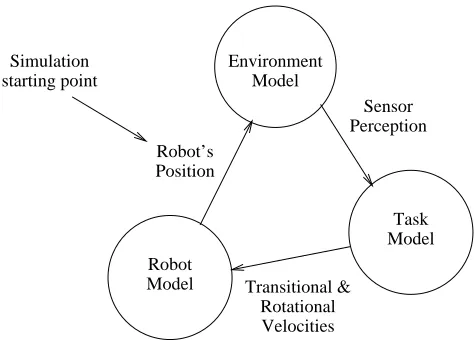
Environment Model

Sensor Perception

Task Model Robot

Model Transitional & Rotational Velocities Robot’s

Position Simulation

starting point

Fig. 2. A diagrammatic representation of the function of the robot simulator. Based on the robot’s position and orientation the environment model produces the estimated sensor perception. This is then passed to the task model which computes the transitional and rotational velocities of the robot. Finally the velocities are used by the robot model in order to compute the next position and orientation of the robot in the environment.

Robot simulators are convenient robotics research tools for developing and testing new robot controllers. One of their main advantages is that they save significant time and effort which is otherwise spent in working with real world experimental setups [4]. This is because: (i) time in simulation usually runs faster than real time and therefore the results of experiments are ready quicker and (ii) because less time is spent to setup an environment in simulation than in the real world.

In addition, simulations provide the only absolutely consistent method for experimental repetition. This is particularly helpful, for example, when we need to compare two robot controllers under identical conditions (robot and environment). Finally, with some learning paradigms such as reinforcement learning, it is necessary to allow the robot to err in order to learn. Simulating the robot, in such cases, would save any time required to reset the experimental setup after such errors and will also minimise any damage risk to the robot.

1.1 Mobile Robot Simulation

The advantages, then, of mobile robot simulation are obvious, and computer models of robot-environment interaction are clearly desirable as development tools. Consequently, large parts of the robotics research community have adopt-ed simulation as a viable and fundamental research tool, and a number of simulators, such as Player-Stage [5] and Webots [6], as well as those supplied with specific robot platforms[7–9], are widely used.

These general purpose robot simulators, as well as models of specific robots,

such as [10,11], have in common that they aim to begenerally applicable, i.e.

generic, and that they are therefore based on general assumptions about kine-matics and dynamics of the robot and environment properties. The Webots simulation, for instance, defines mass distribution matrices for robot compo-nents, friction coefficients, bounciness etc in order to achieve a certain degree of fidelity, a RoboCup simulation is similar[11]. Player-Stage aims for “good enough fidelity” [5], where “good enough” is not defined (see discussion in section 3.2.1). Some simulations use generic kinematics and dynamics mod-els as well as generic noise modmod-els, usually assuming all noise affecting robot operation is Gaussian [10].

Generic robot simulators, based on general assumptions about the robot and its environment, have attracted criticism in the past [12,13] that has, so far, only been addressed to a limited degree by the research community. As we argued in [14,15], and continue to believe, faithful simulation of robot-environment interaction has to be data-driven, and can therefore only model

specific experimental scenarios. In all but the simplest robotics experiments one finds that certain parts of the environment give rise to extreme percep-tions, for example through specular reflections off smooth surfaces — a phe-nomenon that a generic simulator can not model.

This paper therefore addresses the issue of faithful computer simulation of

robot-environment interaction, not generic simulation, and for this reason uses a modelling technique that is data-driven. Related work that is therefore much closer to our proposal here is the simulator built by Lund and Miglino [16], which stores logged data in a lookup table and uses interpolation for the prediction of sensory perception at unvisited locations, or the neural network-based simulator presented in [14,15], which trains a multilayer Perceptron to model the relationship between robot location and sensor perception. Both of these approaches result in highly accurate models that are able to predict sensory perceptions, even in areas having perceptual discontinuities.

Besides faithful simulation, there is, however, another motivation behind the

the relationship between location and perception. An opaque neural network model is unsuitable for this, and an interpolation method is, strictly speaking, not a modelling (i.e. generalising) approach at all.

In one sentence, we would like to obtain a faithful computer model of

robot-environment interaction that retains, in simplified form, the essence of that

interaction, and that is transparent and therefore amenable to analysis. We

achieve these three objectives using system identification[17].

Compared with other modelling approaches, such as artificial neural networks or lookup tables, system identification offers noticeable benefits:

• The obtained models are extremely compact, consisting of one polynomial

of typically a few dozen terms.

• The models are transparent, and therefore analysable by standard

tech-niques such as sensitivity analysis. Examples of such analyses are given in [18] and [19].

1.2 The NARMAX modelling procedure

The NARMAX modelling approach is a parameter estimation methodology for identifying the important model terms and associated parameters of unknown nonlinear dynamic systems. For multiple input, single output noiseless systems this model takes the form:

y(n) =f(u1(n), u1(n−1), u1(n−2),· · ·, u1(n−Nu),

u1(n)2, u1(n−1)2, u1(n−2)2,· · ·, u1(n−Nu)2, · · ·,

u1(n)l, u1(n−1)l, u1(n−2)l,· · ·, u1(n−Nu)l,

u2(n), u2(n−1), u2(n−2),· · ·, u2(n−Nu),

u2(n)2, u2(n−1)2, u2(n−2)2,· · ·, u2(n−Nu)2, · · ·,

u2(n)l, u2(n−1)l, u2(n−2)l,· · ·, u2(n−Nu)l, · · ·,

ud(n), ud(n−1), ud(n−2),· · ·, ud(n−Nu),

ud(n)2, ud(n−1)2, ud(n−2)2,· · ·, ud(n−Nu)2, · · ·,

ud(n)l, ud(n−1)l, ud(n−2)l,· · ·, ud(n−Nu)l,

y(n−1), y(n−2),· · ·, y(n−Ny),

y(n−1)l_{, y(n−2)}l_{,· · ·, y(n−N} y)l)

were y(n) and u(n) are the sampled output and input signals at time n

re-spectively, Ny and Nu are the regression orders of the output and input

re-spectively and d is the input dimension. f() is a non-linear function, this is

typically taken to be a polynomial or wavelet multi-resolution expansion of

the arguments. The degree l of the polynomial is the highest sum of powers

in any of its terms.

Noise is always present in physical systems and can be accommodated as part of the NARMAX model. In the present study we have initially assumed that the effects of the noise are small and can be neglected. In later studies the effects of any noise will be accommodated by fitting noise models as part of the identification procedure to ensure that unbiased models are obtained.

The NARMAX methodology breaks the modelling problem into the following steps:

(1) Structure detection, (2) Parameter estimation, (3) Model validation, (4) Prediction and (5) Analysis.

These steps form an estimation toolkit that allows the user to build a con-cise mathematical description of the system. These procedures are now well established and have been used in many modelling domains [20].

A detailed procedure of how structure detection, parameter estimation and model validation is done is presented in [21]. A brief explanation of these steps is given below.

Any data set that we intend to model is first split in two sets (usually of equal

size). We call the first the estimation data set and it is used to determine

the model structure and parameters. The remaining data set is called the

validation data set and it is used to validate the model.

The initial structure of the NARMAX polynomial is determined by the

in-puts u, the output y, the input and output orders N_u and N_y respectively

and the degree l of the polynomial. Any signal that influences the output

the estimated NARMAX model will indicate any insignificant or redundant inputs.

Before any removal of model terms an equivalentauxiliary model is computed

from the original NARMAX model. The model terms of the auxiliary model are orthogonal. This allows the computation of their associated parameters to be done in a sequential manner which is computationally more efficient.

The calculation of the auxiliary model parameters and the refinement of the model’s structure is an iterative process which allows the model to be built up one term at a time. This is followed by model validation.

After the model validation step, if there is no significant error between the model-predicted output and the actual output, non-contributing model terms are removed in order to reduce the size of the polynomial as much as possible. This is primarily done to increase the speed of computation of the model output during its use and also to avoid over-fitting the model to the training data.

To determine the contribution of a model term to the output the Error Re-duction Ratio (ERR) [21] is computed for each term. The ERR of a term is the percentage reduction in the total mean-squared error (i.e. the difference between model-predicted and true system output) as a result of including (in the model equation) the term under consideration. The bigger the ERR is, the more significant the term. Model terms with ERR under a certain threshold (usually around 0.05%) are removed from the model polynomial in the last step of each iteration during the refinement process.

In the following iteration, if the error is higher as a result of the last removal of model terms then these are re-inserted back into the model equation and the model is considered as final. Finally, the NARMAX model parameters are computed from the auxiliary model.

2 Experimental methods

2.1 Experimental setup

The robot used in our experiments is the Magellan Pro autonomous mobile

robotRadix (figure 3). The robot is equipped with 16 sonar, 16 infra-red and

16 tactile sensors distributed uniformly around its circumference. A SICK

laser range finder is also present which scans the front semi-circle of the robot

([0◦

,180◦

]) with a radial resolution of 1◦

and a distance resolution of less than 1 centimetre. The robot also incorporates a video camera. In the work presented in this paper primarily the laser sensor is used.

Fig. 3. Radix, the Magellan Pro mobile robot used in the experiments described in this paper. The visual target visible on the top of the robot was used for vision-based trajectory tracking.

During experiments withRadix, the input from all its sensors (apart from the

tracking system are aligned using time as the common reference. Finally, due to the high sampling rate used, it is often necessary to subsample the collected data before it is used for modelling and analysis.

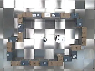
Experimental setups of the robot’s static environment are built in a dedicated robot arena usually using carton boxes. An example of one such experimental setup is shown in figure 4.

Fig. 4.Bird’s eye view of an experimental setup. The longest width and height of the environment is 3.9 and 2.4 metres respectively. The image is taken with the overhead camera used for tracking the position of the robot.

To build the simulator,Radix is first used to collect data from the environment

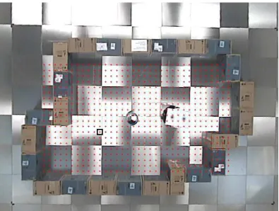
that needs to be modelled. This is done using an exploratory task in order to scan the environment using the robot’s sensors as thoroughly as possible. Figure 5 shows the trajectory of the robot during one such exploration session.

2.2 Environment modelling

2.2.1 Method 1: Continuous Model building

Fig. 5.The trajectory of the robot during an exploration of the environment. The task that was being executed was an obstacle avoidance task using the robot’s laser sensor. To produce the shown trajectory, the robot moved in the environment for approximately 2 hours.

orientation in the environment. This is the basis of our robot simulator.

The environment model MCS M

is comprised of a set of functions, each of which is itself a model of the environment but only as perceived by the robot when it is at a particular location:

MCS M

={Smp_{} (1)}

S_(xmpm,yn)=f(ϕ) (2)

m= 1, ..., w n= 1, ..., h ϕ∈[−π,+π]

where S_(xmpm,yn) is the model-predicted sensor perception when the robot is

at location (xm, yn). This is a function of the angle ϕ in which the particular

sensor is facing. We shall, from now on, callS_(xmpm,yn) themodel-predicted sensor

signature of location (xm, yn). The set of locations {(x, y)} are chosen to be

Fig. 6. A 10 cm grid superimposed on the image of the environment. Location (1.78, 2.31) is shown in black, the laser perception of the robot at this location is given in figure 7.

the surface area of the environment to be modelled. As an example, the grid locations of a 10 cm spaced grid for the environment shown in figure 4 are shown in figure 6.

Each sensor signature, perceived at a particular grid location, is then modelled using a NARMAX polynomial, using real sensor data obtained during the

exploration of the environment. This approximated sensor signature{Sa

(xm,yn)}

for location (xg

m, yng), represented by a non-linear polynomial, contains two

elements: the sensor angle ϕ and the approximated range value of the sensor

vϕ corresponding to this angle:

Sa

(xm,yn)={(ϕ, vϕ)} (3)

ϕ∈[−π,+π]

The sensor range value is approximated because it is taken to be the same as

that of the nearest value available in the exploration data (i.e. the same as

Laser sensor range (metres)

Laser sensor angle (rad)

0 1 2 3 4 5 6 7

0.5 1.0 1.5 2.0 2.5 3.0

Fig. 7.The laser sensor signature at grid location (1.78, 2.31) metres. The sensor values are shown starting from 0 radians (east direction with respect to figure 6) clockwise to

2π radians.

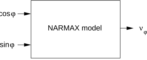
sinϕ cos ϕ

NARMAX model ν_ϕ

Fig. 8.Inputs and output of the NARMAX model for each sensor signature in the grid of locations chosen to model the environment, were ϕ is the sensor angle and vϕ the

approximated range value perceived by the sensor at this angle.

The resolution of the angleϕ isπ/180 rad thus makingSa _{a signature of 360}

samples. Figure 7 shows the approximated signature of the laser sensor at grid location (1.78, 2.31) metres (shown as a black square in figure 6).

After obtaining each approximated grid signature (Sa_{), the NARMAX}

mod-elling methodology is used to estimate the continuous function (Smp_{) that}

rep-resents Sa_{. To avoid the discontinuity at ϕ = ±π, we use sin(ϕ) and cos(ϕ)}

as inputs to the model, rather thanϕ directly. The output of the model is the

sensor range value ν (see figure 8).

were used (i.e. l = 5, Nu = 0, Ny = 0). For the signature shown in figure 7

the following polynomial was obtained:

S_(1.78,2.31)mp = (4)

+1.489

−1.625∗u1 −0.766∗u2 −0.602∗u2₁

+4.726∗u3₁

+1.258∗u3₂

+0.379∗u4₁

−2.860∗u5 1

+0.329∗u1∗u2(n)

−0.164∗u1∗u2(ϕ)3

+1.178∗u2∗u1(ϕ)4

where

u1=sin(ϕ)

u2=cos(ϕ)

ϕ∈[−π,+π]

Following the example of the grid location (1.78, 2.31) the model-predicted laser signature values at this location produced by evaluating the function

above for values ofϕ in the range [−π,+π] is shown in figure 9. The

approxi-mated sensor signature at location (1.78, 2.31) is also shown for comparison.

In a similar way, the complete environment model is composed by finding the models corresponding to each approximated grid signature. Note that the degree of the model polynomials (here degree 5) is adaptive and is decided based on how well the model fits the experimental data. This can be bigger or smaller depending on the complexity of the sensor signature which is related to the complexity of the environment topology.

Laser sensor range (metres)

Laser sensor angle (rad)

0 1 2 3 4 5 6 7

0.5 1.0 1.5 2.0 2.5 3.0

Fig. 9. Approximated (thin line) and model-predicted (thick line) sensor signature at location (1.78, 2.31) metres.

2.2.2 Model validation

In order to validate the environment models obtained by the method described thus far, test data is collected in the real environment while the robot

exe-cutes a new, different task in the laboratory (the validation task) right after

the exploratory phase. The validation task is also executed in the robot simu-lator and the two obtained trajectories are compared. A complete example of environment modelling and validation is presented in section 3.

2.2.3 Method 2: Piecewise signature modelling

We implemented an alternative to the above method that improves the pre-diction accuracy of the environment model considerably by modelling smaller segments of each grid signature rather than the entire signature. Here, each

grid signature is modelled using a set of NARMAX polynomial functions

in-stead of only one. We call this the piecewise signature modelling method.

with the previous surface or at a different distance (see figure 10).

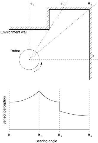
θ₃ θ₂

θ₁ θ₄

θ₁ θ₂ θ₃ θ₄

Sensor perception

Bearing angle Robot

Environment wall

Fig. 10.Two occasions where cusps appear in the sensor signature. As the robot rotates anti-clockwise at the same location one laser sensor scans the wall surface from ϕ₁ to

ϕ4. Two cusps appear in the signature recorded: the first at ϕ2 and the other at ϕ3.

Actually in the latter case two cusps exist, one on top of the other.

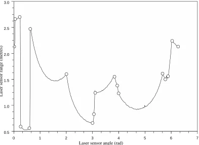
Figure 11 shows the location of the cusps of the laser sensor signature shown in figure 7.

The complete environment model MP S M

Laser sensor range (metres)

Laser sensor angle (rad)

0 1 2 3 4 5 6 7

0.5 1.0 1.5 2.0 2.5 3.0

Fig. 11. The circles indicate the location of the cusps. These are determined from the magnitude of the second derivative of the sensor signature.

MP S M

={Smp_{} (5)}

S_(xmpm,yn)={f

i_{(ϕ), ϕ}

i 6ϕ < ϕi+1} (6)

m= 1, ..., w n= 1, ..., h i= 1, ..., k ϕ∈[−π,+π]

where S_(xmpm,yn) is now a set of k polynomials each of which models a segment

of the approximated sensor signature at grid location (xm, yn).

As an example, the piecewise model of the signature shown in figure 11 is given in table 1, figure 12 shows the piecewise model-predicted sensor signature and the approximated signature.

where

u1=sin(ϕ)

S_(1.78,2.31)mp =                                                                                                             

+2.130 , ϕ= 0.000

+2.065 + 15.186∗u1 , 0.000< ϕ <0.035

+5.349−0.042∗u1−2.695∗u2 , 0.0356ϕ <0.209

+15.945−61.998∗u1 , 0.2096ϕ <0.244

+4.063−1.482∗u1−3.210∗u2 , 0.2446ϕ <0.576

−35.633 + 65.876∗u1 , 0.5766ϕ <0.611

+3.772−2.336∗u1−0.051∗u2 , 0.6116ϕ <1.990

+3.203−0.793∗u1+ 2.404∗u2 , 1.9906ϕ <2.985

+1.138−3.238∗u1 , 2.9856ϕ <3.037

+1.772−8.793∗u1 , 3.0376ϕ <3.089

+2.719−0.005∗u1+ 1.471∗u2 , 3.0896ϕ <3.822

+2.953 + 2.233∗u1 , 3.8226ϕ <3.927

+4.624 + 4.580∗u1 , 3.9276ϕ <3.979

+2.283 + 1.375∗u1+ 0.043∗u2 , 3.9796ϕ <5.655

+0.890−1.220∗u1 , 5.6556ϕ <5.760

+1.747 + 0.481∗u1 , 5.7606ϕ <5.864

+7.620 + 6.408∗u1−3.803∗u2 , 5.8646ϕ <6.021

+3.546−0.265∗u1−1.426∗u2 , 6.0216ϕ <6.266

+2.130 , ϕ= 6.266

(7)

Table 1

Piecewise model of the sensor signature shown in figure 11

In simulation, the environment model obtained using the piecewise approach is used to obtain the robot’s sensor perception in a similar fashion as with

model MCS M

but in this case there is an additional step: The bearing of the sensor whose value is sought determines which polynomial function of the signature must be used. In the example given above (equation 7), if the robot

in simulation is nearest to location (1.78,2.31) metres so that model S_(1.78,2.31)mp

is selected and, say, a single laser sensor component is facing 0.75 rad, then the polynomial

S_(1.78,2.31)mp |ϕ=0.75= +3.772−2.336∗u1−0.051∗u2

would be used to obtain the model-predicted perception of that laser sensor component (in this case 2.14 metres).

Laser sensor range (metres)

Laser sensor angle (rad)

0 1 2 3 4 5 6 7

0.5 1.0 1.5 2.0 2.5 3.0

Fig. 12. Approximated (dark-coloured line) and model-predicted (light-coloured line), using the piecewise modelling method, sensor signature at location (1.78, 2.31) metres.

example using both modelling approaches explained above. Both models ob-tained are tested by comparing the robot’s behaviour in a simulator and that in the real world for the same robot task.

3 Experimental results

The environment shown in figure 4 was modelled using the two methods de-scribed in the previous section. Only the laser sensor was modelled in the following example.

Initially the robot was allowed to execute an exploratory task using its laser sensor. This was essentially an obstacle avoidance task. The aim was to cause the robot to visit the entire environment as thoroughly as possible in order to record, through its sensors, all features in the environment. The trajec-tory of the robot after executing the exploratrajec-tory task in the environment for approximately 2 hours is shown in figure 5.

The grid locations whose signatures are approximated using sensor data from

the exploration phase are shown in figure 6. The grid spacing in bothx and y

Using the two modelling methods described in section 2.2, two models of the environment were obtained: first, by modelling the entire approximated

laser sensor signature of each grid location using one NARMAX polynomial

(Complete Signature Model MCS M

, see section 2.2); second, by modelling

the approximated laser sensor signature of each grid location using multiple

NARMAX polynomials (Piecewise Signature ModelMP S M

, see section 2.2.3).

ModelMCS M

resulted in a set of 680 polynomials (one for each grid location),

modelMP S M

in a set of 14280 polynomials (i.e. an average of 21 polynomials for each grid location).

In order to evaluate each model, the behaviour of the robot while running a particular, new task in the simulated environment (using either of the models) was compared with that of the real robot executing the same task in the real environment. This test data was obtained in the environment that had been modelled during the initial exploration shown in figure 5. The test control program was a wall-following task using the robot’s laser sensor. The trajec-tory of the robot during the collection of the test data is shown in figure 13. The same wall-following task was then implemented in a simulator using, first,

model MCS M

and then model MP S M

.

Fig. 13. The trajectory of the robot during the execution of the wall-following task in the environment.

Figures 14 and 15 show the trajectory of the robot in simulation (using models

MCS M

and MP S M

world (used as the “ground truth”) when executing the wall-following task.

y odometry (metres)

x odometry (metres)

0.5 1.0 1.5 2.0 2.5 3.0 3.5 4.0 4.5 −3.0

−2.8 −2.6 −2.4 −2.2 −2.0 −1.8 −1.6 −1.4 −1.2

Fig. 14. The trajectory of the robot in the simulator using environment modelMCS M

(light-coloured line). This is the environment model which usesone NARMAX polyno-mial for each grid location. The robot’s trajectory obtained during the collection of the test data (ground truth) is also shown (dark-coloured line) for comparison.

y odometry (metres)

x odometry (metres)

0.5 1.0 1.5 2.0 2.5 3.0 3.5 4.0 4.5 −3.0

−2.8 −2.6 −2.4 −2.2 −2.0 −1.8 −1.6 −1.4 −1.2

Fig. 15. The light-coloured line shows the trajectory of the robot in the simulator using environment modelMP S M

(piecewise signature model). This is the environment model which uses several NARMAX polynomial for each grid location. The robot’s trajectory obtained during the collection of the test data (ground truth) is also shown (dark-coloured line) for comparison.

location to determine the robot’s sensor perception. The trajectory of the simulated robot during this run is shown in figure 16.

y odometry (metres)

x odometry (metres)

0.5 1.0 1.5 2.0 2.5 3.0 3.5 4.0 4.5 −3.0

−2.8 −2.6 −2.4 −2.2 −2.0 −1.8 −1.6 −1.4 −1.2

Fig. 16.The trajectory of the robot in the simulator using sensor data directly from the approximated grid signatures (look-up table model) to determine the sensor perception of the simulated robot (light-coloured line). The robot’s trajectory obtained during the collection of the test data (ground truth) is also shown (dark-coloured line) for comparison.

To assess the faithfulness of each of the three models obtained we conducted a qualitative and a quantitative comparison between the pairs of trajectories presented in figures 14, 15 and 16, which is discussed in the following section.

3.1 Qualitative assessment of experimental results

Visual comparisons between figures 14 and 15 show that the piecewise

envi-ronment model MP S M

produces a trajectory that matches the test trajec-tory more closely than the trajectrajec-tory obtained with the complete signature

model MCS M

. This is particularly noticeable at the vicinity of the turn at (1.0, -2.8) metres and the part where the robot follows the straight wall in the environment which appears at the top of image 13. This was expected since

MP S M

models the grid signatures more precisely than MCS M

.

We also observe qualitatively that the trajectory predicted by the look-up table model (figure 16) appears to follow the actual robot trajectory more

closely than those trajectories predicted by models MCS M

and MP S M

.

attributed to inevitable changes in the environment and/or the robot proper-ties regardless of our best efforts to keep these constant. The exploration data (with which the models were estimated) and the test data were collected in two consecutive days because the robot had to be recharged in the meantime. Small changes in the positioning of the environment setup, variations of

envi-ronmental conditions, differences in robot battery voltage level etc. could all

have contributed to different robot sensor and/or actuator properties during the collection of the two data sets.

3.2 Quantitative assessment of experimental results

3.2.1 What is a faithful robot simulator?

Qualitative comparisons between original and model prediction, such as the ones given in figures 14, 15 and 16 will give an intuitive “feel” for the fidelity of a model, but do not allow any precise, quantitative comparison. They do not, in other words, provide any scientific argument to prefer one model over another.

The method we propose in this paper to compare different models with each other is to i) define a performance criterion that captures the essence of the simulation, and ii) to compare the performance of different models with respect to this criterion, using a statistical analysis.

Kohler and Wehner have recently published a very interesting analysis of

tra-jectories of desert antsmelophorus bagoti[22] that is relevant to this aspect of

this paper. In their experiment, the ants’ task was to return home from a dis-tant location. Taking the straight line between release site and home location as a reference, Kohler and Wehner then analyse the deviation to the left or right of each path from that reference line, using an analysis of variance test.

We analysed the model predictions obtained in our experiments in a similar way, taking one circuit of the reference trajectory as a baseline, and statisti-cally analysing the distance of all other trajectories, including different circuits of the reference trajectory, to that baseline. This is shown in figure 17.

3.2.2 Statistical analysis of simulation results

Besides comparing the simulator-predicted trajectories and actually observed

trajectories visually (section 3.1), we were interested tomeasure if predictions

Circuit to be assessed

Sampling

point

_d

Reference circuit

Fig. 17. Trajectories were compared by assessing the distribution of distances to a reference trajectory. The distancedbetween the reference trajectory (dark line) and the trajectory that is to be assessed (light line) is defined as shown above.

for example [19] and [23]. Here, we are interested to determine if the trajec-tories shown in figures 14, 15 and 16 resemble the actual trajectory taken by

the physical robot globally, i.e. whether the predicted trajectories deviate to

the left and the right of the reference trajectory (the trajectory of Radix in

the laboratory) in the same manner that the robot’s own trajectory deviates as the robot completes separate rounds of its wall following task.

As stated above, we took one circuit of the reference trajectory as a baseline, and determined the distance of circuits of all other trajectories, including different circuits of the reference trajectory, to that baseline (figure 17).

For each of the four trajectories — continuous model, piecewise model, inter-polated model and actual robot trajectory — we took 15 circuits (shown in figure 18), and computed the distribution of distances to the reference circuit (which was an additional circuit taken from the reference trajectory). These distributions are shown in figure 19.

We then established whether there is a statistically significant difference in the deviation from the reference circuit and any of the four trajectories: The four

distributions donot differ from each other significantly (parametric ANOVA,

p>0.05), meaning that all four trajectories deviate from the reference circuit

in the same manner.

Continuous model Trajectory of Radix

Piecewise model Lookup table model

Reference circuit

0.5 1.0 1.5 2.0 2.5 3.0 3.5 4.0 4.5

−3.0 −2.8 −2.6 −2.4 −2.2 −2.0 −1.8 −1.6 −1.4 −1.2

x [m]

y [m

Fig. 18. Actual circuits taken by the robot, circuits predicted by the three simulators, and reference circuit used for comparison (see figure 17)

respect to their deviation around the reference circuit, i.e. that they have a similar global fidelity to the original. We argue, however, that a polynomial NARMAX model is preferable for two reasons:

(1) The models obtained are transparent and are thus amenable to analysis using established mathematical tools. Such analysis can lead to the char-acterisation of the environment and the determination of those important factors that predominantly influence the robot’s behaviour. For examples of such analysis of NARMAX models see [3] and [18].

(2) The polynomial models occupy considerably less memory space compared to the look-up table model. In the example presented above, the look-up table model occupied approximately 2.1MB of memory whereas the two

NARMAX models occupied 1.3MB (MCS M

) and 0.9MB (MP S M

)1_{. Such}

saving become important when larger and more complex environments are modelled.

1 _{This may come as a surprise asM}P S M

comprises of a considerably larger number of polynomials compared toMCS M

, however the polynomials inMCS M

are of much higher degree than those in MP S M

Deviation from Reference Circuit

Deviation from Reference Circuit Deviation from Reference Circuit

Deviation from Reference Circuit

Frequency

Frequency

Frequency

Frequency

−0.10 −0.08 −0.06 −0.04 −0.02 0.00 0.02 0.04 0.06 0.08 0 50 100 150 200 250 300 350 400 450

−0.5 −0.4 −0.3 −0.2 −0.1 0.0 0.1 0.2 0.3 0.4 0.5 0 50 100 150 200 250 300

−0.4 −0.3 −0.2 −0.1 0.0 0.1 0.2 0.3 0.4 0 50 100 150 200 250 300

−0.15 −0.10 −0.05 0.00 0.05 0.10 0.15 0 20 40 60 80 100 120 140 160 180 200 Piecewise Model Reference trajectory Continuous Model

Lookup Table Model

Fig. 19. Distributions of distances measured to the reference circuit for the reference trajectory itself, the continuous model, the piecewise model, and the model based on a lookup table.

4 Discussion

4.1 Summary

We have presented the RobotMODIC (Robot MODelling Identification and Characterisation) approach for robot environment modelling using the NAR-MAX model estimation methodology.

Initially, a real robot is used to sample the environment in order to collect loca-tion and corresponding sensor informaloca-tion to be used for the model estimaloca-tion process. The collected data are used to approximate the sensor perception of the robot at each node of a regular grid of locations which covers the entire environment area. Two methods are presented for modelling the approximated sensor perception signatures at every grid location:

(1) using a single NARMAX polynomial to model the signature as a whole,

and

(2) using a set of NARMAX polynomials to model the signature in a

In order to assess the accuracy of each of the estimated models we compared the behaviour of the robot when executing a particular task in the real world with that when executing the same task in simulation.

No statistically significant difference was found between the real-world and simulated robot behaviours in our example.

4.2 Conclusions

Purpose The purpose of the work presented in this paper is to obtain ac-curate robot simulators that speed-up the development of robot control pro-grams.

The interaction of a robot with its environment is complex and can be ex-pressed in many ways (trajectory, velocity, acceleration, battery voltage,

re-sponse to obstacles etc). Here we have chosen the trajectory profile of the

robot to describe its function (wall-following) because we felt that this would represent the task best. Future work will look into the comparison of different modes of behaviour while the robot is performing the same task or even

dif-ferent tasks (such as obstacle avoidance, route learning etc). This will allow

a more complete and thorough comparison between the simulated and real environments.

Contrast to SLAM The method presented in this paper is not to be con-fused with a SLAM (Simultaneous Localisation And Mapping) method such as the one presented in [24]. The purpose of the work presented here is the gen-eration of a faithful simulator for location-perception mappings, rather than map-building and localisation for navigation purposes.

Contrast to sensor signal interpretation [25] and [26] describe how to interpret the robot’s sensor perception (the sonar sensor in particular) in order to recognise specific features of the environment. Again, this is quite different from what we expect to attain in the work presented here. We do not aim to identify environment features, but would like to be able to reproduce the robot’s perception accurately as a function of its position. Different tasks such as SLAM or landmark identification algorithms, for example, can then be compared qualitatively under the exact same environment model.

The most important aspect of our method is that it uses transparent

Future Work This paper addressed the issue of faithful, transparent and abstracted modelling of robot-environment interaction, and did so by introduc-ing a modellintroduc-ing method based on system identification. To assess the fidelity of the obtained models, two identified models and a lookup-table model were compared with each other in a laboratory environment.

We see two possible extensions to this work, both of which are under investi-gation in our laboratories: i) to conduct experiments in larger, more complex and possibly dynamic environments, and ii) to compare our system identifica-tion method with other commonly used modelling methods, using quantitative statistical analysis.

Acknowledgements

The authors thank the following institutions for their support:

The RobotMODIC Project is supported by the Engineering and Physical Sci-ences Research Council (EPSRC) grant GR/S30955/01 under the Mathfit ini-tiative.

Roberto Iglesias is supported through research grants PGIDIT04TIC206011PR, TIC2003-09400-C04-03 and TIN2005-03844

References

[1] T. Kyriacou, U. Nehmzow, R. Iglesias, and S. Billings, “Cross-platform programming through system identification,” in Proceedings of TAROS 2005, London, 2005.

[2] U. Nehmzow, T. Kyriacou, R. Iglesias, and S. Billings, “Self-localisation through system identification,” in Proceedings of the European Conference on Mobile Robotics (ECMR), Ancona, Italy, 2005.

[3] R. Iglesias, T. Kyriacou, U. Nehmzow, and S. Billings, “Programming through system identification and training,” inProceedings of the European Conference on Mobile Robotics (ECMR), Ancona, Italy, 2005.

[4] T. Ziemke, “On the role of robot simulations in embodied cognitive science,” AISB Journal, vol. 1, no. 4, pp. 389–399, 2003.

[5] B. Gerkey, R. Vaughan, and A. Howard, “The player/stage project: Tools for multi-robot and distributed sensor systems,” inProceedings of the International Conference on Advanced Robotics, 2003.

[7] I. Nomadic Technologies, Nomad 200 Mobile Robot User’s Guide, Mountain View, CA., 1996.

[8] K. G. Konolige, Saphira Software Manual, SRI International, Menlo Park, California, 2001, saphira Version 8, Saphira/Aria Integration.

[9] O. Michel, Kephera Simulator Version 2.0 User Manual, 1996.

[10] A. Koestler and T. Braunl, “Mobile robot simulation with realistic error models,” inProceedings of the International Conference on Autonomous Robots and Agents (ICARA 2004), Palmerston North, New Zealand, 2004, pp. 46–51.

[11] A. Kleiner and T. Buchheim, “A plugin-based architecture for simulation in the f2000 league,” inRoboCup Symposium, 2003.

[12] R. A. Brooks and M. J. Mataric,Real Robots, Real Learning Problems. Kluwer Academic Publishers, 1993, ch. 8.

[13] T. Smithers, “On why better robots make it harder,” in From Animals to Animats 3, Proceedings of the 3rd International Conference on Simulation of Adaptive Behaviour, SAB’94, Brighton, England, 1994.

[14] T.-M. Lee, U. Nehmzow, and R. Hubbold, “Mobile robot simulation by means of aquired neural network models,” in Proc. of the 12th European Simulation Multiconference, Manchester, 1998.

[15] T.-M. Lee, “A new approach to mobile robot simulation by means of aquired neural network models,” Ph.D. dissertation, University of Manchester, 2000.

[16] H. H. Lund and O. Miglino, “From simulated to real robots,” inProc. IEEE 3rd International Conference on Evolutionary Computation. IEEE Press, 1996.

[17] S. Chen and S. Billings, “Representations of non-linear systems: The narmax model,”International Journal of Control, vol. 49, pp. 1013–1032, 1989.

[18] R. Iglesias, U. Nehmzow, T. Kyriacou, and S. Billings, “Modelling and characterisation of a mobile robot’s operation,” inProceedings of CAEPIA 2005, 11th conference of the Spanish association for Artififcial Intelligence, Santiago de Compostela, Spain, November 2005.

[19] U. Nehmzow, Scientific Methods in Mobile Robotics: Quantitative Analysis of Agent Behaviour. Springer Verlag, 2006.

[20] S. Billings and S. Chen, “The determination of multivariable nonlinear models for dynamical systems,” in Neural Network Systems, Techniques and Applications, C. Leonides, Ed. Academic press, 1998, pp. 231–278.

[21] M. Korenberg, S. Billings, Y. P. Liu, and P. J. McIlroy, “Orthogonal parameter estimation algorithm for non-linear stochastic systems,” International Journal of Control, vol. 48, pp. 193–210, 1988.

[23] P. Roduit, A. Martinoli, and J. Jacot, “Behavioral analysis of mobile robot trajectories using a point distribution model,” in Proc. of the 9th Int. Conference on the Simulation of Adaptive Behavior, vol. 4095, 2006, pp. 819– 830.

[24] J. D. Tardos, J. Neira, P. M. Newman, and J. J. Leonard, “Robust mapping and localization in indoor environments using sonar data,” The International Journal of Robotics Research, vol. 21, no. 4, pp. 311–330, 2002.

[25] R. Kuc, “Recognizing retro-reflectors with an obliquely-oriented multi-point sonar and acoustic flow,” The International Journal of Robotics Research, vol. 22, no. 2, pp. 129–145, 2003.