Investigating environmental and health risks of greywater use in New Zealand : a thesis presented in partial fulfilment of the requirements for the degree of Master of Science in Soil Science at Massey University, Manawatu, New Zealand

Full text

(1)Copyright is owned by the Author of the thesis. Permission is given for a copy to be downloaded by an individual for the purpose of research and private study only. The thesis may not be reproduced elsewhere without the permission of the Author..

(2) Investigating Environmental and Health Risks of Greywater use in New Zealand A thesis presented in partial fulfilment of the requirements for the degree of. Master of Science. In. Soil Science. At Massey University, Manawatu, New Zealand. Morkel Arejuan Zaayman 2014.

(3) Abstract Many countries, including New Zealand, are investigating alternative water management practices to address increasing demands on freshwater supply. One such practice is the diversion and reuse of household greywater for irrigation. Greywater is a complex mixture containing contaminants such as microbes and household chemicals. These contaminants may present an environmental and public health risk, but this has never been characterised in a New Zealand context. This thesis aims to reduce this knowledge gap by characterising the fate and effects of a representative chemical contaminant, the antimicrobial triclosan (TCS); and the microbial indicator, E. coli, in three soils. It also investigated public attitude towards the fate of household products in the environment. In Chapter 4, microbial biomass was used to determine an EC50 for TCS in one soil type (silty clay loam: EC50 = 803 ppm). This determined the loading rate of TCS for the lysimeter study in Chapter 5, where triplicate cores of 3 soil types were irrigated with greywater treatments (good/bad quality) or a freshwater control. Leachate samples throughout the study and soil samples from three horizons at the end of three months irrigation were analysed for TCS and E. coli. The results indicate that regardless of soil type, E. coli and TCS leached from the lysimeters posing a risk for groundwater contamination. Escherichia coli levels in the leachate were as high as 4.71 x 106 CFU/100ml for the GQGW treatments (Lincoln soil) and 6.97 x 107CFU/100ml in the BQGW treatment (Gisborne soil). Triclosan concentrations between 0.03ppb and 3.17ppb were measured in the leachate from the GQGW treatment and 0.03ppb 42.3ppb for the 10ppm TCS treatments. Soils with high clay content had even larger potential for leaching through preferential flow as the average levels of E. coli found in the leachate from the BQGWD were at least on log10 lower than the average found in the BQGW leachate (Gisborne & Katikati). In contrast the levels of E. coli detected in the Lincoln soil were similar for both treatments. The effects of TCS on soil health parameters in the top horizon were also investigated, but were not found to be significant at concentrations used in this study. To address the source of greywater contamination, i.e. use of household products, I engaged with school children to investigate if awareness of household-contaminants will support behaviour change with respect to what products are used (Chapter 6). With my scientific guidance, the children successfully designed and implemented a greywater experiment and presented their results at a local hui. i.

(4) The results from this study provide New Zealand specific, scientifically-robust information on potential environmental and public health risks associated with domestic greywater reuse for soil irrigation.. ii.

(5) Acknowledgements Firstly I would like to express my sincere gratitude to my supervisors Dr Jacqui Horswell, Dr Alma Siggins and Dr Dave Horne for providing me with this magnificent opportunity, for their sturdy guidance and abundant support throughout this project. My debt in chocolate runs in kilograms. Also my other ESR colleagues, Andrew van Schaik for answering endless questions, teaching me analytical techniques and humouring me when I got on my soap box about life. To Sarah Quaife for laughing at my jokes (your laughter only encourages me) and popping in every now and again to see if I was doing well. I’d like to express my gratitude to Jennifer Prosser and Virginia Baker for always encouraging me and the amazing chats we had (at tea times or otherwise), and Vanessa Burton for helping with the lysimeter setup (and suggesting that I never to do another lysimeter study again). To Grant Northcott for assisting me with my analysis and giving guidance. To all my friends who believe in me, encourage me and so frequently offered advice. (I’m looking at you Marie and Emily…) A couple of reds then, hey? Without the upbringing I received from my parents (Morkel and Julie) and my elder sister, Linda, I would not have been able to dream the big dreams I do, and I’d like to thank them for investing their time, care, love and trust in me over the years. In particular to my late mother who sang to me “Hold on tight to your dreams” too many times to count and inspired me to accomplish anything I apply myself to. And lastly to my better half, Emile. Thank you for your support, encouragement, pragmatism and all those coffees in the morning keeping me on track and my eyes on the goal-post. I hope to one day support you in the same amazing way you have done for me.. iii.

(6) Contents Abstract ...........................................................................................................................................i Acknowledgements....................................................................................................................... iii List of Figures .............................................................................................................................. viii List of Tables ................................................................................................................................. xi 1.. 2.. Introduction and Aims .......................................................................................................... 1 1.1. Introduction .................................................................................................................. 1. 1.2. Aims............................................................................................................................... 3. 1.3. Research approach........................................................................................................ 3. Literature review................................................................................................................... 6 2.1. What is greywater? ....................................................................................................... 6. 2.2. Greywater reuse drivers ............................................................................................... 7. 2.2.1. Water shortages .................................................................................................... 8. 2.2.2. Surplus water ....................................................................................................... 8. 2.3. Risks and benefits associated with greywater reuse .................................................... 9. 2.3.1. Risks....................................................................................................................... 9. 2.3.2. Benefits ............................................................................................................... 10. 2.4. Greywater composition .............................................................................................. 10. 2.4.1. Microbiological quality........................................................................................ 10. 2.4.2 Nutrients in greywater ............................................................................................... 12 2.4.3 Chemicals in greywater .............................................................................................. 12 2.5 Triclosan (TCS), Chemical properties ................................................................................ 13. 3.. 2.5.1. Fate of TCS in soil ................................................................................................ 14. 2.5.2. Effects of TCS in soil ............................................................................................ 16. Methods .............................................................................................................................. 18 3.1 Moisture content, dry matter content and water holding capacity ................................. 18 3.1.1. Moisture and dry matter content: ............................................................................ 18 3.1.2 Water-holding capacity (WHC): ................................................................................. 19 3.2. pH ................................................................................................................................ 19. 3.3.. Substrate induced respiration .................................................................................... 19. 3.4. Sulphatase enzyme activity......................................................................................... 20. 3.5. Microbial biomass ....................................................................................................... 21. 3.6. Microbial metabolic quotient ..................................................................................... 22. 3.7. Triclosan analysis ........................................................................................................ 22 iv.

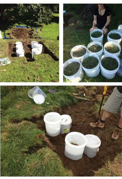
(7) 3.7.1. Extraction from soil ............................................................................................. 22. 3.7.2. Soil sample concentration and derivatisation .................................................... 26. 3.7.3. Extraction from leachate..................................................................................... 26. 3.7.4. Leachate sample concentration and derivatisation............................................ 27. 3.7.5. Analysis of Triclosan residues by Gas Chromatography Mass-Spectrometry. .... 29. 3.8.. Molecular analysis of Escherichia coli ......................................................................... 30. 3.8.1. Microbial DNA extraction from leachate ...................................................................... 30. 4.. 3.8.2. Microbial DNA extraction from soil ........................................................................ 31. 3.8.3.. Quantitative Polymerase Chain Reaction (qPCR).................................................... 31. Determining the EC50 of triclosan (TCS) in a silty clay loam ................................................ 33 4.1. Introduction ................................................................................................................ 33. 4.2. Materials and methods ............................................................................................... 35. 4.2.1. Soil sampling and initial characterisation ........................................................... 35. 4.2.2. Triclosan addition to soil ..................................................................................... 35. 4.2.3. Analysis ............................................................................................................... 36. 4.2.4. Statistics .............................................................................................................. 37. 4.3. 5.. Results ........................................................................................................................ 38. 4.3.1. Soil sampling and initial characterisation ........................................................... 38. 4.3.2. Substrate Induced Respiration ............................................................................ 38. 4.3.3. Microbial biomass ............................................................................................... 38. 4.3.4. Microbial metabolic quotient (qCO2) .................................................................. 39. 4.3.5. Sulphatase enzyme activity ................................................................................. 40. 4.3.6. EC50 determinations ............................................................................................ 40. 4.4. Discussion................................................................................................................... 42. 4.5. Conclusion ................................................................................................................... 44. Lysimeter study ................................................................................................................... 45 5.1. Introduction ................................................................................................................ 45. 5.2. Materials and methods ............................................................................................... 47. 5.2.1. Source of soils ..................................................................................................... 47. 5.2.2 Lysimeter facility ........................................................................................................ 48 5.2.3 Irrigation volumes and for lysimeters. ....................................................................... 49 5.2.4 Composition of greywater treatments. ..................................................................... 50 5.2.5 Experimental procedure ............................................................................................ 51 5.2.6 Escherichia coli preparation and enumeration. ......................................................... 52 v.

(8) 5.2.7 Escherichia coli survival .............................................................................................. 53 5.3. Analytical methods ..................................................................................................... 54. 5.3.1 Substrate induced respiration, sulphatase, biomass, triclosan analysis and Escherichia coli quantification ............................................................................................ 54 5.3.2 Statistics ..................................................................................................................... 54 5.4. Results ......................................................................................................................... 54. 5.4.1 Escherichia coli survival in soil and greywater ........................................................... 54 5.4.2. Lysimeters ........................................................................................................... 55. 5.4.3. Soil health indicators........................................................................................... 65. 5.5. Discussion.................................................................................................................... 72. 5.5.1 Escherichia coli in soil ................................................................................................. 72 5.5.2 Escherichia coli in leachate ........................................................................................ 74 5.5.3 Triclosan in soil ........................................................................................................... 76 5.5.4 Triclosan in leachate .................................................................................................. 77 5.5.5 Soil health indicators.................................................................................................. 79 5.6 6.. Conclusion ................................................................................................................... 80. Education intervention ....................................................................................................... 83 6.1. Introduction ................................................................................................................ 83. 6.1.1 The school. ................................................................................................................. 84 6.1.2 Student engagement.................................................................................................. 84 6.1.3. Greywater experiment Introduction................................................................... 85. 6.2.. Aim .............................................................................................................................. 86. 6.3.. Materials and method ................................................................................................ 86. 6.3.1. Student engagement................................................................................................. 86 6.3.2 Greywater experimental design................................................................................. 87 6.3.3. Hui ............................................................................................................................. 90 6.3.4. Student worksheet and survey ................................................................................. 92 6.4.. Results ......................................................................................................................... 93. 6.4.1. Student involvement................................................................................................. 93 6.4.2. Experimental results ................................................................................................. 93 6.5.. Discussion.................................................................................................................... 94. 6.5.1 Student engagement.................................................................................................. 94 6.5.2 Greywater experiment ............................................................................................... 95 6.5.3 Hui .............................................................................................................................. 95. vi.

(9) 6.5.4 Student worksheet and survey .................................................................................. 96 6.6. Summarising conclusion ............................................................................................. 96. 6.7. Acknowledgements..................................................................................................... 98. 7.. General discussion .............................................................................................................. 99. 8.. Conclusions ....................................................................................................................... 102. 9.. References ........................................................................................................................ 103. 10.. Appendix ........................................................................................................................... A. 10.1 Presentation school children gave at the hui ................................................................... A 10.2 Worksheet and survey filled out by school children with guidance from Donna Andrews .................................................................................................................................... H Worksheet:............................................................................................................................. I Survey:................................................................................................................................... O. vii.

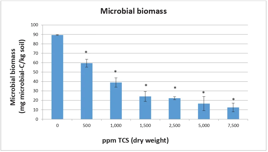
(10) List of Figures Figure 1: New Zealand rainfall 1971 – 2000 (Source: NIWA)........................................................ 7 Figure 2: Chemical structure of triclosan (source: www.niehs.nih.gov) ..................................... 13 Figure 3: Biodegradation and biotransformation of TCS in soil. ................................................. 15 Figure 4: The conversion of the colourless substrate, potassium p-nitrophenyl sulphate, to the yellow p-nitrophenol compound by the sulphatase enzyme. .................................................... 20 Figure 5: The derivatisation process of TCS with MTBSTFA before analysis .............................. 29 Figure 6: Substrate induced respiration (SIR) at investigated TCS levels. The brackets on the graph indicate subsets of data where a statistically significant (p<0.05) change in respiration in relation to time was observed. ................................................................................................... 38 Figure 7: Microbial biomass at investigated TCS levels on day 17. Asterisk indicates difference of statistical significance (p<0.05) from the control calculated using Tukey’s HSD test. ........... 39 Figure 8: Microbial metabolic quotient at investigated TCS levels on day 17. The asterisk indicates differences of statistical significance (p<0.05) from the control calculated using Tukey’s HSD test. ........................................................................................................................ 40 Figure 9: Sulphatase activity at investigated TCS concentrations on day 17. The asterisk indicates statistical significance from the control calculated using Tukey’s HSD test................ 40 Figure 10: EC50 determined with sulphatase activity at investigated TCS levels. ....................... 41 Figure 11: EC50 determined with microbial biomass at investigated TCS levels. ........................ 41 Figure 12: Sample sites, clock-wise from top left; Gisborne, Lincoln, Katikati ........................... 47 Figure 13: The excavation process of the lysimeters used in this study..................................... 49 Figure 14: Left: Lysimeters positioned in the facility. Right: the compartment at the bottom of the funnel in which the lysimeters sits is large enough to just accommodate sample collection containers. .................................................................................................................................. 49 Figure 15: Copies of the uidA gene in E. coli detected in each layer of the Gisborne soil indicated for all 4 treatments. Error bars were calculated using standard deviation. The graph’s y-axis begins at the average detection limit for all datasets analysed. ...................................... 56 Figure 16: Copies of the uidA gene in E. coli detected in each layer of the Katikati soil indicated for all 4 treatments. Error bars were calculated using standard deviation. The graph’s y-axis begins at the average detection limit for all datasets analysed. ................................................ 56 Figure 17: Copies of the uidA gene in E. coli detected in each layer of the Lincoln soil indicated for all 4 treatments. Error bars were calculated using standard deviation. The graph’s y-axis begins at the average detection limit for all datasets analysed. ................................................ 57 Figure 18: Copies of the uidA gene in E. coli detected in fortnightly leachate composites of the Gisborne soil. .............................................................................................................................. 58 Figure 19: Copies of the uidA gene in E. coli detected in fortnightly leachate composites of the Katikati soil. ................................................................................................................................. 59 Figure 20: Copies of the uidA gene in E. coli detected in fortnightly leachate composites of the Lincoln soil................................................................................................................................... 59 Figure 21: Concentration triclosan detected in each horizon of the Gisborne soil indicated for all 4 treatments. Error bars were calculated using standard deviation. .................................... 60 Figure 22: Concentration triclosan detected in each horizon of the Katikati soil indicated for all 4 treatments. Error bars were calculated using standard deviation. ......................................... 61. viii.

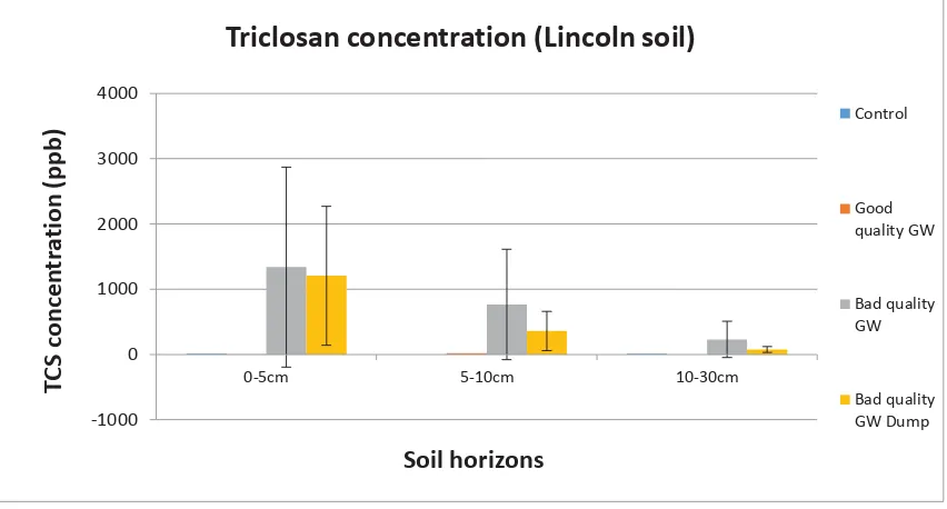
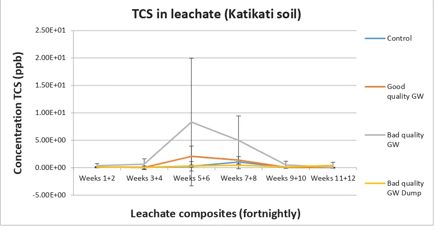
(11) Figure 23: Concentration triclosan detected in each horizon of the Lincoln soil indicated for all 4 treatments. Error bars were calculated using standard deviation. ......................................... 61 Figure 24: Concentration TCS detected in fortnightly leachate composites of the Gisborne soil. .................................................................................................................................................... 62 Figure 25: Concentration TCS detected in fortnightly leachate composites of the Katikati soil. 63 Figure 26: Concentration TCS detected in fortnightly leachate composites of the Lincoln soil. 64 Figure 27: Concentration Met-TCS detected in fortnightly leachate composites of the Lincoln soil. .............................................................................................................................................. 64 Figure 28: Fortnightly rainfall for Mana Island. Mana Island was the closest weather station to where the experiment was conducted (Data supplied by Metservice). ..................................... 65 Figure 29: Substrate induced respiration for the 0-5cm horizon of the Gisborne soil cores. Error bars were constructed using standard deviation. ...................................................................... 66 Figure 30: Substrate induced respiration for the 0-5cm horizon of the Katikati soil cores. Error bars were constructed using standard deviation. ...................................................................... 66 Figure 31: Substrate induced respiration for the 0-5cm horizon of the Lincoln soil cores. Error bars were constructed using standard deviation. ...................................................................... 67 Figure 32: Microbial biomass for the 0-5cm horizon of the Gisborne soil cores. Error bars were constructed using standard deviation. ....................................................................................... 67 Figure 33: Microbial biomass for the 0-5cm horizon of the Katikati soil cores. Error bars were constructed using standard deviation. ....................................................................................... 68 Figure 34: Microbial biomass for the 0-5cm horizon of the Lincoln soil cores. Error bars were constructed using standard deviation. ....................................................................................... 68 Figure 35: Sulphatase activity for the 0-5cm horizon of the Gisborne soil cores. Error bars were constructed using standard deviation. ....................................................................................... 69 Figure 36: Sulphatase activity for the 0-5cm horizon of the Katikati soil cores. Error bars were constructed using standard deviation. ....................................................................................... 69 Figure 37: Sulphatase activity for the 0-5cm Horizon of the Lincoln soil cores. Error bars were constructed using standard deviation. ....................................................................................... 70 Figure 38: Microbial metabolic quotient for the 0-5cm horizon of the Gisborne soil cores. Error bars were constructed using standard deviation. ...................................................................... 70 Figure 39: Microbial metabolic quotient for the 0-5cm horizon of the Katikati soil cores. Error bars were constructed using standard deviation. ...................................................................... 71 Figure 40: Microbial metabolic quotient for the 0-5cm horizon of the Lincoln soil cores. Error bars were constructed using standard deviation. ...................................................................... 71 Figure 41: Flow patterns created after 3 additions of greywater at the recommended rate for that soil type, and marking the infiltration front as soon as the irrigation stopped, and 5mins after. This was done for all 3 soils. .............................................................................................. 74 Figure 42: The 9 kōhūhū plants chosen for the experiment. Plants were grouped in 3 treatments with 3 replicates for each treatment. ...................................................................... 88 Figure 43: The plants were irrigated twice each weekday for 7 weeks...................................... 89 Figure 44: Measurements of stem height, assessment of appearance and leaf count were recorded twice weekly ................................................................................................................ 90 Figure 45: The result boards containing the observational data and conclusions made by the students. These were presented at the hui to the community along with a PowerPoint presentation................................................................................................................................ 91 ix.

(12) Figure 46: One of the students asked to represent her class and give the presentation containing the results and conclusions at the hui. ..................................................................... 92. x.

(13) List of Tables Table 1: Greywater quality (Sources: Western Australia department of health (2005). Code of Practise for Reuse of Greywater in Western Australia, and Australian National Guidelines for Water Recycling (2006)) ................................................................................................................ 6 Table 2: Sequences of the primers used in the method optimisation for qPCR analysis ........... 32 Table 3: The EC50 values for sulphatase and biomass as determined by the 50% decline in activity of the soil microbial community. The EC20 is a concentration of TCS (ppm) where 20% of the community’s activity is affected. The R2 refers to figures 10 and 11. ............................. 41 Table 4: Physical properties of the 3 soils chosen for the experiment ....................................... 50 Table 5: Composition of greywater used for lysimeter study (See footnotes1 & 2 for references) .................................................................................................................................. 51 Table 6: The survival of E. coli in soil after addition of greywater containing 10ppm triclosan . 55 Table 7: Constituents of synthetic greywater. *Selection of specific brands does not represent an endorsement by this research project. .................................................................................. 89. xi.

(14) 1.. 1.1. Introduction and Aims. Introduction. Managing municipal water resources and minimising the impacts of wastewater discharge are critical elements of sustainable modern communities. The separation of greywater streams, specifically those from bathroom sinks, showers and laundry, from blackwater streams originating from toilets and kitchen sinks, is emerging as a potential water management tool (Casanova, Gerba, & Karpiscak, 2001; Chaillou, Gérente, Andrès, & Wolbert, 2011; Donner et al., 2010; Eriksson, Auffarth, Henze, & Ledin, 2002). There is an increase in the usage of greywater for irrigation especially in countries with arid regions, such as China, Australia and the south-western United States (Harrow & Baker, 2010; Waller & Kookana, 2009). In New Zealand, where water shortages are not typically an issue, greywater diversion is practiced as a means of excess water disposal, with little or no knowledge regarding environmental impact (Cass, Beecroft, & Lowe, 2012). Current regional guidelines generally propose the use of diverted greywater for sub-surface irrigation of land, and restrict the use of greywater for irrigation to the property from which it originated (e.g. Kapiti Coast District Council). The reasoning behind such restrictions is that greywater contains an extremely variable and complex mixture of microbes and chemicals, potentially at high concentrations (Casanova et al., 2001; Gross, Kaplan, & Baker, 2007). These compounds can be considered to be a contaminant if present in the environment at high concentrations. Therefore, while greywater diversion is potentially beneficial from a water conservation and sustainability point of view, its use may be a high-risk activity with potential detrimental impacts on the environment and public health. While greywater management is extensively practiced around the world, there is little NZ experience or scientific information, in particular regarding the impacts of biological and chemical contaminants of greywater on soils, groundwater and public health. There are no national guidelines or model health risk assessments for greywater use; hence the design of greywater application systems is difficult and inconsistent across the country.. 1.

(15) Greywater contains a range of contaminants, including metals such as Zinc and Copper, nutrients such as phosphates and nitrates, and, micro-organisms such as Escherichia coli (Eriksson et al. (2002). Untreated greywater also contains other organic contaminants including pharmaceuticals, fragrance fixing agents, preservatives and antimicrobial chemicals (Donner et al., 2010; Eriksson, Auffarth, Eilersen, Henze, & Ledin, 2003). These compounds are of concern as the practice of greywater reuse could possible introduce them into the environment. One such a compound is triclosan (TCS; 5-chloro-2-[2, 4-dichlorophenoxy]-phenol) (Harrow, Felker, & Baker, 2011).According to Harrow and Baker (2010), TCS is the most commonly used antibacterial compound in the United States. In New Zealand, such antibacterial compounds are found in many common personal care products including toothpastes, hand washes and in sports clothing (McMurry, Oethinger, & Levy, 1998). Once these compounds enter a domestic greywater stream where the water is reused, there is a direct route for TCS to the receiving environment. Not a lot is known about how triclosan affects microbial communities in soil when greywater containing the compound is used for irrigation (Harrow & Baker, 2010), and due to the compounds high affinity for organic matter (Butler, Whelan, Ritz, Sakrabani, & van Egmond, 2011) the unsafe irrigation of greywater could result in the accumulation of TCS in receiving soils. Studies have shown that microbial function such as respiration, community composition and enzyme activity in soil is affected by the presence of TCS (Ali, Arshad, Zahir, & Jamil, 2011; McMurry et al., 1998; Waller & Kookana, 2009). Federle, Kaiser, and Nuck (2002) also found that TCS affects basic microbial functions analysing the effect of TCS on nitrifying bacteria by measuring bacterial respiration rates. Gaining a greater understanding of the impacts of greywater diversion and disposal practices on the environment, particularly focusing on the long-term implications for soil, groundwater and public health, is essential for sustainable management of greywater reuse in New Zealand.. 2.

(16) 1.2. Aims. 1.2.1. Determination of the EC501 for triclosan in soil to inform the dosing rate for the. lysimeter experiment. 1.2.2. Firstly, investigating the partitioning of TCS and E. coli through the soil profile of 3. different soils, and what the potential was for TCS and E. coli to leach through the soil profile, and secondly, investigating the effect potentially accumulated TCS has on soil health parameters. 1.2.3. Raising awareness to support behavioural change in a community (regarding the fate. and effects of household chemicals in the environment) through the engagement with primary-level students while providing them with an authentic scientific experience.. 1.3. Research approach. Greywater can be a valuable resource regardless of the drivers that motivate its reuse. Its reuse by application to soil however needs to be done with care, taking into account the public health risks and possible long term effects on soils. These effects have not yet been characterised in New Zealand soils. The research in this thesis was carried out to investigate the effect of TCS found in greywater on the receiving soil environment. The knowledge gained from this study will aide in the construction of consistent general greywater irrigation guidelines. A combination of soil microbiology, biochemistry, molecular biology and analytical chemistry techniques were employed in this study with the aim of gaining more information on the fate and effects of greywater contaminants. A representative organic contaminant (TCS) and an indicator microbial contaminant (E. coli) were investigated. The first phase of the study explored how the soil microbial community reacted to TCS exposure over time and the effects that TCS had on soil health parameters such as; soil bacterial respiration, enzyme activity and a stress biomarker; metabolic quotient. These indicators of soil health are used routinely in soil ecology for monitoring the impacts of land treatment, such as the application of sewage biosolids to soils (Speir, van Schaik, Hunter, Ryburn, & Percival, 2007).. 1. The EC50 of a contaminant is the concentration at which at least 50% of a specific microbial function is affected. It is the point half way between the baseline and the maximum of a microbial response after exposure to the toxin. It is a measure of toxic potency.. 3.

(17) In the second phase of the study, the fate and effect of TCS and E. coli irrigated onto soil cores (lysimeters) with greywater were investigated. This aimed to understand the partitioning of TCS through the soil profile of 3 different soils, and what the potential was for TCS and E. coli to leach through the soil profile. The potential public health risk of pathogen exposure was explored by including various concentration of E. coli in the treatments. There have been numerous studies of the fate of microorganisms in the waste water treatment process; however there is a knowledge gap on the survival of pathogens like E. coli in soil after irrigation with greywater. It is neither practical nor economical to continually monitor greywater for the presence of pathogens. It would therefore be valuable to gain an indication on the fate of a model organism such as E. coli in the soil environment after introduction to the soil environment by the irrigation of greywater. Escherichia coli is a practical indicator organism as it has a high abundance in comparison to other pathogens that might be introduced to soil. It is expected to behave in the same way as other pathogens due to similarities in life processes and it is easy and cost-effective to detect. In chapter 3, the major methods employed in this study are presented. Chapter 4 investigates the effect of TCS on a silty clay loam soil. This chapter included an analysis of the SIR, sulphatase, microbial metabolic quotient and how the SIR for this soil changed over a period of 20days after initial exposure to various concentrations of TCS in a dose-response experiment. The lysimeter study where the fate and effect of TCS was investigated in the soil environment is described in Chapter 5. The chapter includes the experimental protocols employed, results and a discussion on the observations made. The analysis performed in this study included the movements of TCS through the soil profile by measuring TCS in 3 different soil horizons, and the leaching of TCS by analysis of the TCS content of weekly collected leachate samples. Soil health parameters such as microbial biomass, sulphatase activity and SIR2 were measured for the top 5cm of the soil cores. The movement of E. coli through the soil profile was also monitored by quantification of E. coli by qPCR3. This analysis was performed for the 3 soil horizons as well as the leachate. Chapter 6 discusses the involvement of the scientific community at primary level education in order to raise awareness of the effects that greywater constituents might have on the receiving environment. The engagement involved helping the student formulate a scientific hypothesis, how to design an experiment and draw conclusions from observations. The 2 3. Substrate induced respiration. Quantitative polymerase chain reaction. 4.

(18) students learned about what contaminants might be in greywater while relating the knowledge gain back to the curriculum. The aim of the engagement was to promote consciousness of what is put down the drain. The final discussion and future recommendations are presented in chapter 7, and Chapter 8 contains the final conclusions.. 5.

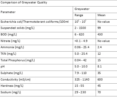
(19) 2. 2.1. Literature review. What is greywater?. Greywater is defined as the water originating from wash basins, showers and laundry effluent in a household (Chaillou et al., 2011) and includes all untreated household waste water except for toilet water (McCormack, 2011). It typically contains high concentrations of soaps, oils and detergents from personal care products such as body-washes, laundry detergent, and hair care products (Gross et al., 2005). The composition of greywater varies within a household, depending on where it originates from. Greywater from laundry will contain lint, laundry detergents, sodium, and other nutrients such as nitrates and phosphates. Greywater from baths and showers will contain hair, toothpaste, body fat, oils, and faecal coliforms such as Escherichia coli. See Table 1 for chemical and nutrient composition. The composition and volume of greywater varies greatly between households (Casanova et al., 2001; Eriksson, Andersen, Madsen, & Ledin, 2009; Jefferson, Palmer, Jeffrey, Stuetz, & Judd, 2004). This is not surprising as the composition mainly depends on the number of inhabitants, their habits and age. Table 1: Greywater quality (Sources: Western Australia department of health (2005). Code of Practise for Reuse of Greywater in Western Australia, and Australian National Guidelines for Water Recycling (2006)). Comparison of Greywater Quality Greywater. Parameter. Range. Mean. Escherichia coli/Thermotolerant coliforms/100ml. 101 - 107. No value. Suspended solids (mg/L). 2 - 1500. 99. BOD (mg/L). 6 - 620. 430. Nitrate (mg/L). <0.1 - 4.9. No value. Ammonia (mg/L). 0.06 - 25.4. 2.4. TKN (mg/L). 5.0 - 25.4. 12. Total Phosphorus (mg/L). 0.04 - 42. 15. pH. 5.0 - 10.0. 8.1. Sulphate (mg/L). 7.9 - 110. 35. Conductivity (mS/cm). 325 - 1140. 600. Hardness (mg/L). 15 - 55. 45. Sodium (mg/L). 29 - 230. 70. 6.

(20) The average greywater production in industrialised countries average between 100-150L of greywater per person per day (Friedler, 2004).. 2.2. Greywater reuse drivers. New Zealand is a country of dramatically different climatic regions with climates varying in the North from warm sub-tropical, to a cool temperate climate in the South. There is also significant differences in annual rainfall in New Zealand with the west coast of the South Island receiving more than 6000mm of rain per year (Mackintosh, 2001).In contrast to this, areas less than 100km from the west coast experience rainfalls as low as 400mm annually (Mackintosh, 2001).There is a clear spatial difference in rainfall (Fig. 1).. Figure 1: New Zealand rainfall 1971 – 2000 (Source: NIWA). In the North and central areas of the country, the rainfall is predominantly spread out throughout the year with a dry period during the summer. In the South Island, winter gets. 7.

(21) least rainfall (Mackintosh, 2001). This indicates that there are spatial as well as temporal differences in national rainfall patterns. With soil in New Zealand being such an important resource, it is important to remember that the country’s soil can be as variable is its climate. Soils are classified using various properties of the soils (McLaren & Cameron, 1996). These properties might include the chemical and physical properties such as soil texture, structure and history. Water holding capacity (WHC) is related to the soil texture and composition as it is dependent on the size of the pores in the soil (McLaren & Cameron, 1996). WHC determines how much water the soil is able to retain. Soil function is related to the properties and moisture content of soil and is thus influenced by the amount of water it receives.. 2.2.1. Water shortages. Where soils with low WHC occur in a low rainfall region, there might routinely be soil water deficits (SWD) causing water shortages. These water shortages could become more pronounced by a changing climate, urbanisation and the cultivation of an increased awareness to conserve water (Harrow et al., 2011). With modernisation, household water budgets in both industrialising and industrialised nations are on the increase, and fresh water resources for domestic use are becoming all the scarcer. Along with other options such as the use of rainwater from collection tanks, the reuse of greywater as a resource reduces the requirements for potable water in a household. There is an increase in the usage of greywater for irrigation especially in countries with arid regions, such as China, Australia and the southwestern United States (Harrow et al., 2011; Waller & Kookana, 2009).. 2.2.2. Surplus water. In New Zealand, where water shortages are not typically an issue, greywater diversion is often practiced as a means of excess water disposal (Siggins et al., 2013). The practice can assist in alleviating the strain on the receiving environment after waste water treatment, as well as on waste water treatment infrastructure. The practice could be beneficial for reticulated as well as unarticulated areas. Siggins et al. (2013) found that the treatment efficacy and life of old and poor-functioning septic tanks could be improved by diverting the greywater fraction of the household waste water. The greywater diversion in this study was done with a manufactured. 8.

(22) Watersmart® greywater diversion system. The system makes use of sub-surface irrigation of the greywater onto soil. An increased awareness of the need to conserve potable water also drives greywater reuse. This is, however, frequently done without proper knowledge of greywater constituents, its environmental fate and effects and the potential public health risks associated with irrigating greywater without proper knowledge of how to do so responsibly (Cass et al., 2012).. 2.3. Risks and benefits associated with greywater reuse. 2.3.1. Risks. There are potential health and environmental risks associated with the reuse of greywater. These risks arise when a reuse system functions poorly, or is overloaded. The risk is mainly attributable to the over irrigation of soil to beyond its capacity. This results in waterlogging of the soil and ponding of greywater on the surface (Cass et al., 2012). The greywater could then potentially damage soil systems, bring people into contact with pathogens such as E. coli, and the untreated greywater might make its way to receiving water ways. In a public survey conducted in (Cass et al., 2012), 42 households were interviewed on their opinions regarding water conservation, environmental health risks, regulations, and greywater promotions and information associated with greywater reuse. The perceived risks associated with greywater reuse as identified in the survey include the following: • Health concerns, particularly from households with a higher risk of faecal content in their greywater; • Odour (including due to hydrogen sulphide); • Pets bring potential contaminants into the house after being in contact with the greywater applied outside; • Contamination of neighbouring properties and potential complaints; • Soil contamination; • What will happen when someone takes over a greywater system in their new home and are not interested in its management; • Long term impacts on the soil; • The difficulty of managing the soaps and fat content of the greywater;. 9.

(23) • The Regional Council will make changes that will negate greywater systems that have been installed; • NZ greywater systems require more precision than Australian systems; • Less water in the reticulated system will cause blockages; • The nutrients from the greywater area are an important part of the solid waste breakdown therefore inappropriate to remove it; • Sodium will damage soils to which greywater is applied; and • Phosphorus (Results taken directly from report by Cass et al. (2012)). 2.3.2. Benefits. It is clear that there are positive and negative aspects to the reuse of greywater. Some of the positives include that the reuse of greywater will reduce the demand for the use of potable water (McCormack, 2011). There could also be significant benefits for municipal waste plants. The volume of discharge water would be greatly reduced if greywater diversion/reuse were to be employed on a large enough scale. The nutrients occurring in greywater will not reach coastal waters like 60% of New Zealand sewage (McCormack, 2011). The reuse and subsequent irrigation of greywater also hold benefits for the garden. It will relieve water stress in plants if the soil is at a soil-water deficit, and nutrients from the greywater will have positive effects on plant nutrition. It thus has positive economic implications if the practise is employed in an area where water is metered for example Kapiti Coast. The load on old and failing septic tanks may also be alleviated, allowing the septic tank to operate more efficiently (Siggins et al., 2013).. 2.4. Greywater composition. 2.4.1. Microbiological quality. The presence of faecal coliforms is routinely used as a general indicator of the microbial quality of water (Glassmeyer et al., 2005). The detection of faecal coliforms (FCs) in water indicates a potential health risk to humans. In greywater, the abundance of FCs are relatively low, however, the levels might rise to those typically found in blackwater as a result of washing nappies and clothing that might have been contaminated with faeces or vomit (Birks, Colbourne, & Hobson, 2004; Birks & Hills, 2007). 10.

(24) In the majority of New Zealand households where greywater diversion or reuse is practised, greywater is irrigated onto soil without being treated. Several studies have shown that untreated greywater may contain faecal contamination by the presence of indicator organisms such as E. coli (Birks & Hills, 2007; Casanova et al., 2001; Eriksson et al., 2009). A study conducted by Birks and Hills (2007) characterised the greywater from a block of flats with a dual-reticulation system. That study confirmed that levels of E. coli as high as 107 CFU/100ml could be found in a “real” source of greywater. There is thus a potential to increase the number of faecal coliforms in soil by irrigation of untreated greywater (Negahban-Azar, Sharvelle, Stromberger, Olson, & Roesner, 2012). It has been shown that microbes can survive in soil for long periods of time. E. coli has been reported to survive for weeks and under the ideal conditions (Mawdsley, Bardgett, Merry, Pain, & Theodorou, 1995). X. Jiang, Morgan, and Doyle (2002) found that E. coli was able to survive in soil amended with manure for longer than 200 days. The survival of Salmonella typhimurium have been illustrated to reach beyond 70 days in an experiment conducted by Turpin, Maycroft, Rowlands, and Wellington (1993) where the bacteria was cultured in constructed microcosms at 22°C and at 15% moisture content. Negahban-Azar et al. (2012) measured the number of faecal indicator organisms in soil that has been irrigated with greywater for 30yrs and compared it to soil on the same section that had been irrigated with fresh water. The study investigated soil from a selection of states, and in one soil from Texas, E. coli levels of 543 CFU/g soil were detected in the top 15cm of the soil horizon. More interesting is the detection of E. coli levels up to 1093 CFU/g soil in the 30100cm layer. E. coli levels found in the areas where freshwater was irrigated ranged from between 136 CFU/g soil and 160 CFU/g soil for the 0-15cm and 30-1400cm layers respectively. When numbers of E. coli are elevated in soil, there is an increased risk for E. coli to leach through the soil profile and be carried off site. A study conducted by Jiang et al. (2010) have shown that some soils are prone to preferential flow and that indicates that there is potential for E. coli to leach through the soil profile and potentially impairing groundwater quality. Pang et al. (2008) conducted a study where the transport of microbes was modelled through the soil profile of ten undisturbed soils. Microbial breakthrough curves were assessed for the lysimeters and it was concluded that rapid breakthrough of microbes in the leachate in structured soils with low moisture content could be as a result of bypass flow. The conclusions of that study support the hypothesis that transport of microbes through the soil profile by preferential flow is mediated by a compromised integrity of the soil’s macroporosity.. 11.

(25) Birks and Hills (2007) argued that the presence of E. coli in greywater does not infer the presence of pathogens, however if pathogens are present in greywater, their movement through the soil could be compared to the movement of E. coli. Monitoring the movement of E. coli thus provides an easy and relatively economical way of assessing the health risk associated with the irrigation of untreated greywater into soil.. 2.4.2 Nutrients in greywater Amongst other nutrients, greywater contains phosphorus and nitrogen-containing compounds such as nitrates and ammonia arising from the use of detergents such as washing powder, shampoo, and other personal care products (Rodda, Salukazana, Jackson, & Smith, 2011). These nutrients might be beneficial for plants and could potentially reduce the use of commercial fertilisers.. 2.4.3 Chemicals in greywater According to Eriksson et al. (2002), greywater contains a range of contaminants, including metals such as Zinc and Copper. It also contains other organic contaminants. These include pharmaceuticals, fragrance fixing agents, preservatives and antimicrobial chemicals (Donner et al., 2010; Eriksson et al., 2003). These compounds are of concern as the practice of untreated greywater reuse could directly introduce them into the environment. One such a compound of concern is triclosan (TCS; 5-chloro-2-[2, 4-dichlorophenoxy]-phenol) (Harrow et al., 2011).According to Harrow and Baker (2010), TCS is the most commonly used antibacterial compound in the United States. In New Zealand, such antibacterial compounds are found in many common personal care products including toothpastes, hand washes and in sports clothing (McMurry et al., 1998). Once these compounds enter a domestic greywater stream where the water is reused, there is a direct route for TCS to the receiving environment. With the use of 2 supermarket products (e.g. toothpaste and mouth wash) containing TCS, used at realistic amounts, it is possible that approximately 450mg of TCS could enter the environment from a single household’s greywater over a period of 10 years.. 12.

(26) 2.5 Triclosan (TCS), Chemical properties Triclosan is a white crystalline powder with a bulk density of 1.55 x 103 kg/m3 and a solubility of 0.0010g/L in water at 20°C (TOXNET, 2004). However, TCS has an increased solubility of more than 100g/L in organic solvents such as acetone. Triclosan is also known as Irgasan. Triclosan is a polycyclic organic compound (fig.2) that was introduced and used for its antibacterial and antifungal properties in the 1960s (Ledder, Gilbert, Willis, & McBain, 2006). Its effectiveness against bacteria such as E. coli is presumably due to fatty acid synthesis, and cell lysis at higher concentrations (McMurry et al., 1998).Triclosan may also influence the transcription of genes related to lipid, carbohydrate and amino acid metabolism (Reiss, Lewis, & Griffin, 2009).. Figure 2: Chemical structure of triclosan (source: www.niehs.nih.gov). Recent studies have also suggested that there is a link between TCS resistance in microbial communities and antibiotic resistance in bacteria (McMurry et al., 1998). In contrast, Ledder et al. (2006) concluded that bacterial colonies exposed to TCS did not undergo a significant increase in resistance to a range of antibiotics, including tetracycline, ciprofloxacin, nalidixic acid and chloramphenicol. Not a lot is known about how triclosan affects microbial communities in soil when greywater containing the compound is used for irrigation (Harrow & Baker, 2010). Triclosan has a dissociation constant (pKa-value) of 8.14 according to Butler et al. (2011). It is therefore a weak acid, more stable in the protonated form. The effects of soil pH could therefore affect the mobility of TCS due to its ionisable nature. The deprotonation of TCS at high pH to produce the phenolate-ion, a negatively charged particle, will facilitate the compound’s transport through the soil profile due to repelling effects of some organic colloids 13.

(27) and clay particles. This indicates that TCS might not strongly associate with soil particles. In contrast, Agyin-Birikorang, Miller, and O'Connor (2010) concluded that TCS desorption is much slower than the desorption in a retention-release study. This indicates that triclosan does form strong associations with organic matter. In addition, Butler et al. (2011) noted that TCS would have a high affinity for organic matter due to its log KOW of 4.78 (log octanol:water partition coefficient). This could result in the accumulation of TCS in receiving soils. In that study it was found that the addition of TCS to soil does have an effect on the substrate induced respiration (SIR) of soil microbial communities. This indicates the bioavailability of TCS in the soil environment.. 2.5.1. Fate of TCS in soil. There are many factors affecting the fate of TCS in soil such as the soil composition, climatic factors, and other abiotic factors such as soil moisture. Triclosan could be transported through the soil profile to enter groundwater reserves, or it could be degraded or transformed by soil microbes to other compounds. Another form of degradation is by sunlight. The variety and composition of microbial communities in soil could impact on the amounts and types of biodegradation products formed. Abiotic factors also the fate of TCS in soil (Butler, Whelan, Sakrabani, & van Egmond, 2012). These include the soil temperature, moisture content and the type of land-use.. 2.5.1.1 Transport through soil Butler, Whelan, Sakrabani, et al. (2012) found that traces of TCS leaches through the soil profile over time despite its strong affinity for adsorption to soil particles. Soil texture and composition also affects the fate of TCS. In that study it was indicated that TCS leaches through the soil profile and that the soil texture could influence the fate of the compound’s partitioning. It was indicated that TCS more strongly associates with clay soils when compared to sandy soils and loamy sand soil. Yet Kwon and Xia (2012) found no leaching of TCS through the soil horizon. In that study soil columns containing sandy soil were amended with a layer of soil which had been spiked with TCS to a concentration of 760mg/kg TCS per dry weight of soil. The columns were subsequently irrigated with water. After 101 days of irrigation, the soil horisons and leachate from the cores were analysed for TCS. They concluded that their inability to detect TCS in the 14.

(28) leachate was due to high sorption to soil and that TCS had limited transport through the soil profile. The soil columns used for this study were not intact, but instead repacked and can therefore not be compared to studies using intact soil cores. Kwon and Xia (2012) did, however, find that there was leaching of TCS in soil columns amended with biosolids containing TCS, bolstering the theory the TCS adsorbs to organic particulates. Due to TCS’s affinity for organic compounds, particulate matter and the variability of soil characteristics of New Zealand soils, it follows that TCS bioavailability and transport within the soil profile would vary between soils.. 2.5.1.2 Degradation. Triclosan is available to bacteria for uptake and is readily degraded or transformed to products that might be even more persistent in the environment that TCS itself (Gangadharan Puthiya Veetil, Vijaya Nadaraja, Bhasi, Khan, & Bhaskaran, 2012). Typically the breakdown products in soil include 2, 4-dichlorphenol (2, 4-DCP) and 4-chlorocatechol (Fig 3).. Figure 3: Biodegradation and biotransformation of TCS in soil.. Triclosan is also photolytically degraded to 2, 4-DCP and 2, 8-dichlorodibenzo-p-dioxin (2,8DCDD) (Latch, Packer, Arnold, & McNeill, 2003).. 2, 4-DCP in a liquid form and 2,8-DCDD is. absorbed through the skin, and excessive exposure might have serious health complications and could even result in death (Latch et al., 2005).. 15.

(29) 2.5.2. Effects of TCS in soil. 2.5.2.1 Microbial respiration Microbial function in soil is affected by the presence of TCS. Ali et al. (2011) noted a statistically significant effect of TCS on soil microbial respiration by measuring a decrease 14Cglucose mineralisation with increased TCS concentration. Butler et al. (2011); McMurry et al. (1998) and Waller and Kookana (2009) concluded the same. The effect however, that Waller and Kookana (2009) observed was not as dramatic as the effects reported by Butler et al. (2011) where much higher concentrations were used. Using higher concentrations of TCS might be a better approach to describe the effects of TCS accumulation in soil and impacts on soil microbial communities.. It has also been. demonstrated by Federle et al. (2002) that TCS affects basic microbial functions analysing the effect of TCS on nitrifying bacteria by measuring bacterial respiration rates.. 2.5.2.2 Microbial community composition It is also possible that the composition of soil microbial communities is altered after exposure to TCS. Harrow et al. (2011) demonstrated that soil microbial communities and bacterial numbers changed in soils irrigated with greywater containing TCS. However McNamara and Krzmarzick (2013) found that the composition of a soil microbial community remains intact. That study was conducted using minute amounts of TCS and didn’t provide for the concentrations of TCS residues in soil after accumulation.. 2.5.2.3 Enzyme activity Soil enzyme activity could be used to assess the health of soil microbial communities (Winding, Hund-Rinke, & Rutgers, 2005). Liu, Ying, Yang, and Zhou (2009) demonstrated how the presence of TCS in soil affected the soil enzyme activity. In this study it was concluded that phosphatase activity was significantly inhibited by concentrations of TCS between 0.1mg/kg dry weight of soil and 50mg/kg dry weight of soil, although the soil microbial community recovered in the later stages of a 23 day incubation process. In contrast Waller and Kookana (2009) measured the effect of TCS on four enzymes. Only one enzyme, β-glucosidase responded negatively to the addition of TCS.. 16.

(30) 2.5.2.4 Microbial stress Soil microbial communities show signs of microbial stress when exposed to TCS. Park, Zhang, Ogunyoku, Young, and Scow (2013) observed an increase in microbial stress indicators when soil microbes were exposed to soils and biosolids amended with TCS. The increase in microbial stress biomarker used (cy17/precursor ratio) correlated positively with the increase in TCS concentration. This particular stress indicator was chosen as bacteria responding to stress from the environment react by transforming a cis-double bond in the cell membrane in order to achieve greater cell membrane stability. The indicator was measured by extraction cell membrane phospholipids and measuring by gas chromatography. The effect of TCS might be amplified in the presence of co-contaminants. A study conducted by Horswell et al. (2014) investigated possible effects that co-contaminants to TCS, such as copper (Cu) and zinc (Zn), might have on the soil microbial community. It this study, various amounts of Zn, and Cu were added to soil. Various amounts of TCS were also added to investigate the environmental effects of a complex cocktail of chemicals on a soil eco-system. It was concluded that the presence of toxic metals such as Zn and Cu enhance the persistence of TCS in the soil environment (Horswell et al., 2014). The chemical cocktail had a synergistic effect on soil health indicators.. 17.

(31) 3.. Methods. 3.1 Moisture content, dry matter content and water holding capacity The moisture, dry matter content and water holding capacity for each soil was determined from the bulk soil collected at each sample site.. 3.1.1. Moisture and dry matter content: Field moist soil was sieved to < 2mm in order to break up soil aggregates, remove vegetation and debris and homogenise the samples. For each soil type, triplicate subsamples containing a recorded weight of no less than 10g of soil, were weighed into porcelain crucibles. The samples were dried at 105°C for 24hrs to evaporate all moisture. Samples were allowed to cool to room temperature in a desiccator containing blue silica gel, and the dry weights were recorded to 3 decimal places. The dry matter and moisture content were calculated as below:. Fresh weight (g). =. (crucible + fresh soil) — crucible (g). Dry weight (g). =. (crucible + dry soil) — crucible (g). Soil Dry matter (DM %). =. Dry weight of soil (g) x 100 Fresh weight of soil (g). Soil Moisture content (MC%). =. 100 – DM. 18.

(32) 3.1.2 Water-holding capacity (WHC): WHC is the maximum potential volume of water held by 100g of soil. Eleven plastic funnels with a diameter between 7cm and 10cm were prepared by placing 0.25g (± 0.05g) cotton wool in the top of the stem. The cotton wool was then loosely compacted with a narrow spatula. The bottom ends of the funnels were plugged with Blu-tack® to prevent leakage and the funnels were then placed in 25ml measuring cylinders. Soil samples (25g ± 0.05g) were weighed in triplicate and placed in the funnels. The test also included two blank funnels that contained everything except soil. Exactly 25ml of water was poured into each funnel. The Blu-tack® plugs were removed 30min later to allow the filtrate to drip through into the measuring cylinders. The volume of water retained by 100g of soil was calculated as follows:. WHC = 4x (volume collected from blanks – volume collected from samples) + MC. 3.2. pH. Four grams (±0.05g) of moist soil was weighed into 50mL glass beakers and 10ml deionised water was added. The mixture was stirred with a glass rod, capped and left overnight to equilibrate. The pH was measured on a Thermo-Orion Model 310 pH meter by glass electrode.. 3.3.. Substrate induced respiration. Substrate induced respiration (SIR) was performed according to Degens and Harris (1997), and Campbell, Chapman, Cameron, Davidson, and Potts (2003). The apparatus used for soil loading and the trays containing the reaction wells in this analysis was produced by Macaulay Enterprises Limited and the method suggested by the manufacturer followed. The method entailed the capture of bacterial carbon dioxide (CO2) produced after the addition of an appropriate substrate (glucose in this case) and measurement of the absorbance of a microtitre plate filled with pH sensitive agar. The CO2 was absorbed into the agar and altered the pH in each well and a colour change from pink to yellow was observed. The difference between the initial absorbance of the well and the absorbance after 6h indicated the amount of CO2 produced during the test time period. 19.

(33) 3.4. Sulphatase enzyme activity. The sulphatase enzyme is an important indicator of soil biological processes, soil fertility and therefore soil health. Soil sulphatase activity was measured using the p-nitrophenyl colorimetric method employed by Speir (1984) and Tabatabai (1970) with slight modifications. Briefly, the method involves the addition of potassium p-nitrophenol sulphate as a substrate to the soil sample. Enzyme substrate (0.5ml) was added to 0.5g of each soil sample and the reaction was allowed to continue for 4hrs. During that time the substrate was converted to p-nitrophenol, by the activity of the sulphatase enzyme. P-nitrophenol is a yellow coloured complex in the presence of a base (NaOH) and is quantifiable by spectrophotometry (Fig 4). The quantity of p-nitrophenol can then be directly related to sulphatase enzyme activity. Calcium chloride (CaCl2) was added before the base to prevent the dispersion of clay particles in the soil as the organic material extracted by NaOH might have interfered with the colorimetric analysis of the yellow compound. Dispersed clay particles also hindered the filtration of the extract. Prior to spectrophotometric analysis, samples from the Lincoln soil samples were diluted 1:50 with Milli-Q water and the absorbance analysed at 400nm on a Varian Cary 50 spectrophotometer. Sulphatase activity of the 0-5cm fraction of soils from the lysimeter study (Chapter 4) was diluted 1:4 with deionised water and the absorbance analysed on a FLUOstar OPTIMA spectrophotometer by BMG LABTECH at 405nm.. Figure 4: The conversion of the colourless substrate, potassium p-nitrophenyl sulphate, to the yellow p-nitrophenol compound by the sulphatase enzyme.. 20.

(34) 3.5. Microbial biomass. Two replicates of soil were sieved to <2mm and adjusted to 60% WHC. Triplicate sub-samples of each sieved soil (2g ± 0.002g) were placed into 20ml glass screw-top vials. Two sets of triplicate blanks containing no soil were also prepared. The total organic carbon (TOC) of one set of triplicate samples and blanks was extracted immediately and the other set was fumigated for 24hrs prior to TOC extraction. The fumigation with dichloromethane (DCM) caused the death of soil microbes. Consequently the carbon-contents of the cells became available for extraction. TOC was extracted as follows: 8ml of 0.5M potassium sulphate (K 2SO4) was added to each sample. The screw cap was tightly secured and the vial was shaken for 30min on an Orbit Shaker (Labline) at 3500 revolutions per minute (RPM). The resulting extract was filtered (Whatman No. 1 filter paper placed in 5cm diameter funnels) into sterile 50ml centrifuge tubes. Opaque samples were filtered a second time. The resulting filtrate was transferred to 15ml polypropylene Falcon centrifuge tubes and diluted 1:3 with deionised water. The fumigation method was adapted from Vance, Brookes, and Jenkinson (1987). Samples to be fumigated were placed in a desiccator containing wet paper towel under the bottom of the grate. The paper towel aided in the regulation of the humidity in the fumigation chamber. A 25ml vial containing soda lime (mixture of chemicals containing KOH, NaOH, Ca(OH)2) was added. A 50ml glass beaker containing approximately 5 boiling stones and no less than 30ml of chloroform (CHCl3) was placed in the middle of the desiccator between the samples. The lid of the desiccator was secured using petroleum jelly and a rubber seal ring before a vacuum was applied to evacuate the desiccator chamber. The chloroform was allowed to boil for 2min under vacuum, after which the vacuum was turned off and the valve at the top of the desiccator was closed. The assembly was left to fumigate in the dark for 24hrs at 25°C before TOC extraction. After extraction, all extracts were sent to the Soil and Physical Sciences Department at Lincoln University for analysis of TOC on a Shimadzu analyser (TOC-5000A).. 21.

(35) Calculation of microbial biomass:. Total Organic Carbon (mg / kg soil). = [TOC (mg/L) – blank (mg/L)] x 0.008L extract 0.002kg soil. Microbial biomass (mg microbial C / kg soil). 3.6. =. TOC (Fumigated) - TOC (Unfumigated). Microbial metabolic quotient. The microbial metabolic quotient was determined according to Anderson and Domsch (1986) by calculating the quotient between substrate induced respiration and the microbial biomass, i.e. substrate induced respiration / microbial biomass. This is expressed as μg CO2-carbon / mg microbial-C / hour.. 3.7. Triclosan analysis. 3.7.1. Extraction from soil. After the destructive harvesting and subsequent subsampling of the 0-5cm, 5-10cm, and 1030cm horizons of the soil lysimeters (Chapter 5) at the end of the experiment, the resulting subsamples sieved <2mm stored at -20°C until extraction (completed at Plant and Food Research in Ruakura, Hamilton). The Method development and optimisation for TCS extraction and analysis in both soil- and leachate-samples, was done by Dr. Grant Northcott (Northcott Research Associates, Hamilton).. 3.7.1.1 Accelerated solvent extraction (ASE) Accelerated solvent extraction provided an efficient and rapid way to extract TCS from the soil samples before solid phase extraction, elution and derivatisation of TCS before analysis by gas chromatography mass-spectrometry. The samples were extracted in 22ml stainless steel extraction cells. Paper filters used to retain the sample and filter the sample solvent extracts were pre-cleaned by soxhlet extraction. 22.

(36) (approximately 5hrs at 6 cycles/hour) using a solvent mixture of dichloromethane/acetone (1:1 v/v). Following solvent extraction the filter papers were dried overnight at room temperature. Two filter papers were loaded into the barrel of an extraction cell and compacted into the base of the extraction cell. A level spatula full of Hydromatrix (a beaded form of diatomaceous earth) was added onto the top of the paper filters to allow for further filtration. The dry weight equivalent of 5g of soil was weighed and combined with 3.5g of hydromatrix in a plastic weighing tray. Hydromatrix was used to assist the drying of the soil sample and increase the friability of soil, and therefore the penetration of solvent into the sample matrix. The soil-hydromatrix mixture was ground to disperse and break up soil aggregates. The ground mixture was transferred to the 22ml stainless steel extraction cell, compacted and the deadspace in the barrel of the extraction cell filled with Ottawa sand which had been pre-extracted with DCM. A spike recovery standard containing TCS-d3 (triclosan with three deuterium atoms), Me-TCS-d3 (methyltriclosan, with three deuterium atoms) and bisphenol-C in acetone was added to the sample. A cellulose filter was placed on top of the sample and the top pressure cap firmly screwed into place. The cell unit was then placed in the extraction module where it was extracted with a 1:1 solution of acetone and Milli-Q water. Each batch of extracted samples included a method blank comprised of 3.5g Hydromatrix, and Ottawa sand, and a control soil sample spiked with the previously described deuterated recovery standard and a mix of the target analytes in acetone. The mix of target analytes contained triclosan and the microbial degradation products methyl triclosan, 2, 4 dichlorophenol, and 4chlorocatechol. The soil samples contained within the stainless steel extraction cells were extracted using a Dionex ASE200. The soil samples were extracted with a mixed solution of acetone-water (1:1 v/v) at a temperature of 100°C and pressure of 1500psi. The samples were statically extracted for a period of 5min after which solvent extract was transferred into a 60ml glass vial along with 12ml of acetone-water used to dynamically flush and rinse the contents of the extraction cell. The extracts collected in the 60ml glass vials were concentrated using a Zymark TurboVap sample concentrator at 35°C under a flow of nitrogen gas in order to partition the target analytes into the aqueous phase. The sample extracts were concentrated until all the acetone had evaporated or less than half the original sample volume remained. A volume of 40ml of phosphate buffer (prepared by dissolving 14g of KH2PO4 and 20g of K2HPO2 in 2L of Milli-Q. 23.

No results found